9 An application: Pension systems and transitions
Let us put our OLG framework to work in analysing the topic of pensions, a particularly suitable topic to be discussed using this framework. This is a pressing policy issue both in developed and developing countries, particularly in light of the ongoing demographic transition by which fewer working-age individuals will be around to provide for the obligations to retired individuals.
It is also a controversial policy issue because the question always looms as to whether people save enough for retirement on their own. Also, even though the models of the previous chapter suggested there may be instances in which it may be socially beneficial to implement intergenerational transfers such as pensions, this hinged on a context of dynamic inefficiency that was far from established. And then, if the economies are not dynamically inefficient, should the government interfere with the savings decisions of individuals? These are interesting but difficult policy questions. Particularly because it confronts us head-on with the difficulties of assessing welfare when there is no representative agent. Also, because, as we will see, once general equilibrium considerations are taken into account, sometimes things turn out exactly opposite to the way you may have thought they would!
So, let’s tackle the basics of how pension systems affect individual savings behaviour and, eventually, capital accumulation. As in the previous chapter, the market economy is composed of individuals and firms. Individuals live for two periods (this assumption can easily be extended to allow many generations). They work for firms, receiving a wage, and also lend their savings to firms, receiving a rental rate. If there is a pension system, they make contributions and receive benefits as well.
9.1 Fully funded and pay-as-you-go systems
There are two types of pension systems. In pay-as-you-go, the young are taxed to pay for retirement benefits. In the fully funded regimes, each generation saves for its own sake. The implications for capital accumulation are radically different.
Let \(d_{t}\) be the contribution of a young person at time \(t\), and let \(b_{t}\) be the benefit received by an old person at time \(t\). There are two alternative ways of organising and paying for pensions: fully funded and pay-as-you-go. We consider each in turn.
Fully funded system Under a fully funded system, the contributions made when young are returned with interest when old:
\[ b_{t+1}=\left(1+r_{t+1}\right) d_{t} . \tag{9.1}\]
This is because the contribution is invested in real assets at the ongoing interest rate.
Pay-as-you-go system Under a pay-as-you-go system, the contributions made by the current young go directly to the current old:
\[ b_{t}=(1+n) d_{t} . \tag{9.2}\]
The reason why population growth pops in is because if there is population growth there is a larger cohort contributing than receiving. Notice the subtle but critical change of subscript on the benefit on the left-hand side.
There are many questions that can be asked about the effects of such pension programs on the economy. Here we focus on only one: Do they affect savings, capital accumulation, and growth?1
With pensions, the problem of an individual born at time \(t\) becomes
\[ \max \log \left(c_{1 t}\right)+(1+\rho)^{-1} \log \left(c_{2 t+1}\right), \tag{9.3}\]
subject to
\[ c_{1 t}+s_{t}+d_{t}=w_{t}, \tag{9.4}\]
\[ c_{2 t+1}=\left(1+r_{t+1}\right) s_{t}+b_{t+1} . \tag{9.5}\]
The first-order condition for a maximum is still the Euler equation
\[ c_{2 t+1}=\left(\frac{1+r_{t+1}}{1+\rho}\right) c_{1 t} . \tag{9.6}\]
Substituting for \(c_{1 t}\) and \(c_{2 t+1}\) in terms of \(s, w\), and \(r\) implies a saving function
\[ s_{t}=\left(\frac{1}{2+\rho}\right) w_{t}-\frac{\left(1+r_{t+1}\right) d_{t}+(1+\rho) b_{t+1}}{(2+\rho)\left(1+r_{t+1}\right)} . \tag{9.7}\]
Again, savings is an increasing function of wage income, and is a decreasing function of contributions and benefits - leaving aside the link between those, and the general equilibrium effects through factor prices. These will mean, however, that savings will be affected by the pension variables in a complicated way.
With Cobb-Douglas technology, the firm’s rules for optimal behaviour are
\[ r_{t}=\alpha k_{t}^{\alpha-1}, \tag{9.8}\]
and
\[ w_{t}=(1-\alpha) k_{t}^{\alpha}=(1-\alpha) y_{t} . \tag{9.9}\]
9.1.1 Fully funded pension system
Fully funded systems do not affect capital accumulation. What people save through the pension system they dissave in their private savings choice.
Let us start by looking at the effect of this kind of program on individual savings. (The distinction between individual and aggregate savings will become critical later on.) We can simply insert (9.1) into (9.7) to get
\[ s_{t}=\left(\frac{1}{2+\rho}\right) w_{t}-d_{t} . \tag{9.10}\]
Therefore,
\[ \frac{\partial s_{t}}{\partial d_{t}}=-1 . \tag{9.11}\]
In words, holding the wage constant, pension contributions decrease private savings exactly one for one. The intuition is that the pension system provides a rate of return equal to that of private savings, so it is as if the system were taking part of that individual’s income and investing that amount itself. The individual is indifferent about who does the saving, caring only about the rate of return.
Hence, including the pension savings in total savings, a change in contributions \(d\) leaves overall, or aggregate savings (and, therefore, capital accumulation and growth) unchanged. To make this clear, let’s define aggregate savings as the saving that is done privately plus through the pension system. In a fully funded system the aggregate savings equals
\[ s_{t}^{a g g}=s_{t}+d_{t}=\left(\frac{1}{2+\rho}\right) w_{t} . \tag{9.12}\]
This is exactly the same as in Chapter 7, without pensions.
9.1.2 Pay-as-you-go pension system
Pay-as-you-go pension schemes reduce the capital stock of the economy.
To see the effect of this program on savings, insert (9.2) into (9.7) (paying attention to the appropriate time subscripts) to get
\[ s_{t}=\left(\frac{1}{2+\rho}\right) w_{t}-\frac{\left(1+r_{t+1}\right) d_{t}+(1+\rho)(1+n) d_{t+1}}{(2+\rho)\left(1+r_{t+1}\right)} . \tag{9.13}\]
This is a rather complicated expression that depends on \(d_{t}\) and \(d_{t+1}-\) that is, on the size of the contributions made by each generation. But there is one case that lends itself to a simple interpretation. Assume \(d_{t}=d_{t+1}=d\), so that contributions are the same per generation. Then equation (9.13) becomes
\[ s_{t}=\left(\frac{1}{2+\rho}\right) w_{t}-d\left[\frac{\left(1+r_{t+1}\right)+(1+\rho)(1+n)}{(2+\rho)\left(1+r_{t+1}\right)}\right] . \tag{9.14}\]
Note that, from an individual’s perspective, the return on her contributions is given by \(n\), and not \(r\). This return depends on there being more individuals to make contributions to the pension system in each period - you can see how demographic dynamics play a crucial role here!
From (9.14) we have
\[ \frac{\partial s_{t}}{\partial d_{t}}=-\frac{\left(1+r_{t+1}\right)+(1+\rho)(1+n)}{(2+\rho)\left(1+r_{t+1}\right)}<0 . \tag{9.15}\]
We can see contributions decrease individual savings - and, in principle, aggregate savings, as here they coincide (see the caveat below). Why do private and aggregate savings coincide? Because the pension system here is a transfer scheme from young to old, and not an alternative savings scheme. The only source of capital is private savings \(s_{t}\).
9.1.3 How do pensions affect the capital stock?
So far we have asked what happens to savings holding interest and wages constant - that is to say, the partial equilibrium effect of pensions. In the case of a fully funded system, that is of no consequence, since changes in contributions leave savings - and hence, capital accumulation, wages, and interest rates - unchanged. But it matters in the case of a pay-as-you-go system.
To examine the general equilibrium effects of changes in contributions within the latter system, recall that capital accumulation is given by
\[ k_{t+1}=\frac{s_{t}}{1+n} . \tag{9.16}\]
Substituting (9.14) into this equation we have
\[ k_{t+1}=\left(\frac{1}{2+\rho}\right) \frac{w_{t}}{1+n}-h\left(k_{t+1}\right) d \tag{9.17}\]
where
\[ h\left(k_{t+1}\right) =\frac{1+(1+\rho)(1+n)\left(1+r_{t+1}\right)^{-1}}{(1+n)(2+\rho)}, \tag{9.18}\]
\[ =\frac{1+(1+\rho)(1+n)\left(1+\alpha k_{t+1}^{\alpha-1}\right)^{-1}}{(1+n)(2+\rho)}, \tag{9.19}\]
and where \(h^{\prime}\left(k_{t+1}\right)>0\). (Note the use of (9.8) above.)
Next, totally differentiating (9.17), holding \(k_{t}\) constant, and rearranging, we have
\[ \frac{d k_{t+1}}{d d_{t}}=-\frac{h\left(k_{t+1}\right)}{1+h^{\prime}\left(k_{t+1}\right) d}<0 . \tag{9.20}\]
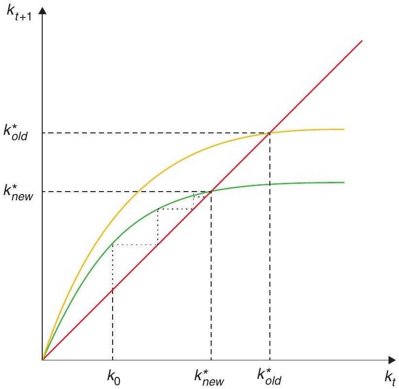
Therefore, the effect of an increase in contributions in a pay-as-you-go system is to shift down the savings locus. The consequences appear in Figure 9.1. The new steady-state capital stock is lower. If the capital stock at the time of the policy shock is to the left of the new steady state, the economy continues to accumulate capital, but at a rate slower than before the change.
9.1.4 Pensions and welfare
Is this a desirable outcome? Does it raise or lower welfare? Suppose before the change \(d_{t}=0\), so the change amounts to introducing pensions in a pay-as-you-go manner. Who is better off as a result?
The old at time \(t\), who now receive total benefits equal to \((1+n) d_{t}\) and contribute nothing, are clearly better off. What about other generations? If \(r\) was less than \(n\) before the introduction of pensions, then the policy change reduces (perhaps totally eliminates) dynamic inefficiency, and all other generations benefit as well. In that case, introducing pensions is Pareto improving. The recent work that we saw in the last chapter suggests that this possibility is not as remote as one may have previously thought. In fact, this idea has coloured some recent policy thinking about reform in places like China.2
But if \(r\) is equal to or larger than \(n\) before the introduction of the pension system, then the policy change creates a conflict. The old at time \(t\) still benefit, but other generations are worse off. In this case, introducing pensions is not Pareto improving. Even if that is the case, this by no means implies that it is always a bad idea politically, or even that is always socially undesirable. The point is that there will be winners and losers, and the relative gains and losses will have to be weighed against one another somehow.
9.2 Moving out of a pay-as-you-go system
The effects on the capital stock from transitioning from a pay-as-you-go system to a fully funded system depend on how the transition is financed. If it is financed with taxes on the young, the capital stock increases. If it is funded by issuing debt, the capital stock may decrease.
There are several transitions associated with the introduction or revamping of pensions systems, and that we may want to analyze. For example, you could move from no pension system and implement a full capitalisation system. As aggregate saving behaviour does not change, we do not expect anything really meaningful to happen from such change in terms of capital accumulation and growth. (That is, of course, to the extent that rational behaviour is a good enough assumption when it comes to individual savings behaviour. We will get back to this pretty soon when we talk about consumption.) Alternatively, as discussed above, if we implement a pay-as-you-go system, the initial old are happy, while the effect for future generations remains indeterminate and depends on the dynamic efficiency of the economy.
However, in recent years it has become fashionable to move away from pay-as-you-go systems to fully funded ones. The reasons for such change is different in each country, but usually can be traced back to deficit and sometimes insolvent systems (sometimes corruption-ridden) that need to be revamped.3 But one of the main reasons was to undo the capital depletion associated with pay-as-you-go systems. Thus, these countries hoped that going for a capitalisation system would increase the capital stock and income over time.
In what remains of this chapter we will show that what happens in such transitions from pay-as-you-go to fully funded systems depends very much on how the transition is financed. There are two options: either the transition is financed by taxing the current young, or it is financed by issuing debt. Both have quite different implications.
To make the analysis simple, in what follows we will keep \(n=0\). (Note that this puts us in the region where \(r>n\), i.e. that of dynamic efficiency.)
Aggregate savings without pensions or with a fully funded system are
\[ s_{t}^{a g g}=\left(\frac{1}{2+\rho}\right) w_{t} . \tag{9.21}\]
With a pay-as-you-go system, they are
\[ s_{t}^{a g g}=s_{t}=\left(\frac{1}{2+\rho}\right) w_{t}-\frac{\left(1+r_{t+1}\right) d+(1+\rho) d}{(2+\rho)\left(1+r_{t+1}\right),} \tag{9.22}\]
which is trivially lower (we knew this already). So now the question is how savings move when going from a pay-as-you-go to a fully funded system. You may think they have to go up, but we need to be careful: we need to take care of the old, who naturally will not be part of the new system, and their retirement income has to be financed. This, in turn, may have effects of its own on capital accumulation.
9.2.1 Financing the transition with taxes on the young
If the transition is financed out of taxes, the young have to use their wages for consumption \(\left(c_{1 t}\right)\), private savings \(\left(s_{t}\right)\), to pay for their contributions ( \(d\) and also for taxes \(\tau_{t}\) ):
\[ c_{1 t}+s_{t}+d+\tau_{t}=w_{t} . \tag{9.23}\]
Future consumption is in turn given by
\[ c_{2 t+1}=\left(1+r_{t+1}\right) s_{t}+\left(1+r_{t+1}\right) d, \tag{9.24}\]
as we are in a fully funded system. Because taxes here are charged to finance the old, we have \(\tau_{t}=d\) (remember we have assumed population growth to be equal to zero). If you follow the logic above, it can be shown that in this case we have
\[ s_{t}^{a g g}=\frac{\left(w_{t}-\tau_{t}\right)}{(2+\rho)} . \tag{9.25}\]
You may notice that this is lower than the steady-state savings rate (next period, i.e. in 30 years, there are no more taxes), but you can also show that it is higher than in the pay-as-you-go system. To do so, replace \(\tau_{t}\) with \(d\) in (9.25) and then compare the resulting expression with that of (9.22).
So savings goes up slowly, approaching its steady-state value. These dynamics are what supports World Bank recommendations that countries should move from pay-as-you-go to fully capitalised systems. Notice however that the reform hurts the current young that have to save for their own and for the current old generation. Then remember that one period here is actually one generation, so it’s something like 30 years. What do you think would be the political incentives, as far as reforming the system, along those lines?
9.2.2 Financing the transition by issuing debt
Now let’s think about how things would change if the transition is financed by issuing debt. (Maybe that is a politically more palatable option!) In this case, for the current young there are no taxes, and debt is another asset that they can purchase:
\[ c_{1 t}+s_{t}+d+g_{\text {debt }}=w_{t}, \tag{9.26}\]
so consumption in old age can be
\[ c_{2 t+1}=\left(1+r_{t+1}\right) s_{t}+\left(1+r_{t+1}\right) d+\left(1+r_{t+1}\right) g_{\text {debt }} . \tag{9.27}\]
Following the same logic as before, private savings are
\[ s_{t}=\frac{w_{t}}{(2+\rho)}-d-g_{d e b t} . \tag{9.28}\]
How about aggregate savings? Note that contributions to the fully funded system \(d\), work as savings from an aggregate perspective: they are available to finance the accumulation of capital. However, the amount of debt issued by the government is in fact not used for capital accumulation, but rather for consumption, because it is a transfer to the old. As such, aggregate savings are given by
\[ s_{t}^{a g g}=s_{t}+d=\frac{w_{t}}{(2+\rho)}-g_{d e b t}=\frac{w_{t}}{(2+\rho)}-d, \tag{9.29}\]
where in the last step we use the fact that (under no population growth) the government issues \(g_{\text {debt }}=d\) of debt to pay benefits to the current old.
Let’s see how this compares to the pay-as-you-go savings. Rewriting equation (9.22) which shows the savings rate in a pay-as-you-go system
\[ s_{t}^{a g g}=s_{t}=\left(\frac{1}{2+\rho}\right) w_{t}-d \frac{\left(1+r_{t+1}\right)+(1+\rho)}{(2+\rho)\left(1+r_{t+1}\right)} . \tag{9.30}\]
Notice that if
\[ \frac{\left(1+r_{t+1}\right)+(1+\rho)}{(2+\rho)\left(1+r_{t+1}\right)}<1, \tag{9.31}\]
then in this case savings is even lower than in the pay-as-you-go system, which happens because the government now pays \(r\) on its debt, which in this case is higher than \(n\).
Another way to see this is if the government imposed a fully funded system but then makes the pension firms purchase government debt that is used for the current old (i.e. for consumption). There is no way this type of reform can increase the capital stock.
9.2.3 Discussion
The above discussion embodies the dimensions of intergenerational equity, the potential efficiency effects, and also the importance of how policies are implemented. Moving from a pay-as-you-go system to a fully funded one is not immune to the way the transition is financed. This should capture your attention: you need to work out fully the effects of policies!
Pension reform has been an important debate in developed and developing countries alike. In the 1990s there was an emerging consensus that moving to a fully funded system would be instrumental in the development of local capital markets. This view triggered reforms in many countries. Here we want to discuss two cases that turned out very different: those of Argentina and Chile.4
Chile, for many years, was considered the poster-child for this reform. It implemented a change to a fully funded system in 1980. Furthermore, this was done at a time of fiscal consolidation. In the framework of the previous section, this is akin to the current working-age generation saving for their own retirement, as well as to pay for their contemporaneous old. As the theory suggested, the resources were deployed into investment, the savings rate, and Chile had a successful growth spurt, which many observers associated with the reform.
Argentina, on the other hand, also migrated to a fully funded system, but rather than streamlining the budget, the deficit increased. In fact, it increased by an amount not very different from the loss in pension funds that were now going to private accounts. In the framework of the previous section, this is akin to financing the transition with debt.
As we saw, in this case the reform reduces savings and, in fact, there was no discernible development of Argentine capital markets. The inflow of contributions into the pension funds went directly to buy government debt. But it was even worse: the bloating of the deficit increased the government’s explicit debt. Of course, the counterpart was a reduction in future pension liabilities. But the market was not persuaded, and in 2001 Argentina plunged into a debt crisis. Many observers associated this macroeconomic crisis to the pension reform. A few years later, Argentina renationalized the pension system, moving away from a fully funded approach. The temptation to do so was big. The current generation basically ate up the accumulated, albeit little, capital stock, again, as predicted in our simple OLG specification.
While the contrast with Chile could not be starker, the system there eventually also came under attack. The math is simple. If the return to investments is 5%, an individual that contributes 10% of her wage to a pension system for say, 42 years, and has an expected pension life of 25 years, can actually obtain a replacement ratio of close to 100% (the exact number is 96%). But reality turned out to be far from that. When looking back at the evidence, the average retirement age in Chile has been around 62 years, and the pension life 25 years. However, people reach retirement with, on average, 20 years of contributions, not 42. This allows for a replacement ratio of only 24%. It is this low replacement ratio that has been the focus of complaints. Thus, most of these attempts eventually introduced some sort of low income protection for the elderly.
9.2.4 Do people save enough?
The above setup assumes that agents optimise their savings to maximise intertemporal utility, with or without pensions. However, there are several reasons why this may not be the case. We will get into more detail in Chapters 11 and 12, but it is worth going over some of the possibilities here, in the context of pensions.
First and foremost, people may believe that if they don’t save, the government will step in and bail them out. If you believe that, why would you save? This time inconsistency feature (the government may tell you to save but, if you don’t, will feel tempted to help you out) may lead to suboptimal savings.
Even in the case of the U.S., where these considerations may not be so relevant, there has been ample discussion about the intensity with which people save for retirement. On the one hand, Scholz et al. (2006) shows that the accumulation of assets of people roughly matches the life cycle hypothesis (which we will see in detail in Chapter 11); on the other hand, there is evidence that suggests that consumption levels drop upon retirement (Bernheim et al. 2001), which is inconsistent with optimal savings. One possible reconciliation of these two facts is given by including the dimension of what type of assets people use for savings. Beshears et al. (2018) show that people save sizable amounts, but they tend to save in illiquid assets. Illiquid assets may provide unusually high returns (for example, owning your house provides steady rental income). Kaplan et al. (2014) estimate that housing services provides an after-tax risk adjusted rate of return of close to 8%. In such a world agents hold a large share of illiquid assets but consumption tracks income while they use some potentially expensive mechanisms to partially smooth consumption.
Present bias has also been mentioned as a reason why people tend to save less than the optimal level. In this case, imposing a pension system that forces people to save may be a ex ante optimal commitment device. We will discuss present bias in detail in Chapter 12.
Finally, recent research on savings for retirement has delivered some interesting new ideas and policy suggestions. One typical way of saving in the U.S. is the 401 K programs, where you save with the benefit of a tax deferral: your income is taxed when withdrawing the funds. These programs are typically arranged with your employer, which matches the contributions with a vesting period to entice labour stability. Yet it has been found that matching is a fairly inefficient way to stimulate savings. Madrian (2013) finds that a matching contribution of 25% increases savings by 5%. In contrast default setting seems, to have a much stronger effect. Madrian and Shea (2001) show that when a company shifted from a default where, unless the worker would opt out, it would start contributing 3% of its salary to a 401K program, they found that fifteen months after the change, 85% of the workers participated, and \(65 \%\) contributed \(3 \%\) of their wages. This compared with only \(49 \%\) participation for those workers hired previously in which only 4% contributed 3%. In short, default standards may be powerful (and cheap) tools for incentivizing savings.
9.3 What have we learned?
In this chapter we applied the standard OLG model to study the issue of social security and pensions. We saw that the implications for capital accumulation can vary dramatically depending on the nature of the system. While fully-funded systems simply offer an alternative mechanisms to private savings, pay-as-you-go systems are essentially intergenerational transfers. These reduce the incentive for private savings, and reduce capital accumulation.
That said, we have also seen that the effects of policy reforms hinge very dramatically on implementation details. For instance, transitioning from pay-as-you-go to a fully funded system can even reduce capital accumulation, if the transition is financed with debt.
Very importantly, the welfare effects of policy interventions are hard to pin down, because there will be winners and losers. Things get even harder if we depart from fully rational behaviour. This also means that the political incentives can be tricky, and they must be taken into consideration.
9.4 What next?
As we anticipated, the OLG framework has become increasingly used in macroeconomics. Many years ago, Auerbach and Kotlikoff (1987) provided an extension of this model to, realistically, allow for 50 generations of working age population. That model became the starting point of a more policy-oriented simulations, which were mostly applied to discussing taxations issues. Azariadis (1993) summarised our knowledge of these models, and is a good starting point for those interested in reviewing standard applications in macroeconomic theory, and understanding the potential of the OLG model to discuss business fluctuations and monetary policy. Ljungqvist and Sargent (2018) provide a more recent update.
But the interesting action has to do with the applications of the OLG model as a workhorse from modern macroeconomics in the age of low interest rates. As we will look into this in later chapters, we defer to the bibliography on this until then.
References
Auerbach, A. J. & Kotlikoff, L. J. (1987). Evaluating fiscal policy with a dynamic simulation model. The American Economic Review, 77(2), 49-55.
Azariadis, C. (1993). Intertemporal macroeconomics.
Bernheim, B. D., Skinner, J., & Weinberg, S. (2001). What accounts for the variation in retirement wealth among U.S. households? American Economic Review, 91(4), 832-857.
Beshears, J., Choi, J. J., Laibson, D., & Madrian, B. C. (2018). Behavioral household finance. Handbook of behavioral economics: Applications and foundations 1 (pp. 177-276). Elsevier.
Feldstein, M. & Bacchetta, P. (1991). National saving and international investment. National saving and economic performance (pp. 201-226). University of Chicago Press.
Kaplan, G., Violante, G. L., & Weidner, J. (2014). The wealthy hand-to-mouth. (tech. rep.). National Bureau of Economic Research.
Ljungqvist, L. & Sargent, T. J. (2018). Recursive macroeconomic theory. MIT Press.
Madrian, B. C. & Shea, D. F. (2001). The power of suggestion: Inertia in 401 (k) participation and savings behavior. The Quarterly Journal of Economics, 116(4), 1149-1187.
Scholz, J. K., Seshadri, A., & Khitatrakun, S. (2006). Are Americans saving “optimally” for retirement? Journal of Political Economy, 114(4), 607-643.
See Feldstein and Bacchetta (1991) for a good non-technical introduction to some of the other issues, including distribution, risk, and labour market implications.↩︎
As an example, check out this headline: ’China hopes social safety net will push its citizens to consume more, save less’ (Washington Post, July 14, 2010).↩︎
Chile is perhaps the best-known example, with its pioneering move in the early 1980s. (See also Feldstein’s discussion.) For a discussion of the real-world pitfalls, Google this NYT article from January 2006: “Chile’s Candidates Agree to Agree on Pension Woes”.↩︎
Maybe because two of us are from Argentina and Chile?↩︎