11 Consumption
The usefulness of the tools that we have studied so far in the book goes well beyond the issue of economic growth and capital accumulation that has kept us busy so far. In fact, those tools enable us to think about all kinds of dynamic issues, in macroeconomics and beyond. As we will see, the same tradeoffs arise again and again: how do individuals trade off today vs tomorrow? It depends on the rate of return, on impatience, and on the willingness to shift consumption over time, all things that are captured by our old friend, the Euler equation! What are the constraints that the market imposes on individual behaviour? You won’t be able to borrow if you are doing something unsustainable. Well, it’s the no-Ponzi game condition! How should we deal with shocks, foreseen and unforeseen? This leads to lending and borrowing and, at an aggregate level, the current account!
All of these issues are raised when we deal with some of the most important (and inherently dynamic) issues in macroeconomics: the determinants of consumption and investment, fiscal policy, and monetary policy. To these issues we will now turn.
We start by looking at one of the most important macroeconomic aggregates, namely consumption. In order to understand consumption, we will go back to the basics of individual optimisation and the intertemporal choice of how much to save and consume. Our investigation into the determinants of consumption will proceed in two steps. First, we will analyse the consumer’s choice in a context of full certainty. We will be careful with the algebra, so readers who feel comfortable with the solutions can skip the detail, while others may find the careful step-by-step procedure useful. Then, in the next chapter, we will add the realistic trait of uncertainty (however simply it is modelled). In the process, we will also see some important connections between macroeconomics and finance.
11.1 Consumption without uncertainty
The main result of the consumption theory without uncertainty is that of consumption smoothing. People try to achieve as smooth a consumption profile as possible, by choosing a consumption level that is consistent with their intertemporal resources and saving and borrowing along the way to smooth the volatility in income paths.
Let’s start with the case where there is one representative consumer living in a closed economy, and no population growth. All quantities (in small-case letters) are per-capita. The typical consumer-worker provides one unit of labour inelastically. Their problem is how much to save and how much to consume
over their lifetime of length \(T\). This (unlike in the analysis of intertemporal choice that we pursued in the context of the Neoclassical Growth Model) will be partial equilibrium analysis: we take the interest rate \(r\) and the wage rate \(w\) as exogenous.
11.1.1 The consumer’s problem
This will be formally very similar to what we have encountered before. The utility function is
\[ \int_{0}^{T} u\left(c_{t}\right) e^{-\rho t} d t \tag{11.1}\]
where \(c_{t}\) denotes consumption and \(\rho(>0)\) is the rate of time preference. Assume \(u^{\prime}\left(c_{t}\right)>0, u^{\prime \prime}\left(c_{t}\right) \leq 0\), and that Inada conditions are satisfied.
The resource constraint is
\[ \dot{b}_{t}=r b_{t}+w_{t}-c_{t}, \tag{11.2}\]
where \(w_{t}\) is the real wage and \(b_{t}\) is the stock of bonds the agent owns. Let us assume that the real interest rate \(r\) is equal to \(\rho\).1
The agent is also constrained by the no-Ponzi game (NPG) or solvency condition:
\[ b_{T} e^{-r T} \geq 0 \tag{11.3}\]
Solution to consumer’s problem
The consumer maximises (11.1) subject to (11.2) and (11.3) for given and \(b_{0}\). The current value Hamiltonian for the problem can be written as
\[ H=u\left(c_{t}\right)+\lambda_{t}\left[r b_{t}+w_{t}-c_{t}\right] . \tag{11.4}\]
Note that \(c\) is a control variable (jumpy), \(b\) is the state variable (sticky), and \(\lambda\) is the costate variable (the multiplier associated with the intertemporal budget constraint, also jumpy). The costate has an intuitive interpretation: the marginal value as of time \(t\) of an additional unit of the state (assets \(b\), in this case).
The optimality conditions are
\[ u^{\prime}\left(c_{t}\right)=\lambda_{t}, \tag{11.5}\]
\[ \frac{\dot{\lambda}_{t}}{\lambda_{t}}=\rho-r, \tag{11.6}\]
\[ \lambda_{T} b_{T} e^{-\rho T}=0 . \tag{11.7}\]
This last expression is the transversality condition (TVC).
11.1.2 Solving for the time profile and level of consumption
Take (11.5) and differentiate both sides with respect to time
\[ u^{\prime \prime}\left(c_{t}\right) \dot{c}_{t}=\dot{\lambda}_{t} . \tag{11.8}\]
Divide this by (11.5) and rearrange
\[ \frac{u^{\prime \prime}\left(c_{t}\right) c_{t}}{u^{\prime}\left(c_{t}\right)} \frac{\dot{c}_{t}}{c_{t}}=\frac{\dot{\lambda}_{t}}{\lambda_{t}} . \tag{11.9}\]
Now, as we’ve seen before, define
\[ \sigma \equiv\left[-\frac{u^{\prime \prime}\left(c_{t}\right) c_{t}}{u^{\prime}\left(c_{t}\right)}\right]^{-1}>0 \tag{11.10}\]
as the elasticity of intertemporal substitution in consumption. Then, (11.9) becomes
\[ \frac{\dot{c}_{t}}{c_{t}}=-\sigma \frac{\dot{\lambda}_{t}}{\lambda_{t}} . \tag{11.11}\]
Finally using (11.6) in (11.11) we obtain (what a surprise!):
\[ \frac{\dot{c}_{t}}{c_{t}}=\sigma(r-\rho)=0 . \tag{11.12}\]
Equation (11.12) says that consumption is constant since we assume \(r=\rho\). It follows then that
\[ c_{t}=c^{*}, \tag{11.13}\]
so that consumption is constant.
We now need to solve for the level of consumption \(c^{*}\). Using (11.13) in (11.2) we get
\[ \dot{b}_{t}=r b_{t}+w_{t}-c^{*}, \tag{11.14}\]
which is a differential equation in \(b\), whose solution is, for any time \(t>0\),
\[ b_{t}=\int_{0}^{t} w_{s} e^{r(t-s)} d s-\left(e^{r t}-1\right) \frac{c^{*}}{r}+b_{0} e^{r t} . \tag{11.15}\]
where time \(v\) is any moment between 0 and \(t\). Evaluating this at \(t=T\) (the terminal period) we obtain the stock of bonds at the end of the agent’s life:
\[ b_{T}=\int_{0}^{T} w_{s} e^{r(T-s)} d s-\left(e^{r T}-1\right) \frac{c^{*}}{r}+b_{0} e^{r T} \tag{11.16}\]
Dividing both sides by \(e^{r T}\) and rearranging, we have
\[ b_{T} e^{-r T}=\int_{0}^{T} w_{t} e^{-r s} d s-\left(1-e^{-r T}\right) \frac{c^{*}}{r}+b_{0} \tag{11.17}\]
Notice that using (11.5), (11.7), and (11.13), the TVC can be written as
\[ u^{\prime}\left(c^{*}\right) b_{T} e^{-r T}=0 . \tag{11.18}\]
Since clearly \(u^{\prime}\left(c^{*}\right) \neq 0\) (this would require \(c^{*} \rightarrow \infty\) ), for the TVC to hold it must be the case that \(b_{T} e^{-r T}=0\). Applying this to (11.17) and rearranging we have
\[ \frac{c^{*}}{r}\left(1-e^{-r T}\right)=b_{0}+\int_{0}^{T} w_{s} e^{-r s} d s \tag{11.19}\]
The LHS of this equation is the net present value (NPV) of consumption as of time 0, and the RHS the NPV of resources as of time 0.
11.2 The permanent income hypothesis
Dividing (11.19) through by \(\left(1-e^{-r T}\right)\) and multiplying through by \(r\) we have
\[ c^{*}=\frac{r b_{0}+r \int_{0}^{T} w_{t} e^{-r t} d t}{1-e^{-r T}} . \tag{11.20}\]
The RHS of this expression can be thought of as the permanent income of the agent as of time 0. That is what they optimally consume.
What is savings in this case? Define
\[ \begin{aligned} s_{t} & =w_{t}+r b_{t}-c_{t} \\ & =r\left(b_{t}-\frac{b_{0}}{1-e^{-r T}}\right)+\left(w_{t}-\frac{r \int_{0}^{T} w_{t} e^{-r t} d t}{1-e^{-r T}}\right) \end{aligned} \tag{11.21}\]
Hence, savings is high when a) bond-holdings are high relative to their permanent level, and b) current wage income is high relative to its permanent level. Conversely, when current income is less than permanent income, saving can be negative. Thus, the individual uses saving and borrowing to smooth the path of consumption. (Where have we seen that before?)
This is the key idea of Friedman (1957). Before then, economists used to think of a rule of thumb in which consumption would be a linear function of current disposable income. But if you think about it, from introspection, is this really the case? It turns out that the data also belied that vision, and Friedman (1957) gave an explanation for that.
11.2.1 The case of constant labour income
Note also that if \(w_{t}=w\), the expression for consumption becomes
\[ c^{*}=\frac{r b_{0}+r w \int_{0}^{T} e^{-r t} d t}{1-e^{-r T}}=\frac{r b_{0}}{1-e^{-r T}}+w . \tag{11.22}\]
Moreover, if \(T \rightarrow \infty\), this becomes
\[ c^{*}=r b_{0}+w, \tag{11.23}\]
which has a clear interpretation: \(r b_{0}+w\) is what the agent can consume on a permanent (constant) basis forever.
What is the path of bond-holdings over time? Continue considering the case in which \(w\) is constant, but \(T\) remains finite. In that case the equation for bonds (11.15) becomes
\[ b_{t}=\left(e^{r t}-1\right) \frac{w-c^{*}}{r}+b_{0} e^{r t} . \tag{11.24}\]
Using (11.22) in here we get
\[ b_{t}=\left(\frac{1-e^{-r(T-t)}}{1-e^{-r T}}\right) b_{0}<b_{0} . \tag{11.25}\]
Notice that
\[ \frac{d b_{t}}{d t}=-r\left(\frac{e^{-r(T-t)}}{1-e^{-r T}}\right) b_{0}<0 \tag{11.26}\]
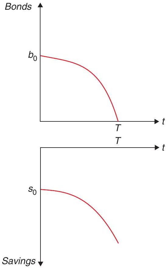
\[ \frac{d^{2} b_{t}}{d t^{2}}=-r^{2}\left(\frac{e^{-r(T-t)}}{1-e^{-r T}}\right) b_{0}<0, \tag{11.27}\]
so that bond-holdings decline, and at an accelerating rate, until they are exhausted at time \(T\). Figure 11.1 shows this path.
11.2.2 The effects of non-constant labour income
Suppose now that wages have the following path:
\[ w_{t}=\left\{\begin{array}{l} w^{H}, 0 \leq t<T^{\prime} \\ w^{L}, T^{\prime} \leq t<T \end{array}, T^{\prime}<T, w^{H}>w^{L} .\right. \tag{11.28}\]
Then, we can use (11.20) to figure out what constant consumption is:
\[ c^{*} =\frac{r b_{0}+w^{H} r \int_{0}^{T^{\prime}} e^{-r t} d t+w^{L} r \int_{T^{\prime}}^{T} e^{-r t} d t}{1-e^{-r T}} \tag{11.29}\]
\[ =\frac{r b_{0}+w^{H}\left(1-e^{-r T^{\prime}}\right)+w^{L}\left(e^{-r T^{\prime}}-e^{-r T}\right)}{1-e^{-r T}} . \tag{11.30}\]
For \(t<T^{\prime}\), saving is given by
\[ \begin{aligned} s_{t} & =w^{H}+r b_{t}-c_{t}\\ & =r\left(b_{t}-\frac{b_{0}}{1-e^{-r T}}\right)+\left(w^{H}-\frac{w^{H}\left(1-e^{-r T^{\prime}}\right)+w^{L}\left(e^{-r T^{\prime}}-e^{-r T}\right)}{1-e^{-r T}}\right) \end{aligned} \tag{11.31}\]
What are bond-holdings along this path? In this case the equation for bonds (11.15) becomes, for \(t<T^{\prime}\)
\[ b_{t}=b_{0} \frac{1-e^{-r(T-t)}}{1-e^{-r T}}+\left(e^{r t}-1\right) \frac{w^{H}-w^{L}}{r}\left(\frac{e^{-r T^{\prime}}-e^{-r T}}{1-e^{-r T}}\right) . \tag{11.32}\]
Notice
\[ \frac{d b_{t}}{d t}=\left\{-r b_{0} \frac{e^{-r T}}{1-e^{-r T}}+\left(w^{H}-w^{L}\right)\left(\frac{e^{-r T^{\prime}}-e^{-r T}}{1-e^{-r T}}\right)\right\} e^{r t} \tag{11.33}\]
\[ \frac{d^{2} b_{t}}{d t^{2}}=\left\{-r b_{0} \frac{e^{-r T}}{1-e^{-r T}}+\left(w^{H}-w^{L}\right)\left(\frac{e^{-r T^{\prime}}-e^{-r T}}{1-e^{-r T}}\right)\right\} r e^{r t} \tag{11.34}\]
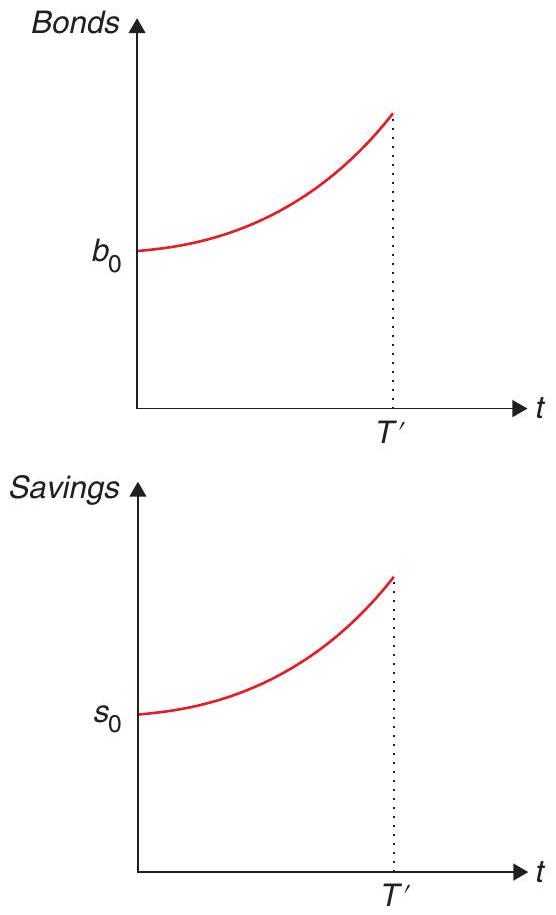
so that bond-holdings are increasing at an increasing rate for \(t<T^{\prime}\) if \(b_{0}\) is sufficiently small.
Plugging this into (11.31) we obtain
\[ \begin{aligned} s_{t}= & -\left(\frac{e^{-r(T-t)}}{1-e^{-r T}}\right) r b_{0}+w^{H} \\ & -w^{H}\left[1-e^{r t}\left(\frac{e^{-r T^{\prime}}-e^{-r T}}{1-e^{-r T}}\right)\right]-w^{L} e^{r t}\left(\frac{e^{-r T^{\prime}}-e^{-r T}}{1-e^{-r T}}\right) \end{aligned} \]
so that, yet again savings is high when current wage income is above permanent wage income.
Simplifying, this last expression becomes
\[ s_{t}=\left\{-r b_{0} \frac{e^{-r T}}{1-e^{-r T}}+\left(w^{H}-w^{L}\right)\left(\frac{e^{-r T^{\prime}}-e^{-r T}}{1-e^{-r T}}\right)\right\} e^{r t} . \tag{11.35}\]
Notice
\[ \frac{d s_{t}}{d t}=\left\{-r b_{0} \frac{e^{-r T}}{1-e^{-r T}}+\left(w^{H}-w^{L}\right)\left(\frac{e^{-r T^{\prime}}-e^{-r T}}{1-e^{-r T}}\right)\right\} r e^{r t} \tag{11.36}\]
\[ \frac{d^{2} s_{t}}{d t^{2}}=\left\{-r b_{0} \frac{e^{-r T}}{1-e^{-r T}}+\left(w^{H}-w^{L}\right)\left(\frac{e^{-r T^{\prime}}-e^{-r T}}{1-e^{-r T}}\right)\right\} r^{2} e^{r t} \tag{11.37}\]
so that, if \(b_{0}\) is sufficiently small, bond-holdings rise, and at an accelerating rate, until time \(T^{\prime}\). Figure11.2 shows this path. This is consumption smoothing: since the current wage is higher than the future wage, the agent optimally accumulates assets.
11.3 The life-cycle hypothesis
The most notable application of the model with non-constant labour income is that of consumption over the life cycle. Assume \(b_{0}=0\), and also that income follows
\[ w_{t}=\left\{\begin{array}{l} w>0,0 \leq t<T^{\prime} \\ 0, T^{\prime} \leq t<T \end{array}, T^{\prime}<T\right. \]
so that now the worker-consumer works for the first \(T^{\prime}\) periods of his life, and is retired for the remaining \(T-T^{\prime}\) periods.
Then, consumption is simply given by (11.29) with \(b_{0}=0, w^{H}=w, w^{L}=0\) :
\[ c^{*}=w\left(\frac{1-e^{-r T^{\prime}}}{1-e^{-r T}}\right)<w \tag{11.38}\]
so that consumption per instant is less than the wage.
Let us now figure out what bond-holdings are during working years \(\left(t \leq T^{\prime}\right)\). Looking at (11.32), and using (11.38), we can see that
\[ \begin{aligned} & b_{t}=\int_{0}^{t} w e^{r(t-s)} d s-\left(e^{r t}-1\right) \frac{w}{r}\left(\frac{1-e^{-r T^{\prime}}}{1-e^{-r T}}\right) \Rightarrow \\ & b_{t}=\frac{w e^{r t}}{r}\left[1-e^{-r t}\right]-\left(e^{r t}-1\right) \frac{w}{r}\left(\frac{1-e^{-r T^{\prime}}}{1-e^{-r T}}\right) \Rightarrow \\ & b_{t}=\frac{w}{r}\left[e^{r t}-1\right]-\left(e^{r t}-1\right) \frac{w}{r}\left(\frac{1-e^{-r T^{\prime}}}{1-e^{-r T}}\right) \Rightarrow \\ & b_{t}=\frac{w}{r}\left[e^{r t}-1\right]\left[\frac{\left(1-e^{-r T}\right)-\left(1-e^{r T^{\prime}}\right)}{1-e^{-r T}}\right] \Rightarrow \\ & b_{t}=\frac{w}{r}\left(e^{r t}-1\right)\left(\frac{e^{-r T^{\prime}}-e^{-r T}}{1-e^{-r T}}\right) . \end{aligned} \tag{11.39}\]
By the same token, savings during the working years \(\left(t \leq T^{\prime}\right)\) can be obtained simply by differentiating this expression with respect to time:
\[ s_{t} \equiv \frac{d b_{t}}{d t}=w e^{r t}\left(\frac{e^{-r T^{\prime}}-e^{-r T}}{1-e^{-r T}}\right) \tag{11.40}\]
so that
\[ \frac{d s_{t}}{d t} \equiv \frac{d^{2} b_{t}}{d t^{2}}=r w e^{r t}\left(\frac{e^{-r T^{\prime}}-e^{-r T}}{1-e^{-r T}}\right)>0 \tag{11.41}\]
\[ \frac{d^{2} s_{t}}{d t^{2}}=r^{2} w e^{r t}\left(\frac{e^{r T^{\prime}}-e^{-r T}}{1-e^{-r T}}\right)>0 \tag{11.42}\]
What happens after the time of retirement \(T^{\prime}\) ? To calculate bond-holdings, notice that for \(t \geq T^{\prime}\), (11.25) gives
\[ b_{t}=\frac{w}{r}\left(1-e^{r(t-T)}\right)\left(\frac{1-e^{-r T^{\prime}}}{1-e^{-r T}}\right) \tag{11.43}\]
so that
\[ s_{t} \equiv \frac{d b_{t}}{d t}=-w e^{r(t-T)}\left(\frac{1-e^{-r T^{\prime}}}{1-e^{-r T}}\right)<0 \tag{11.44}\]
\[ \frac{d s_{t}}{d t} \equiv \frac{d^{2} b_{t}}{d t^{2}}=-r w e^{r(t-T)}\left(\frac{1-e^{-r T^{\prime}}}{1-e^{-r T}}\right)<0 \tag{11.45}\]
\[ \frac{d^{2} s_{t}}{d t^{2}}=-r^{2} w e^{r(t-T)}\left(\frac{1-e^{-r T^{\prime}}}{1-e^{-r T}}\right)<0 \tag{11.46}\]
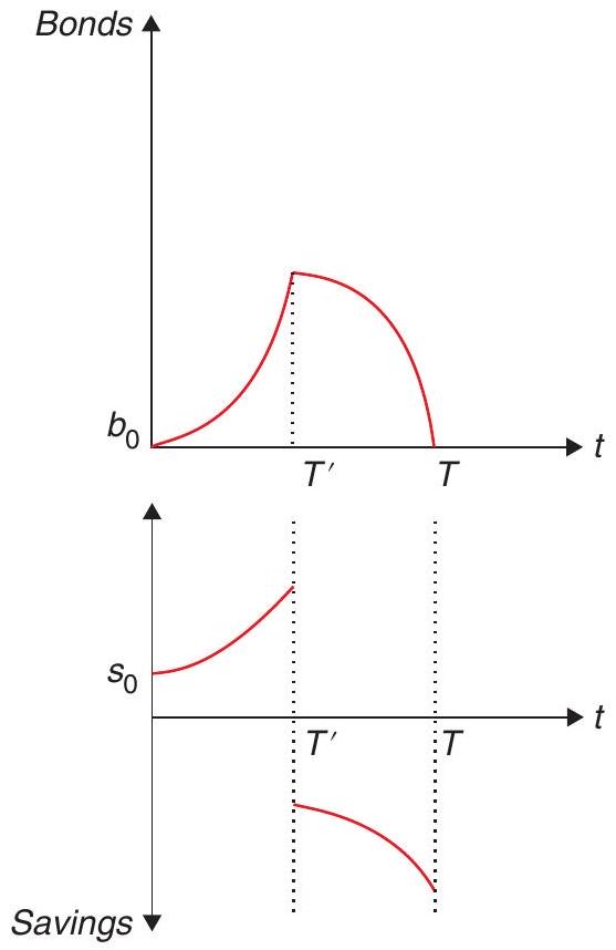
so that savings decrease over time.
Figure 11.3 shows this path. The agent optimally accumulates assets until retirement time \(T^{\prime}\), then depletes them between time \(T^{\prime}\) and time of death \(T\). This is the basic finding of the life-cycle hypothesis of Modigliani and Brumberg (1954).2
Of course, the life-cycle hypothesis is quite intuitive. One way or the other we all plan for retirement (or trust the government will). Scholz et al. (2006) show that \(80 \%\) of the households over age 50 had accumulated at least as much wealth as a life-cycle model prescribes, and the the wealth deficit of the remaining 20% is relatively small, thus providing support for the model. On the other hand, many studies have also found that consumption falls at retirement. For example, Bernheim et al. (2001) show that there is a drop in consumption at retirement and that it is larger with families with a lower replacement rates from Social Security and pension benefits. This prediction is at odds with the life-cycle hypothesis.
References
Bernheim, B. D., Skinner, J., & Weinberg, S. (2001). What accounts for the variation in retirement wealth among U.S. households? American Economic Review, 91(4), 832-857.
Friedman, M. (1957). The permanent income hypothesis. A theory of the consumption function (pp. 20-37). Princeton University Press.
Modigliani, F. & Brumberg, R. (1954). Utility analysis and the consumption function: An interpretation of cross-section data. Franco Modigliani, 1(1), 388-436.
Scholz, J. K., Seshadri, A., & Khitatrakun, S. (2006). Are Americans saving “optimally” for retirement? Journal of Political Economy, 114(4), 607-643.
Do you remember our discussion of the open-economy Ramsey model, and the implications of \(r>\rho\) or \(r<\rho\) ?↩︎
What explains the curvature? In other words, why is it that the individual accumulates at a faster rate as she approaches retirement, and then decumulates at a faster rate as she approaches death? The intuition is that, because of her asset accumulation, the individual’s interest income increases as she approaches retirement - for a constant level of consumption, that means she saves more and accumulates faster. the flip-side of this argument happens close to the death threshold, as interest income gets lower and dissaving intensifies as a result.↩︎