19 Monetary policy: An introduction
19.1 The conundrum of money
We have finally reached our last topic: monetary policy (MP), one of the most important topics in macroeconomic policy, and perhaps the most effective tool of macroeconomic management. While among practitioners there is a great deal of consensus over the way monetary policy should be implemented, it always remains a topic where new ideas flourish and raise heated debates. Paul Krugman tweeted,
Nothing gets people angrier than monetary theory. Say that Trump is a traitor and they yawn; say that fiat money works and they scream incoherently.
Our goal in these final chapters is to try to sketch the consensus, its shortcomings, and the ongoing attempts to rethink MP for the future, even if people scream!
We will tackle our analysis of monetary policy in three steps. In this chapter we will start with the basics: the relation of money and prices, and the optimal choice of inflation. This will be developed first, in a context where output is exogenous. This simplifies relative to the New Keynesian approach we discussed in Chapter 15, but will provide some of the basic intuitions of monetary policy. The interaction of money and output creates a whole new wealth of issues. Is monetary policy inconsistent? Should it be conducted through rules or with discretion? Why is inflation targeting so popular among central banks? We will discuss these questions in the next chapter. Finally, in the last two chapters we will discuss new frontiers in monetary policy, with new challenges that have become more evident in the new period of very low interest rates. In Chapter 21 we discuss monetary policy when constrained by the lower bound, and the new approach of quantitative easing. In Chapter 22 we discuss a series of topics: secular stagnation, the fiscal theory of the price level, and bubbles. Because these last two chapters are more prolific in referencing this recent work, we do not add the what next section at the end of the chapter, as the references for future exploration are already plenty within the text.
But before we jump on to this task, let us briefly note that monetary economics rests on a fairly shaky foundation: the role of money - why people hold it, and what are its effects on the economy - is one of the most important issues in macroeconomics, and yet it is one of the least understood. Why is this? For starters, in typical micro models - and pretty much in all of our macro models as well - we did not deal with money: the relevant issues were always discussed in terms of relative prices,
not nominal prices. There was no obvious (or, at least, essential) role for money in the NGM that we used throughout this book. In fact, the non plus ultra of micro models, the general equilibrium Arrow-Debreu framework, not only does not need money, it also does not have trading! (Talk about outrageous assumptions.) In that model, all trades are consummated at the beginning of time, and then you have the realisation of these trades, but no new trading going on over time. Of course, the world is not that complete, so we need to update our trading all the time. We use money as an insurance for these new trades. However, it is much easier to say people use money for transactions than to model it, because we need to step into the world of incomplete markets, and we do not know how to handle that universe well.
The literature has thus taken different paths for introducing money into general equilibrium models. The first is to build a demand for money from micro-foundations. The question here is whether one commodity (maybe gold, shells, salt?) may become a vehicle that people may naturally choose for transactions, i.e. what we usually refer to as money. Kiyotaki and Wright (1989), for example, go this way. While nice, by starting from first principles, this approach is intractable and did not deliver models which are sufficiently flexible to discuss other issues, so this research has only produced a plausible story for the existence of money but not a workable model for monetary policy.
The other alternative is to introduce money in our typical overlapping generations model. Money serves the role of social security, and captures the attractive feature that money has value because you believe someone down the road will take it. Unfortunately, the model is not robust. Any asset that dominates money in rate of return will simply crowd money out of the system, thus making it impossible to use this model to justify the use of money in cases in which the inflation rate is minimally positive when money is clearly dominated in rate of return.
A third approach is to just assume that money needs to be used for purchases, the so-called cash in advance constraints. In this framework the consumer splits itself at the beginning of each period into a consumer self and a producer self. Given that the consumer does not interact with the producer, she needs to bring cash from the previous period, thus the denomination of cash in advance. This is quite tractable, but has the drawback that gives a very rigid money demand function (in fact, money demand is simply equal to consumption).
A more flexible version is to think that the consumer has to devote some time to shopping, and that shopping time is reduced by the holdings of money. This provides more flexibility about thinking in the demand for money.
Finally, a take-it-all-in alternative is just to add money in the utility function. While this is a reduced form, it provides a flexible money demand framework, and, therefore, has been used extensively in the literature. At any rate, it is obvious that people demand money, so we just postulate that it provides utility. An additional benefit is that it can easily be accommodated into the basic framework we have been using in this book, for example, by tacking it to an optimisation problem akin to that of the NGM.
Thus, we will go this way in this chapter. As you will see, it provides good insights into the workings of money in the economy.
19.1.1 Introducing money into the model
Let’s start with the simplest possible model. Output exogenous, and a government that prints money and rebates the proceeds to the consumer. We will lift many of these assumptions as we go along. But before we start we need to discuss the budget constraints.
Assume there is only one good the price of which in terms of money is given by \(P_{t}\). The agent can hold one of two assets: money, whose nominal stock is \(M_{t}\), and a real bond, whose real value is given, as in previous chapters, by \(b_{t}\). Note that we now adopt the convention that real variables take on small-case letters, and nominal variables are denoted by capital letters. The representative agent’s budget constraint is given by
\[ \frac{\dot{M}_{t}}{P_{t}}+\dot{b}_{t}=r b_{t}+y_{t}-\tau_{t}-c_{t}, \tag{19.1}\]
where \(\tau_{t}\) is real taxes paid to the government and, as usual, \(y_{t}\) is income and \(c_{t}\) consumption. Define the real quantity of money as
\[ m_{t}=\frac{M_{t}}{P_{t}} . \tag{19.2}\]
Taking logs of both sides, and then time derivatives, we arrive at:
\[ \dot{m}_{t}=m_{t} \frac{\dot{M}_{t}}{M_{t}}-m_{t} \frac{\dot{P}_{t}}{P_{t}}=\frac{M_{t}}{P_{t}} \frac{\dot{M}_{t}}{M_{t}}-m_{t} \frac{\dot{P}_{t}}{P_{t}} . \tag{19.3}\]
Defining \(\pi_{t} \equiv \frac{\dot{P}_{t}}{P_{t}}\) as the rate of inflation and rearranging, we have:
\[ \frac{\dot{M}_{t}}{P_{t}}=\dot{m}_{t}+\pi_{t} m_{t} . \tag{19.4}\]
The LHS of (19.4) is the real value of the money the government injects into the system. We call this total revenue from money creation, or seigniorage. Notice from the RHS of (19.4) that this has two components:
The term \(\dot{m}_{t}\) is the increase in real money holdings by the public. (It is sometimes referred to as seigniorage as well; we’ll keep our use consistent).
The term \(m_{t} \pi_{t}\) is the inflation tax: the erosion, because of inflation, of the real value of the money balances held by the public. We can think of \(m_{t}\) as the tax base, and \(\pi_{t}\) as the tax rate.
Using (19.4) in (19.1) we have that
\[ \dot{m}_{t}+\dot{b}_{t}=r b_{t}+y_{t}-\tau_{t}-c_{t}-\pi_{t} m_{t} . \tag{19.5}\]
On the LHS we have accumulation by the agent of the two available financial assets: money and bonds. The last term on the RHS is an additional expense: taxes paid on the real balances held.
Let us consider a steady state in which all variables are constant, then (19.5) becomes
\[ r b+y=\tau+c+\pi m . \tag{19.6}\]
Hence, total income on the LHS must be enough to finance total expenditures (including regular taxes \(\tau\) and the inflation \(\operatorname{tax} \pi m\) ).
A useful transformation involves adding and subtracting the term \(r m_{t}\) to the RHS of (19.5):
\[ \dot{m}_{t}+\dot{b}_{t}=r\left(m_{t}+b_{t}\right)+y_{t}-\tau_{t}-c_{t}-\left(r+\pi_{t}\right) m_{t} . \tag{19.7}\]
Now define
\[ a_{t}=m_{t}+b_{t} \tag{19.8}\]
as total financial assets held by the agent, and
\[ i_{t}=r+\pi_{t} \tag{19.9}\]
as the nominal rate of interest. Using these two relationships in (19.7) we get
\[ \dot{a}_{t}=r a_{t}+y_{t}-\tau_{t}-c_{t}-i_{t} m_{t} . \tag{19.10}\]
The last term on the RHS shows that the cost of holding money, in an inflationary environment, is the nominal rate of interest \(i_{t}\).
19.2 The Sidrauski model
Following Sidrauski (1967), we assume now the representative agent’s utility function is
\[ \int_{0}^{\infty}\left[u\left(c_{t}\right)+v\left(m_{t}\right)\right] e^{-\rho t} d t . \tag{19.11}\]
Here \(v\left(m_{t}\right)\) is utility from holdings of real money balances. Assume \(v^{\prime}\left(m_{t}\right) \geq 0, v^{\prime \prime}\left(m_{t}\right)<0\) and that Inada conditions hold. The agent maximises (19.11) subject to (19.10), which we repeat here for clarity, though assuming, without loss of generality, that output remains constant
\[ \dot{a}=r a_{t}+y-\tau_{t}-c_{t}-i_{t} m_{t}, \]
plus the standard solvency condition
\[ \lim _{T \rightarrow \infty}\left[a_{T} e^{-r T}\right] \geq 0, \tag{19.12}\]
and the initial condition \(a_{0}\). The Hamiltonian is
\[ H=\left[u\left(c_{t}\right)+v\left(m_{t}\right)\right]+\lambda_{t}\left(r a_{t}+y-\tau_{t}-c_{t}-i_{t} m_{t}\right), \tag{19.13}\]
where \(m_{t}\) and \(c_{t}\) are control variables, \(a_{t}\) is the state variable and \(\lambda_{t}\) is the co-state. First order conditions for a maximum are
\[ u^{\prime}\left(c_{t}\right)=\lambda_{t}, \tag{19.14}\]
\[ v^{\prime}\left(m_{t}\right)=\lambda_{t} i_{t}, \tag{19.15}\]
\[ \dot{\lambda}_{t}=\lambda_{t}(\rho-r)=0, \tag{19.16}\]
where the last equality comes from assuming \(r=\rho\) as usual. Equations (19.14) and (19.16) together imply that \(c_{t}\) is constant and equal to \(c\) for all \(t\). Using this fact and combining (19.14) and (19.15) we have
\[ v^{\prime}\left(m_{t}\right)=i_{t} u^{\prime}(c) . \tag{19.17}\]
We can think of equation (19.17) as defining money demand: demand for real balances is decreasing in the nominal interest rate \(i_{t}\) and increasing in steady state consumption \(c\). This is a way to microfound the traditional money demand functions you all have seen before, where demand would be a positive function of income (because of transactions) and a negative function of the nominal interest rate, which is the opportunity cost of holding money.
19.2.1 Finding the rate of inflation
What would the rate of inflation be in this model? In order to close the model, notice that
\[ \frac{\dot{m}_{t}}{m_{t}}=\sigma-\pi_{t}, \tag{19.18}\]
where \(\sigma\) is the rate of money growth. We will also assume that the money printing proceeds are rebated to the consumer, which means that
\[ \tau=-\sigma m . \tag{19.19}\]
Replacing (19.18) and (19.19) into (19.10), using \(\rho=r\), and realizing the agent has no incentive to hold debt, gives that \(c=y\), so that marginal utility is also constant and can be normalised to 1 . Using (19.9), equation (19.17) becomes
\[ v^{\prime}\left(m_{t}\right)=\rho+\pi_{t}, \tag{19.20}\]
which substituting in (19.18) gives
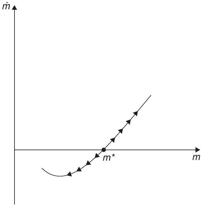
\[ \dot{m}_{t}=(\rho+\sigma) m_{t}-v^{\prime}\left(m_{t}\right) m_{t} . \tag{19.21}\]
Equation (19.21) is a differential equation that defines the equilibrium. Notice that because \(v^{\prime \prime}(m)<0\), this is an unstable differential equation. As the initial price level determines the initial point ( \(m\) is a jump variable in our definitions of Chapter 3), the equilibrium is unique at the point where \(\dot{m}_{t}=0\). The dynamics are shown in Figure 19.1.
This simple model provides some of the basic intuitions of monetary theory.
- An increase in the quantity of nominal money will leave \(m\) unchanged and just lead to a jump in the price level. This is the quantitative theory of money that states that any increase in the stock of money will just result in an equivalent increase in prices.
The rate of inflation is the rate of growth of money (see equation (19.18)). Inflation is a monetary phenomenon.
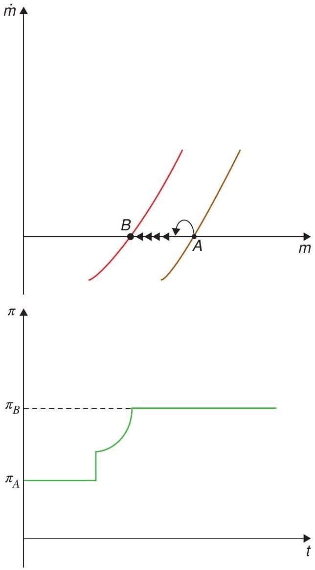
What happens if, suddenly, the rate of growth of money is expected to grow in the future? The dynamics entail a jump in the price level today and a divergent path which places the economy at its new equilibrium when the rate of growth finally increases. In short, increases in future money affect the price and inflation levels today. The evolution of \(m\) and \(\pi\) are shown in Figure 19.2.
Does the introduction of money affect the equilibrium? It doesn’t. Consumption is equal to income in all states of nature. This result is called the neutrality of money.
19.2.2 The optimal rate of inflation
Let’s assume now that we ask a central planner to choose the inflation rate in order to maximise welfare. What \(\sigma\), and, therefore, what inflation rate would be chosen?
We know from (19.20) and (19.17) that the steady-state stock of money held by individuals solves the equation
\[ v^{\prime}(m)=(\rho+\pi)=(\rho+\sigma) . \tag{19.22}\]
This means that the central bank can choose \(\sigma\) to maximise utility from money-holdings. This implies choosing
\[ \pi^{\text {best }}=\sigma^{\text {best }}=-\rho<0, \tag{19.23}\]
so that
\[ v^{\prime}\left(m^{\text {best }}\right)=0 . \tag{19.24}\]
This means that \(m^{\text {best }}\) is the satiation stock of real balances and you achieve it by choosing a negative inflation rate. This is the famous Friedman rule for optimal monetary policy. What’s the intuition? You should equate the marginal cost of holding money from an individual perspective (the nominal interest rate) to the social cost of printing money, which is essentially zero. A zero nominal rate implies an inflation rate that is equal to minus the real interest rate.
In practice, we don’t see a lot of central banks implementing deflationary policy. Why is it so? Probably because deflation has a lot of costs that are left out of this model: its effect on debtors, on aggregate demand, etc., likely in the case when prices and wages tend to be sticky downwards.
We should thus interpret our result as meaning that policy makers should aim for low levels of inflation, so as to keep social and private costs close. In any case, there is a huge literature on the costs of inflation that strengthens the message of this result, we will come back to this at the end of the chapter.
19.2.3 Multiple equilibria in the Sidrauski model
In the previous section we analysed the steady state of the model, but, in general, we have always been cautious as to check if other equilibria are possible. In this monetary model, as it happens, they are.
Figure 19.3 shows the possible configurations for equation (19.21), for all \(m\). We know that
\[ \left.\frac{\partial \dot{m}}{\partial m}\right|_{S S}=-v^{\prime \prime}(m)>0, \tag{19.25}\]
so that the curve crosses the steady state with a positive slope. But what happens to the left of the steady state? Figure 19.3, shows two paths depending on whether the value of the term \(v^{\prime}(m) m\) approaches zero or a positive number as \(m\) approaches zero. If money is very essential and its marginal utility is very high as you reduce your holdings of money, then \(v^{\prime}(m) m>0\) as \(m\) approaches zero. This case corresponds to the path denoted by the letter B. If \(v^{\prime}(m) m \rightarrow 0\), as \(m \rightarrow 0\) then the configuration is of the path leading to A.
With this we can now study other equilibria. The paths to the right are deflationary paths, where inflation is negative and real balances increase without bound. We do not see these increasing deflationary paths, so, from an empirical point of view, they do not seem very relevant (mathematically they are feasible, and some people resorted to these equilibria to explain the low inflation rates in the U.S. in recent years, see Sims (2016)). The paths to the left of the steady state are inflationary paths. Paths along the B curve are inconsistent, as they require \(\dot{m}<0\) when \(m\) hits zero, which is unfeasible. However, paths that do end up at zero, denoted A in Figure 19.3, are feasible. In these cases money is not so essential, so it is wiped out by a hiperinflationary process. In a classical paper, Cagan (1956)
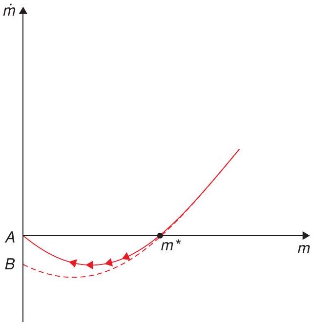
speculated on the possibility of these self-sustaining inflationary dynamics in which the expectation of higher inflation leads to lower money demand, fuelling even higher inflation. So these feasible paths to the left of the steady state could be called Cagan equilibria. The general equilibrium version of the Cagan equilibria described here was first introduced by Obstfeld and Rogoff (1983).
19.2.4 Currency substitution
The model is amenable to discussing the role of currency substitution, that is, the possibility of phasing out the currency and being replaced by a sounder alternative.
The issue of understanding how different currencies interact, has a long tradition in monetary economics. Not only because, in antiquity, many objects operated as monies, but also because, prior to the emergence of the Fed, currency in the U.S. were issued by commercial banks, so there was an innumerable number of currencies circulating at each time. A popular way to think this issue is Gresham’s Law; faced with a low quality currency and a high quality currency, Gresham’s Law argues that people will try to get rid of the low quality currency while hoarding the high quality currency, bad money displaces good money. Of course while this may be true at the individual level, it may not be so at the aggregate level because prices may increase faster when denominated in units of the bad-quality currency debasing its value. Sturzenegger (1994) discusses this issue and makes two points.
When there are two or more currencies, it is more likely that the condition \(v^{\prime}(m) m=0\) is satisfied (particularly for the low quality currency). Thus, the hyperinflation paths are more likely.
If the dynamics of money continue are described by an analogous to (19.21) such as
\[ \dot{m}_{1}=\left(\rho+\sigma_{1}\right) m_{1}-v^{\prime}\left(m_{1}, m_{2}\right) m_{1}, \tag{19.26}\]
notice that if the second currency \(m_{2}\) reduces the marginal utility of the first one, then the inflation rate on the equilibrium path is lower: less inflation is needed to wipe out the currency.
This pattern seems to have occurred in a series of hyperinflations in Argentina in the late 80s, each new wave coming faster but with lower inflation. Similarly, at the end of the 2000s, also in Argentina, very tight monetary conditions during the fixed exchange regime led to the development of multiple private currencies. Once the exchange rate regime was removed, these currencies suffered hyperinflations and disappeared in a wink (see Colacelli and Blackburn 2009).
19.2.5 Superneutrality
How do these results extend to a model with capital accumulation? We can see this easily also in the context of the Sidrauski model (we assume no population growth), but where we give away the assumption of exogenous output and allow for capital accumulation. Consider now the utility function
\[ \int_{0}^{\infty} u\left(c_{t}, m_{t}\right) e^{-\rho t} d t \tag{19.27}\]
where \(u_{c}, u_{m}>0\) and \(u_{c c}, u_{m m}<0\). However, we’ll allow the consumer to accumulate capital now. Defining again \(a=k+m\), the resource constraint can be written as
\[ \dot{a}_{t}=r_{t} a_{t}+w_{t}-\tau_{t}-c_{t}-i_{t} m_{t} . \tag{19.28}\]
The Hamiltonian is
\[ H=u\left(c_{t}, m_{t}\right)+\lambda_{t}\left[r a_{t}+w_{t}-\tau_{t}-c_{t}-i_{t} m_{t}\right] . \tag{19.29}\]
The FOC are, as usual,
\[ u_{c}\left(c_{t}, m_{t}\right)=\lambda_{t}, \tag{19.30}\]
\[ u_{m}\left(c_{t}, m_{t}\right)=\lambda_{t} i_{t}, \tag{19.31}\]
\[ \dot{\lambda}_{t}=(\rho-r) \lambda_{t} . \tag{19.32}\]
The first two equations give, once again, a money demand function \(u_{m}=u_{c} i\), but the important result is that because the interest rate now is the marginal product of capital, in steady state \(r=\rho=f^{\prime}\left(k^{*}\right)\), where we use the * superscript to denote the steady state. We leave the computations to you, assuming \(\tau=-\sigma m\), and using the fact that \(w\) is the marginal product of labour, replacing in (19.28) we find that
\[ c=f\left(k^{*}\right) . \tag{19.33}\]
But this is the level of income that we would have had in the model with no money! This result is known as superneutrality: not only does the introduction of money not affect the equilibrium, neither does the inflation rate.
Later, we will see the motives for why we believe this is not a good description of the effects of inflation, which we believe in the real world are harmful for the economy.
19.3 The relation between fiscal and monetary policy
If inflation originates in money printing, the question is, what originates money printing? One possible explanation for inflation lies in the need of resources to finance public spending. This is called the public finance approach to inflation and follows the logic of our tax smoothing discussion in the previous chapter. According to this view, taxes generate distortions, and the optimal taxation mix entails equating these distortions across all goods. If we think of money holdings as another good, it is optimal to tax money holdings - that is, with inflation - if other goods are taxed as well. Thus, the higher the cost of collecting other taxes (the weaker your tax system), the more you should rely on inflation as a form of collecting income. If the marginal cost of taxes increases with recessions, then you should use more inflation in downturns.
Another reason for inflation is to compensate the natural tendency towards deflation. If prices were constant, we would probably have deflation, because we know that price indexes suffer from an upward bias. As new products come along and relative prices move, people change their consumption mix looking for cheaper alternatives, so their actual basket is always “cheaper” than the measured basket. For the U.S., this bias is allegedly around 1% per year, but it has been found larger for emerging economies.1 Thus an inflation target of 1 or 2% in fact aims, basically, at price stability.
However, the main culprit for inflation, is, obviously, fiscal needs regardless of any optimisation consideration. The treasury needs resources, does not want to put with the political pain of raising taxes, and simply asks the central bank to print some money which eventually becomes inflation.
19.3.1 The inflation-tax Laffer curve
The tax collected is the combination of the inflation rate and the money demand that pays that inflation tax. Thus, a question arises as to whether countries may choose too high an inflation rate. May the inflation rate be so high that discouraging money demand actually reduces the amount collected through the inflation tax? In other words are we on the wrong side of the Laffer curve?2
To explore this question let’s start with the budget constraint for the government,
\[ \dot{m}_{t}=r d_{0}+g-\tau-\pi_{t} m_{t}, \tag{19.34}\]
which, in steady state, becomes
\[ r d_{0}+g-\tau=\pi m . \tag{19.35}\]
Assuming a typical demand function for money
\[ m=y e^{-\gamma i}, \tag{19.36}\]
we can rewrite this as
\[ r d_{0}+g-\tau=\pi y e^{-\gamma(r+\pi)} . \tag{19.37}\]
Note that
\[ \frac{\partial\left(\pi e^{-\gamma(r+\pi)}\right)}{\partial \pi}=y e^{-\gamma(r+\pi)}(1-\gamma \pi), \tag{19.38}\]
so that revenue is increasing in \(\pi\) for \(\pi<\gamma^{-1}\), and decreasing for \(\pi>\gamma^{-1}\). It follows that \(\pi=\) \(\gamma^{-1}\) is the revenue maximising rate of inflation. Empirical work, however, has found, fortunately, that government typically place themselves on the correct side of the Laffer curve.3
19.3.2 The inflation-tax and inflation dynamics
What are the dynamics of this fiscally motivated inflation? Using (19.36), we can write,
\[ \pi_{t}=\gamma^{-1}\left(\log (y)-\log \left(m_{t}\right)\right)-r . \tag{19.39}\]
This in (19.34) implies
\[ \dot{m}_{t}=r d_{0}+g-\tau-\gamma^{-1}\left(\log (y)-\log \left(m_{t}\right)\right) m_{t}+r m_{t} . \tag{19.40}\]
Notice that,
\[ \left.\frac{\partial \dot{m}_{t}}{\partial m_{t}}\right|_{S S}=-\gamma^{-1}(\log (y)-\log (m))+\gamma^{-1}+r, \tag{19.41}\]
which using (19.39)
\[ \pi_{t}=\gamma^{-1}\left(\log (y)-\log \left(m_{t}\right)\right)-r . \tag{19.42}\]
simplifies to,
\[ \left.\frac{\partial \dot{m}_{t}}{\partial m_{t}}\right|_{S S}=\gamma^{-1}-\pi_{t} . \tag{19.43}\]
Hence, \(\left.\frac{\partial \dot{m}_{t}}{\partial m_{t}}\right|_{S S}>0\) for the steady state inflation below \(\gamma^{-1}\), and \(\left.\frac{\partial \dot{m}_{t}}{\partial m_{t}}\right|_{S S}<0\) for the steady state inflation rate above \(\gamma^{-1}\).
This means that the high inflation equilibrium is stable. As \(m\) is a jumpy variable, this means that, in addition to the well-defined equilibrium at low inflation, there are infinite equilibria in which inflation converges to the high inflation equilibria.
Most practitioners disregard this high inflation equilibria and focus on the one on the good side of the Laffer curve, mostly because, as we said, it is difficult to come up with evidence that countries are on the wrong side. However, the dynamics should be a reminder of the challenges posed by stabilisation.
19.3.3 Unpleasant monetary arithmetic
In this section we will review one of the most celebrated results in monetary theory, the unpleasant monetarist arithmetic presented initially by Sargent and Wallace (1981). The result states that a monetary contraction may lead to higher inflation in the future. Why? Because, if the amount of government spending is exogenous and is not financed with seigniorage, it has to be financed with bonds. If eventually seigniorage is the only source of revenue, the higher amount of bonds will require more seigniorage and, therefore, more inflation. Of course, seigniorage is not the only financing mechanism, so you may interpret the result as applying to situations when, eventually, the increased cost of debt is not financed, at least entirely, by other revenue sources. Can it be the case that the expected future inflation leads to higher inflation now? If that were the case, the contractionary monetary policy would be ineffective even in the short run! This section discusses if that can be the case.
The tools to discuss this issue are all laid out in the Sidrauski model discussed in section 19.2, even though the presentation here follows Drazen (1985).
Consider the evolution of assets being explicit about the components of \(a\),
\[ \dot{b}_{t}+\dot{m}_{t}=-\pi_{t} m_{t}+y+\rho b_{t}-c_{t} . \tag{19.44}\]
Where we assume \(r=\rho\) as we’ve done before. The evolution of real money follows
\[ \dot{m}_{t}=\left(\sigma-\pi_{t}\right) m_{t} . \tag{19.45}\]
Replacing (19.45) into (19.44), we get
\[ \dot{b}_{t}=-\sigma m_{t}+y-c_{t}+\rho b_{t}, \tag{19.46}\]
where the term \(y-c\) can be interpreted as the fiscal deficit.4 Call this expression \(D\). Replacing (19.20) in (19.45) we get
\[ \dot{m}_{t}=\left(\sigma+\rho-v^{\prime}\left(m_{t}\right)\right) m_{t} . \tag{19.47}\]
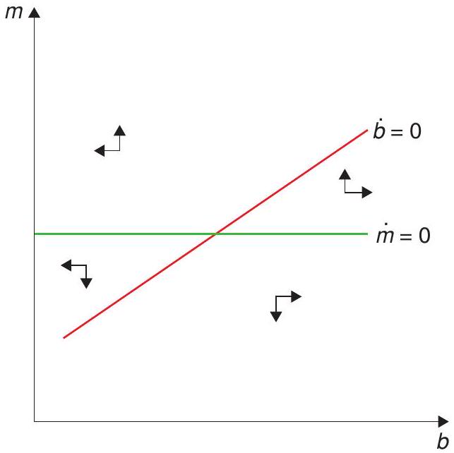
Equations (19.46) and (19.47) will be the dynamic system, which we will use to discuss our results. It is easy to see that the \(\dot{b}\) equation slopes upwards and that the \(\dot{m}\) is an horizontal line. The dynamics are represented in Figure 19.4. A reduction in \(\sigma\) shifts both curves upwards.
Notice that the system is unstable. But \(b\) is not a jump variable. The system reaches stability only if the rate of money growth is such that it can finance the deficit stabilising the debt dynamics. It is the choice of money growth that will take us to the equilibrium. \(b\) here is not the decision variable.
Our exercise considers the case where the rate of growth of money falls for a certain period of time after which it moves to the value needed to keep variables at their steady state. This exercise represents well the case studied by Sargent and Wallace.
To analyse this we first compute all the steady state combinations of \(m\) and \(b\) for different values of \(\sigma\). Making \(\dot{b}\) and \(\dot{m}\) equal to zero in (19.46) and (19.47) and substituting \(\sigma\) in (19.46) using (19.47), we get
\[ b=\frac{m v^{\prime}(m)}{\rho}-m-\frac{D}{\rho} . \tag{19.48}\]
This is the SS locus in Figure 19.5. We know that eventually the economy reverts to a steady state along this line. To finalize the analysis, show that the equation for the accumulation of assets can be written as
\[ \dot{a}_{t}=\rho a_{t}-v^{\prime}\left(m_{t}\right) m_{t}+D . \tag{19.49}\]
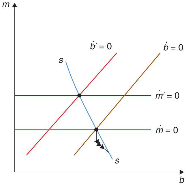
notice, however, that if \(\dot{a}=0\) this equation coincides with (19.48). This means that above the steady states locus the dynamic paths have a slope that is less than one (so that the sum of \(m\) and \(b\) grows as you move) and steeper than one below it (so that the total value of assets falls).
We have now the elements to discuss our results. Consider first the case where \(v(m)=\log (m)\). In this case the inflation tax is constant and independent of the inflation rate. Notice that this implies from (19.44) that the \(\dot{b}=0\) line is vertical. In this case, the reduction in the growth rate of money implies a jump to the lower inflation rate, but the system remains there and there is no unpleasant monetary arithmetic. A lowering of the rate of growth of money, does not affect the collection of the inflation tax and thus does not require more debt financing, so the new lower inflation equilibrium can sustain itself, and simply jumps back to the original point when the growth rate of money reverts to its initial value.
Now consider that case where the demand for money is relatively inelastic, which implies that, in order to increase seigniorage, a higher inflation rate is required and the slope of the SS curve is negative.5 Now the policy of reducing seigniorage collection for some time will increase inflation in the long run as a result of the higher level of debt. This is the soft version of the Sargent-Wallace result.
But the interesting question is whether it may actually increase inflation even in the short run, something we call the hard version of the unpleasant monetarist arithmetic, or, in Drazen’s words, the spectacular version.
Whether this is the case will depend on the slope of the SS curve. If the curve is flat then a jump in \(m\) is required to put the economy on a path to a new steady state. In this case, only the soft, and not the hard, version of the result holds (an upwards jump in \(m\) happens only if inflation falls). However, if the SS curve is steeper than negative one (the case drawn in (19.5), only a downwards jump in \(m\) can get us to the equilibrium. Now we have Sargent and Wallace’s spectacular, unpleasant monetary result: lowering the rate of money growth can actually increase the inflation rate in the short run! The more inelastic money demand, then the more likely this is to be in this case.
Of course these results do not carry to all bond issues. If, for example, a central bank sells bonds \(B_{t}\) to buy foreign reserves \(R e_{t}\) (where \(e_{t}\) is the foreign currency price in domestic currency units), the central bank income statement changes by adding an interest cost \(i \Delta B_{t}\) but also adds a revenue equal
to \(i^{*} R e_{t}\) where \(i\) and \(i^{*}\) stand for the local and foreign interest rates. If \(\Delta B=R e\), to the extent that \(i=i^{*}+\frac{\dot{e}}{e}\) (uncovered interest parity), there is no change in net income, and therefore no change in the equilibrium inflation rate.
This illustrates that the Sargent-Wallace result applies to bond sales that compensate money printed to finance the government (i.e. with no backing). In fact, in Chapter 21 we will discuss the policy of quantitative easing, a policy in which Central Banks issue substantial amount of liquidity in exchange for real assets, such as corporate bonds, and other financial instruments, finance with interest bearing reserves. To the extent that these resources deliver an equilibrium return, they do not change the monetary equilibrium.
19.3.4 Pleasant monetary arithmetic
Let’s imagine now that the government needs to finance a certain level of government expenditure, but can choose the inflation rates over time. What would be the optimal path for the inflation tax? To find out, we assume a Ramsey planner that maximises consumer utility, internalising the optimal behaviour of the consumer to the inflation tax itself, much in the same way we did in the previous chapter in our discussion of optimal taxation; and, of course, subject to its own budget constraint.6 The problem is then to maximise
\[ \int_{0}^{\infty}\left[u(y)+v\left(L\left(i_{t}, y\right)\right)\right] e^{-\rho t} d t \tag{19.50}\]
where we replace \(c\) for \(y\) and \(m_{t}\) for \(L\left(i_{t}, y\right)\), as per the results of the Sidrauski model. The government’s budget constraint is
\[ \dot{a}_{t}=\rho a_{t}-i_{t} m_{t}+d_{t}, \tag{19.51}\]
where \(a_{t}=\frac{B_{t}+M_{t}}{P_{t}}\) is the real amount of liabilities of the government, \(d_{t}\) is the government deficit and we’ve replaced \(r=\rho\). The Ramsey planner has to find the optimal sequence of interest rates, that is, of the inflation rate. The FOCs are
\[ v_{m} L_{i}+\lambda_{t}\left[L\left(i_{t}, y\right)+i_{t} L_{i}\right]=0, \tag{19.52}\]
plus
\[ \dot{\lambda}_{t}=\rho \lambda_{t}-\rho \lambda_{t} . \tag{19.53}\]
The second FOC show that \(\lambda\) is constant. Given this the first FOC shows the nominal interest is constant as well. Optimal policy smooths the inflation tax across periods, a result akin to our tax smoothing result in the previous chapter (if we include a distortion from taxation, we would get that the marginal cost of inflation should equal the marginal cost of taxation, delivering the result that inflation be countercyclical).
Consider what happens if the government faces a decreasing path for government expenditures, that is
\[ d_{t}=d_{0} e^{-\delta t} . \tag{19.54}\]
The solution still requires a constant inflation rate but now the seigniorage needs to satisfy
\[ \pi^{*} m^{*}=\rho b_{0}+\rho \frac{d_{0}}{\rho+\delta} . \tag{19.55}\]
Integrating (19.51) gives the solution for \(a_{t}\)
\[ b_{t}=\frac{\pi^{*} m^{*}}{\rho}-\frac{d_{0}}{\rho+\delta} e^{-\delta t} . \tag{19.56}\]
Notice that debt increases over time: the government smoothes the inflation tax by running up debt during the high deficit period. This debt level is higher, of course, relative to a policy of financing the deficit with inflation in every period (this would entail a decreasing inflation path pari passu with the deficit). At the end, the level of debt is higher under the smoothing equilibrium than under the policy of full inflation financing, leading to higher steady state inflation. This is the monetaristic arithmetic at work. However, far from being unpleasant, this is the result of an optimal program. The higher long run inflation is the cost of smoothing the inflation in other periods.
19.4 The costs of inflation
The Sidrauski model shows that inflation does not affect the equilibrium. But somehow we do not believe this result to be correct. On the contrary, we believe inflation is harmful to the economy. In their celebrated paper, Bruno and Easterly (1996) found that, beyond a certain threshold inflation was negatively correlated with growth, a view that is well established among practicioners of monetary policy. This result is confirmed by the literature on growth regressions. Inflation always has a negative and significant effect on growth. In these regressions it may very well be that inflation is capturing a more fundamental weakness as to how the political system works, which may suggest that for these countries it is not as simple as “choosing a better rate of inflation”.
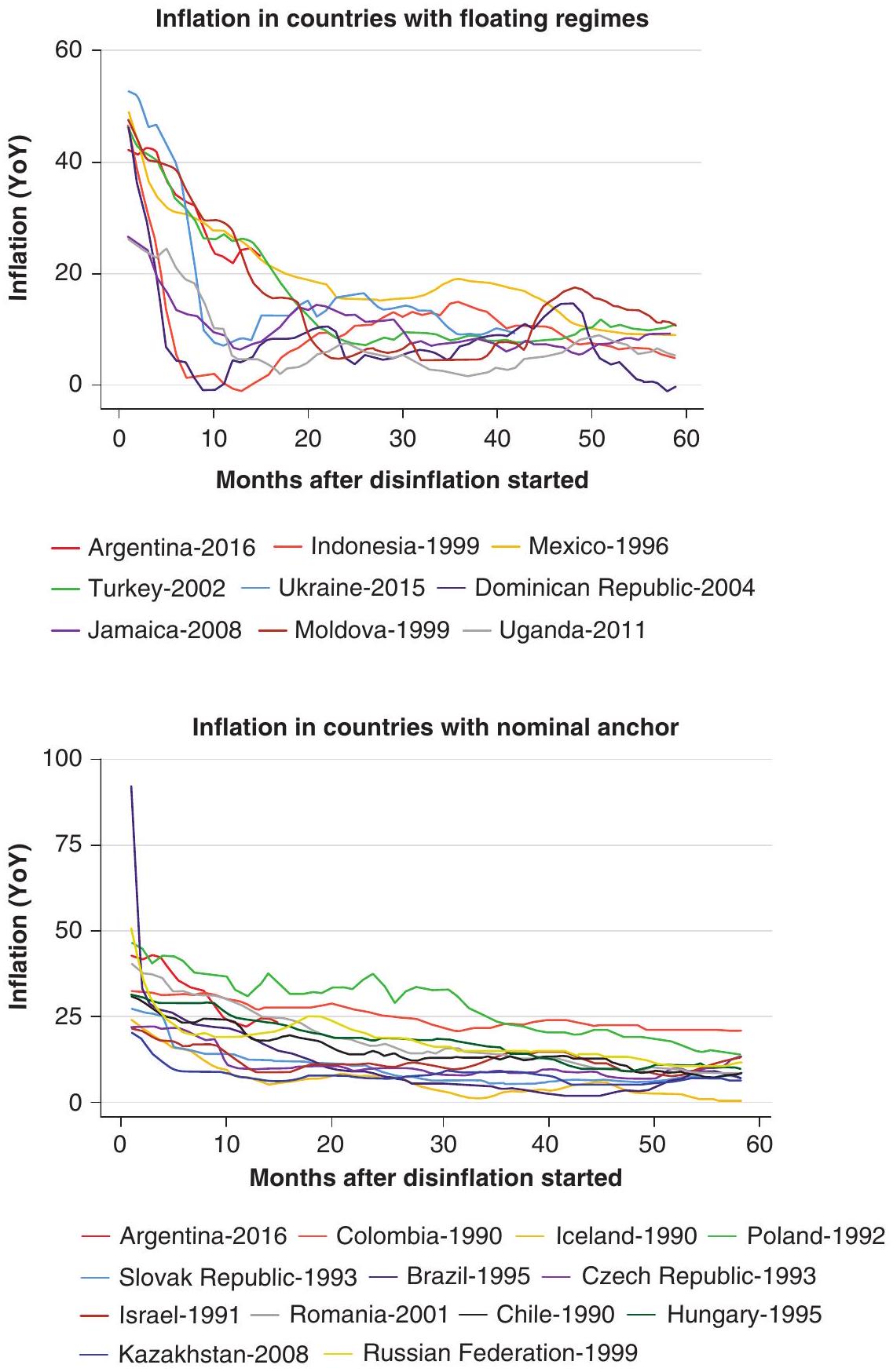
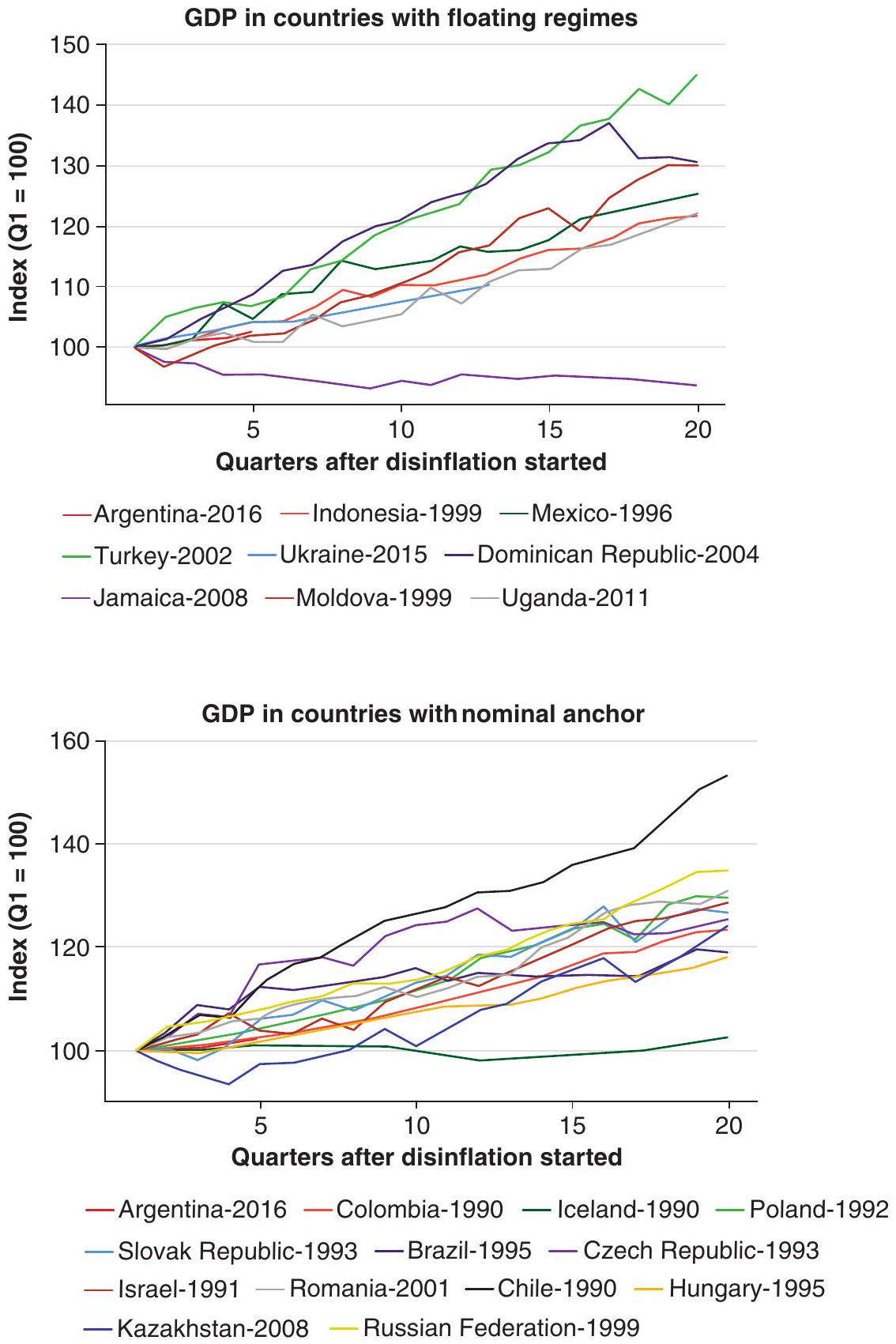
However, to make the point on the costs of inflation more strongly, we notice that even disinflation programs are expansionary. This means that the positive effects of lowering inflation are strong, so much so that they even undo whatever potential costs a disinflation may have. Figures 19.6 and 19.7 show all recent disinflation programs for countries that had reached an inflation rate equal to or higher than 20% in recent years. The figure is split in two panels, those countries that implemented disinflation with a floating regime and those that used some kind of nominal anchor (typically the exchange rate), and shows the evolution of inflation (monthly) in 19.6 and GDP (quarterly) in 19.7 since the last time they reached 20% anual inflation. The evidence is conclusive: disinflations are associated with higher growth.
So what are these costs of inflation that did not show up in the Sidrauski model? There has been a large literature on the costs of inflation. Initially, these costs were associated with what were dubbed shoe-leather costs: the cost of going to the bank to get cash (the idea is that the higher the inflation, the lower your demand for cash, and the more times you needed to go to the bank to get your cash). This was never a thrilling story (to say the least), but today, with electronic money and credit cards, simply no longer makes any sense. On a more benign note we can grant it tries to capture all the increased transaction costs associated with running out (or low) of cash.
Other stories are equally disappointing. Menu costs (the idea that there are real costs of changing prices) is as uneventful as the shoe-leather story. We know inflation distorts tax structures and redistributes incomes across people (typically against the poorest in the population), but while these are undesirable consequences they on their own do not build a good explanation for the negative impact of inflation on growth.
19.4.1 The Tommasi model: Inflation and competition
So the problem with inflation has to be significant and deep. An elephant in the room that seems difficult to see. Tommasi (1994) provides what we believe is a more plausible story based on the role of inflation in messing up the price system. Tommasi focuses on a well-known fact: increases in inflation increase the volatility in relative prices (this occurs naturally in any model where prices adjust at different times or speed). Tommasi argues that relative prices changes, not only generate economic inefficiencies but also change the relative power of sellers and purchasers pushing the economy away from its competitive equilibrium. To see this, let’s draw from our analysis of search discussed in Chapter 16.
Imagine a consumer that is searching for a low price. Going to a store implies finding a price, the value of which can be described by
\[ r W(p)=(\bar{x}-p)+\rho[U-W(p)] . \tag{19.57}\]
Having a price implies obtaining a utility \(\bar{x}-p\). If relative prices were stable, the consumer could go back to this store and repurchase, but if relative prices change, then this price is lost. This occurs with probability \(\rho\). If this event occurs, the consumer is left with no offer (value \(U\) ). The \(\rho\) parameter will change with inflation and will be our object of interest. If the consumer has no price, he needs to search for a price with cost \(C\) and value \(U\) as in
\[ r U=-C+\alpha \int_{0}^{\infty} \max (0, W(p)-U) d F(p) \tag{19.58}\]
Working analogously as we did in the case of job search, remember that the optimal policy will be determined by a reservation price \(p_{R}\). As this reservation price is the one that makes the customer indifferent between accepting or not accepting the price offered, we have that \(r W\left(p_{R}\right)=\bar{x}-p_{R}=r U\), which will be handy later on. Rewrite (19.57) as
\[ W(p)=\frac{\bar{x}-p+\rho U}{r+\rho} . \tag{19.59}\]
Subtracting \(U\) from both sides (and using \(r U=\bar{x}-p_{R}\) ), we have
\[ W(p)-U=\frac{\bar{x}-p+\rho U}{r+\rho}-U=\frac{\bar{x}-p-r U}{r+\rho}=\frac{p_{R}-p}{r+\rho} . \tag{19.60}\]
We can now replace \(r U\) and \(W(p)-U\) in (19.58) to obtain
\[ \bar{x}-p_{R}=-C+\frac{\alpha}{r+\rho} \int_{0}^{p_{R}}\left(p_{R}-p\right) d F(p), \tag{19.61}\]
or, finally,
\[ p_{R}=C+\bar{x}-\frac{\alpha}{r+\rho} \underbrace{\int_{0}^{p_{R}}\left(p_{R}-p\right)}_{(+)} d F(p) \tag{19.62}\]
The intuition is simple. The consumer is willing to pay up to his valuation of the good \(\bar{x}\) plus the search cost \(C\) that can be saved by purchasing this unit. However, the reservation price falls if there is expectation of a better price in a new draw.
The equation delivers the result that if higher inflation implies a the higher \(\rho\), then the higher is the reservation price. With inflation, consumers search less thus deviating the economy from its competitive equilibrium.
Other stories have discussed possible other side effects of inflation. There is a well documented negative relation between inflation and the size of the financial sector (see for example Levine and Renelt (1991) and Levine and Renelt (1992)). Another critical feature is the fact that high inflation implies that long term nominal contracts disappear, a point which becomes most clear if inflation may change abruptly. Imagine a budget with an investment that yields a positive or negative return \(x\) or \(-x\), in a nominal contract this may happen if inflation moves strongly. Imagine that markets are incomplete and agents cannot run negative net worth (any contract which may run into negative wealth is not feasible). The probability of eventually running into negative wealth increases with the length of the contract.7 The disappearance of long term contracts has a negative impact on productivity.
19.4.2 Taking stock
We have seen how money and inflation are linked in the long run, and that a simple monetary model can help account for why central banks would want to set inflation at a low level. We haven’t really talked about the short run, in fact, in our model there are no real effects of money or monetary policy. However, as you anticipate by now, this is due to the fact that there are no price rigidities. To the extent that prices are flexible in the long run, the main concern of monetary policy becomes dealing with inflation, and this is how the practice has evolved in recent decades. If there are rigidities, as we have seen previously, part of the effect of monetary policy will translate into output, and not just into the price dynamics. It is to these concerns that we turn in the next chapter.
References
Bruno, M. & Easterly, W. (1996). Inflation and growth: In search of a stable relationship. Federal Reserve Bank of St. Louis Review, 78(May/June 1996).
Cagan, P. (1956). The monetary dynamics of hyperinflation. Studies in the Quantity Theory of Money.
Colacelli, M. & Blackburn, D. J. (2009). Secondary currency: An empirical analysis. Journal of Monetary Economics, 56(3), 295-308.
de Carvalho Filho, I. & Chamon, M. (2012). The myth of post-reform income stagnation: Evidence from Brazil and Mexico. Journal of Development Economics, 97(2), 368-386.
Drazen, A. (1985). Tight money and inflation: Further results. Journal of Monetary Economics, 15(1), 113-120.
Gluzmann, P. & Sturzenegger, F. (2018). An estimation of CPI biases in Argentina 1985-2005 and its implications on real income growth and income distribution. Latin American Economic Review, 27(1), 8.
Kiguel, M. A. & Neumeyer, P. A. (1995). Seigniorage and inflation: The case of Argentina. Journal of Money, Credit and Banking, 27(3), 672-682.
Kiyotaki, N. & Wright, R. (1989). On money as a medium of exchange. Journal of Political Economy, 97(4), 927-954.
Levine, R. & Renelt, D. (1991). Cross-country studies of growth and policy: Methodological, conceptual, and statistical problems (Vol. 608). World Bank Publications.
Levine, R. & Renelt, D. (1992). A sensitivity analysis of cross-country growth regressions. The American Economic Review, 942-963.
Neumeyer, P. A. (1998). Inflation-stabilization risk in economies with incomplete asset markets. Journal of Economic Dynamics and Control, 23(3), 371-391.
Obstfeld, M. & Rogoff, K. (1983). Speculative hyperinflations in maximizing models: Can we rule them out? Journal of Political Economy, 91(4), 675-687.
Sargent, T. J. & Wallace, N. (1981). Some unpleasant monetarist arithmetic. Federal Reserve Bank of Minneapolis Quarterly Review, 5(3), 1-17.
Sidrauski, M. (1967). Rational choice and patterns of growth in a monetary economy. The American Economic Review, 57(2), 534-544.
Sims, C. A. (2016). Fiscal policy, monetary policy and central bank independence. https://bit.ly/3BmMJYE.
Sturzenegger, F. A. (1994). Hyperinflation with currency substitution: Introducing an indexed currency. Journal of Money, Credit and Banking, 26(3), 377-395.
Tommasi, M. (1994). The consequences of price instability on search markets: Toward understanding the effects of inflation. The American Economic Review, 1385-1396.
Uribe, M. (2016). Is the monetarist arithmetic unpleasant? (tech. rep.). National Bureau of Economic Research.
de Carvalho Filho and Chamon (2012) find a 4.5% annual bias for Brazil in the 80s. Gluzmann and Sturzenegger (2018) find a whopping \(7 \%\) bias for 85-95 in Argentina, and \(1 \%\) for the period 95-2005.↩︎
You may know this already, but the Laffer curve describes the evolution of tax income as you increase the tax rate. Starts at zero when the tax rate is zero, and goes back to zero when the tax rate is 100%, as probably at this high rates the taxable good has disappeared. Thus, there is a range of tax rates where increasing the tax rate decreases tax collection income.↩︎
See Kiguel and Neumeyer (1995).↩︎
If \(y=c+g\) then \(y-c=g\), and as there are no tax resources, it indicates the value of the deficit.↩︎
We disregard the equilibria where the elasticity is so high that reducing the rate of money growth increases the collection of the inflation tax. As in the previous section, we disregard these cases because we typically find the inflation tax to operate on the correct side of the Laffer curve.↩︎
This section follows Uribe (2016).↩︎
For a contract delivering a positive or negative return \(x\) with equal probabilities in each period, the possibility of the contract eventually hitting a negative return is .5 if it lasts one period and \(.5+\sum_{3,5, \ldots}^{\infty} \frac{1}{n+1} \frac{(n-2)!!}{(n-1)!!}\) if it lasts \(n\) periods. This probability is bigger than \(75 \%\) after nine periods, so, quickly long term contracts become unfeasible. See Neumeyer (1998) for a model along these lines.↩︎