15 (New) Keynesian theories of fluctuations: A primer
Keynesian thinking starts from a different viewpoint, at least compared with that of the RBC approach, regarding the functioning of markets. In this perspective, output and employment fluctuations indicate that labour markets, good markets, or both, are not working, leading to unnecessary unemployment. The idea is that, at least in some circumstances, the economy is demand-constrained (rather than supply-constrained), so that the challenge is to increase expenditure. If that could be done, then supply will respond automatically. (This is Keynes’s Principle of Effective Demand.1 ) As a result, Keynesian models focus on aggregate demand management as opposed to supply-side policies. Later on in the book we will discuss specifically the role of fiscal and monetary policy in aggregate demand, but in this chapter we need to understand the framework under which this aggregate demand management matters.
Of course there is a lot of controversy among economists as to how is it possible that a situation where markets fail to clear may persist over time. Why is there unemployment? Can unemployment be involuntary? If it is involuntary, why don’t people offer to work for less? Why are prices rigid? Why can’t firms adjust their prices? How essential is price fixing in comparison with distortions on the labour market? And, in this setup, do consumers satisfy their intertemporal budget constraints?
These are difficult questions that have led to a large amount of literature trying to develop models with Keynesian features in a microfounded equilibrium framework with rational expectations. This line of work that has been dubbed New Keynesianism, emerged as a reaction to the challenge posed by the New Classical approach. Over time, and as New Classical thinking evolved into the RBC approach, the literature coalesced around the so-called DSGE models - with the New Keynesian literature building on these models while adding to them one or many market imperfections.
In any event, this is a very broad expanse of literature that we will not be able to review extensively here. We will thus focus on three steps. First, we will revisit the standard IS-LM model. This model captures the essence (or so most economists think) of the Keynesian approach, by imposing the assumption of price rigidities, which gives rise to the possibility of aggregate demand management. This simple approach, however, begs the question of what could explain those rigidities. Our second step therefore will be to provide a brief discussion of possible microfoundations for them. There may be many reasons for why a nominal price adjustment is incomplete: long-term client relationships, staggered price adjustment, long-term contracts, asymmetric information, menu costs, etc. Not all of
these lead to aggregate price rigidities, but we will not get into these details here. We will instead focus on a model where asymmetric information is the reason for incomplete nominal adjustments. This microfounded model highlights, in particular, the role of expectations in determining the reach of aggregate demand management.2 Last but not least, we will see how these microfoundations combine to give rise to the modern New Keynesian DSGE models, which reinterpret the Keynesian insights in a rather different guise, and constitute the basis of most of macroeconomic policy analysis these days. (We include at the end of the book an appendix that takes you through the first steps needed so that you can run a DSGE model of your own!)
With at least some analytical framework that makes sense of the Keynesian paradigm and its modern interpretation, in later chapters we will discuss the mechanisms and policy levers for demand management, with an emphasis on monetary policy and fiscal policy.
15.1 Keynesianism 101: IS-LM
We revisit the basic version of the Keynesian model that should be familiar from undergraduate macroeconomics: the IS-LM model.
In 1937, J.R. Hicks3 provided a theoretical framework that can be used to analyse the General Theory Keynes had published the previous year. Keynes’s book had been relatively hard to crack, so the profession embraced Hicks’s simple representation that later became known as the IS-LM, model and went on to populate intermediate macro textbooks ever since (Hicks won the Nobel Prize in Economics in 1972 for this work). While much maligned in many quarters (particularly because of its static nature and lack of microfoundations), this simple model (and its open-economy cousin, the Mundell-Fleming model) is still very much in the heads of policy makers.
The model is a general equilibrium framework encompassing three markets: goods, money and bonds, though only two are usually described as the third will clear automatically if the other two do (remember Walras Law from micro!). It is standard to represent the model in terms of interest rates and output, and to look at the equilibrium in the money and goods market. The corresponding equations are:
A money market equilibrium locus called the \(L M\) curve:
\[ \frac{M}{P}=L\left(\begin{array}{c} (-) \\ i, \end{array} \frac{(+)}{Y}\right), \tag{15.1}\]
and a goods market equilibrium called the \(I S\) curve:
\[ Y=A(\stackrel{(-)}{r}, \underbrace{\stackrel{(+)}{Y}}_{<1}, \stackrel{(+)}{\text { ( }+)} \text {, } \stackrel{(+)}{\text { iscal }}, \stackrel{(+)}{R E R}) \tag{15.2}\]
where Fiscal stands for government expenditures and RER for the real exchange rate, or, alternatively,
\[ Y=A(\stackrel{(-)}{r}, \stackrel{(+)}{\text {, Fiscal, }} \stackrel{(+)}{R E R}) . \tag{15.3}\]
Finally, a relationship between nominal and real interest rates:
\[ r=i-\pi^{e} . \tag{15.4}\]
15.1.1 Classical version of the IS-LM model
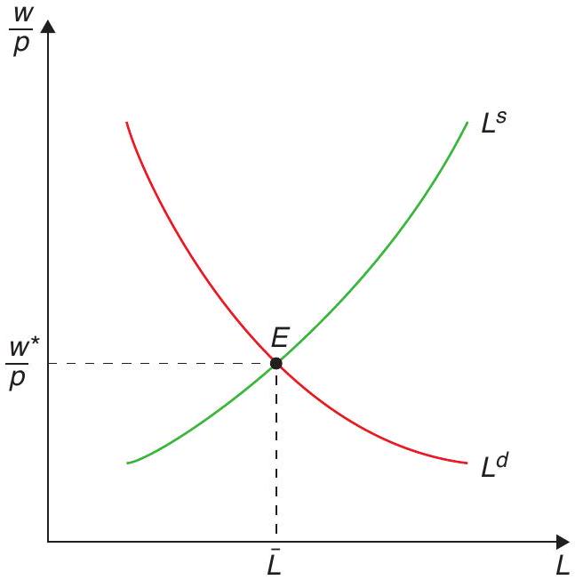
In the classical version of the model, all prices are flexible, and so are real wages. Thus the labour market clears fixing the amount of labour as in Figure 15.1.
With full employment of labor and capital, output is determined by the supply constraint and becomes an exogenous variable, which we will indicate with a bar:
\[ \bar{Y}=F(K, \bar{L}) . \tag{15.5}\]
The \(I S\), can then be used to determine \(r\) so that savings equals investment ( \(S=I\), thus the name of the curve). The nominal interest rate is just the real rate plus exogenous inflation expectations (equivalent to the expected growth rate of prices). With \(Y\) and \(i\) fixed, then the \(L M\) determines the price level \(P\) given a stock of nominal money:
\[ P=\frac{\bar{M}}{L(i, \bar{Y})}, \tag{15.6}\]
which is an alternative way of writing the quantity equation of money:
\[ M V=P Y . \tag{15.7}\]
In short, the structure of the model is such that the labor market determines the real wage and output. The IS determines the real and nominal interest rate, and the money market determines the price level.
This is typically interpreted as a description of the long run, the situation to which the economy gravitates at any given moment. The idea is that prices eventually adjust so that supply ends up determining output. That is why we ignored aggregate demand fluctuations when discussing long-run growth. There we concentrated on the evolution of the supply capacity. In the classical version of the model (or in the long run) that supply capacity determines what is produced.
15.1.2 The Keynesian version of the IS-LM model
However, as Keynes famously quipped, in the long run, we will all be dead. In the short run, the Keynesian assumption is that prices are fixed or rigid, and do not move to equate supply and demand:
\[ P=\bar{P}, \tag{15.8}\]
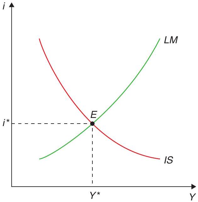
so now the \(I S\) and \(L M\) curves jointly determine \(Y\) and \(i\) as in Figure 15.2.
Notice that \(Y\) is determined without referring to the labour market, so the level of labour demand may generate involuntary unemployment.
It is typical in this model to think of the effects of monetary and fiscal policy by shifting the IS and LM curves, and you have seen many such examples in your intermediate macro courses. (If you don’t quite remember it, you may want to get a quick refresher from any undergraduate macro textbook you prefer.) We will later show how we can think more carefully about these policies, in a dynamic, microfounded context.
15.1.3 An interpretation: The Fed
Is the model useful? Yes, because policy makers use it. For example, when the Fed talks about expanding or contracting the economy it clearly has a Keynesian framework in mind. It is true that the Fed does not typically operate on the money stock, but one way of thinking about how the Fed behaves is to think of it as determining the interest rate and then adjusting the money supply to the chosen rate (money becomes somewhat endogenous to the interest rate). In our model, \(i\) becomes exogenous and \(M\) endogenous as in Figure 15.3:
\[ \frac{M}{\bar{P}}=L(\bar{i}, Y) \tag{15.9}\]
\[ Y=A\left(\bar{i}-\pi^{e}, \text { Fiscal,… }\right) . \tag{15.10}\]
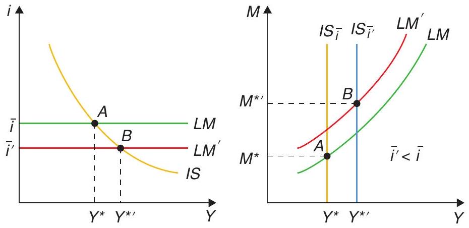
We can represent this using the same \(Y, i\) space, but the LM curve is now horizontal as the Fed sets the (nominal) interest rate. Alternatively, we can think about it in the \(Y, M\) space, since \(M\) is the new endogenous variable. Here we would have the same old \(L M\) curve, but now the IS curve becomes vertical in the \(Y, M\) space. Both represent the same idea: if the Fed wants to expand output, it reduces the interest rate, and this requires an expansion in the quantity of money.
As a side note, you may have heard of the possibility of a liquidity trap, or alternatively, that monetary policy may hit the zero interest lower bound. What does this mean? We can think about it as a situation in which interest rates are so low that the demand for money is infinitely elastic to the interest rate. In other words, because nominal interest rates cannot be negative (after all, the nominal return on cash is set at zero), when they reach a very low point an increase in the supply of money will be hoarded as cash, as opposed to leading to a greater demand for goods and services. In that case, the IS-LM framework tells us that (conventional) monetary policy is ineffective. Simply put, interest rates cannot be pushed below zero!
This opens up a series of policy debates. There are two big questions that are associated with this: 1) Is monetary policy really ineffective in such a point? It is true that interest rate policy has lost its effectiveness by hitting the zero boundary, but that doesn’t necessarily mean that the demand for money is infinitely elastic. The Fed can still pump money into the economy (what came to be known as quantitative easing) by purchasing government (and increasingly private) bonds, and this might still have an effect (maybe through expectations). 2) In this scenario, can fiscal policy be effective? These are debates we’ll come back to in full force in our discussions of fiscal and monetary policy.
15.1.4 From IS-LM to AS-AD
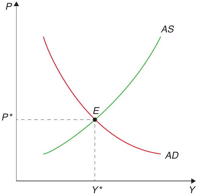
Another way to understand the assumption on price rigidity in generating a role for aggregate demand management is to go from the IS-LM representation to one in which \(P\) is one of the endogenous variables. The LM curve implies that an increase in prices leads to a decrease in the supply of real money balances, which shifts LM to the left. Since IS is not affected, that means that a higher \(P\) leads to a lower level of output \(Y\). This is the aggregate demand (AD) curve in Figure 15.4.
An increase in aggregate demand (through monetary or fiscal policy) will shift the AD curve to the right. The effect that this will have on equilibrium output will depend on the effect of this on prices, which in turn depends on the aggregate supply (AS) of goods and services. The classical case is one in which this supply is independent of the price level - a vertical AS curve. This is the case where prices are fully flexible. The Keynesian case we considered, in contrast, is one in which AS is horizontal ( \(P\) is fixed), and hence the shift in AD corresponds fully to an increase in output. This is an economy that is not supply constrained. In the intermediate case, where prices adjust but not completely, AS is positively sloped, and shifts in aggregate demand will have at least a partial effect on output.
The positively-sloped AS curve is the mirror image of the Phillips curve - the empirical observation of a tradeoff between output/unemployment and prices/inflation. We assume you are familiar with the concept from your intermediate macro courses, and we will get back to that when we discuss the modern New Keynesian approach.
15.2 Microfoundations of incomplete nominal adjustment
We go over a possible explanation for the incomplete adjustment of prices or, more broadly, for why the AS curve may be upward-sloping. We study the Lucas model of imperfect information, which illustrates how we can solve models with rational expectations.
We have now reestablished the idea that, if prices do not adjust automatically, aggregate demand management can affect output and employment. The big question is, what lies behind their failure to adjust? Or, to put it in terms of the AS-AD framework, we need to understand why the AS curve is positively sloped, and not vertical. Old Keynesian arguments were built on things such as backward-looking (adaptive) expectations, money illusion, and the like. This, in turn, rubbed more classical-minded economists the wrong way. How can rational individuals behave in such a way? Their discomfort gained traction when the Phillips curve tradeoff seemed to break down empirically in the late 1960s and early 1970s. The model is also useful from a methodological point of view: it shows how a rational expectations model is solved. In other words, it shows how we use the model to compute the expectations that are an essential piece of the model itself. Let’s see!
15.2.1 The Lucas island model
The challenge to Keynesian orthodoxy, and hence the initial push from which modern Keynesian theories were built, took the shape of the pioneering model by Lucas (1973) - part of his Nobel-winning contribution. He derived a positively-sloped AS curve in a model founded at the individual level, and where individuals had rational expectations. This model also more explicit the role of expectations in constraining aggregate demand policy. The key idea was that of imperfect information: individuals can observe quite accurately the prices of the goods they produce or consume most often, but they cannot really observe the aggregate price level. This means that, when confronted with a higher demand for the good they produce, they are not quite sure whether that reflects an increase in its relative price - a case in which they should respond by increasing their output - or simply a general increase in prices - a case in which they should not respond with quantities, but just adjust prices. We will see that rational expectations implies that individuals should split the difference and attribute at least part of the increase to relative prices. (How much so will depend on how often general price increases occur.) This yields the celebrated Lucas supply curve, a positively-sloped supply curve in which output increases when the price increases in excess of its expected level.
The model is one with many agents (Lucas’s original specification places each person on a different island, which is why the model is often referred to as the Lucas island model). Each agent is a consumer-producer that every period sees a certain level of demand. The basic question is to figure out if an increase in demand is an increase in real demand, which requires an increase in production levels, or if it is simply an increase in nominal demand, to which the optimal response is just an increase in prices. The tension between these two alternatives is what will give power to the model. In order to solve the model we will start with a specification with perfect information and, once this benchmark case is solved, we will move to the case of asymmetric information, which is where all the interesting action is.
15.2.2 The model with perfect information
The representative producer of good \(i\) has production function
\[ Q_{i}=L_{i}, \tag{15.11}\]
so that her feasible consumption is
\[ c_{i}=\frac{P_{i} Q_{i}}{P} . \tag{15.12}\]
Utility depends (positively) on consumption and (negatively) on labour effort. Let’s assume the specification
\[ u_{i}=c_{i}-\frac{1}{\gamma} L_{i}^{\gamma} \quad \gamma>1 . \tag{15.13}\]
If \(P\) is known (perfect information), the problem is easy; the agent has to maximize her utility (15.13) with respect to her supply of the good (which is, at the same time, her supply of labour). Replacing (15.11) and (15.12) in (15.13) gives
\[ u_{i}=\frac{P_{i} L_{i}}{P}-\frac{1}{\gamma} L_{i}^{\gamma} . \tag{15.14}\]
The first order condition for \(L\) is
\[ \frac{P_{i}}{P}-L_{i}^{\gamma-1}=0, \tag{15.15}\]
which can be written as a labour supply curve
\[ L_{i}=\left(\frac{P_{i}}{P}\right)^{\frac{1}{\gamma-1}}, \tag{15.16}\]
or, if expressed in logs (denoted in lower case letters), as
\[ l_{i}=\left(\frac{1}{\gamma-1}\right)\left(p_{i}-p\right) . \tag{15.17}\]
As expected, supply (production) increases with the relative price of the good.
Next, we need to think about demand for every good \(i\), and about aggregate demand. The former takes a very simple form. It can be derived from basic utility but no need to do so here as the form is very intuitive. Demand depends on income, relative prices, and a good-specific taste shock - in log format it can be written as
\[ q_{i}=y+z_{i}-\eta\left(p_{i}-p\right) \quad \eta>0, \tag{15.18}\]
where \(y\) is average income and \(p\) is the average price level. The taste shock \(z_{i}\) is assumed to affect relative tastes, hence it averages to zero across all goods. It is also assumed to be normally distributed, for reasons that will soon be clear, with variance \(v_{z}\).
How about aggregate demand? We will assume that there is an aggregate demand shifter, a policy variable we can control, which in this case will be \(m\). It can be anything that shifts the AD curve within the AS-AD framework developed above, but to fix ideas we can think about monetary policy. To introduce, it consider a money demand function in log form:
\[ y=m-p . \tag{15.19}\]
We assume that \(m\) is also normally distributed, with mean \(E(m)\) and variance \(v_{m}\).
Equilibrium
To find the equilibrium we make demand equal to supply for each good. This is a model with market clearing and where all variables, particularly \(p\), are known.
\[ \left(\frac{1}{\gamma-1}\right)\left(p_{i}-p\right)=y+z_{i}-\eta\left(p_{i}-p\right), \tag{15.20}\]
from which we obtain the individual price
\[ p_{i}=\frac{(\gamma-1)}{1+\eta \gamma-\eta}\left(y+z_{i}\right)+p, \tag{15.21}\]
and from which we can obtain the average price. Averaging (15.21) we get
\[ p=\frac{(\gamma-1)}{(1+\eta \gamma-\eta)} y+p \tag{15.22}\]
which implies
\[ y=0 . \]
You may find it strange, but it is not: remember that output is defined in logs. Replacing the solution for output in (15.19) we get that
\[ p=m, \tag{15.23}\]
i.e. that prices respond fully to monetary shocks. In other words, the world with perfect information is a typical classical version with flexible prices and where aggregate demand management has no effect on real variables and full impact on nominal variables.
15.2.3 Lucas’ supply curve
When there is imperfect information, each producer observes the price of her own good, \(p_{i}\), but cannot observe perfectly what happens to other prices. She will have to make her best guess as to whether a change in her price represents an increase in relative prices, or just a general increase in the price level. In other words, labour supply will have to be determined on the basis of expectations. Because we assume rational expectations, these will be determined by the mathematical expectation that is consistent with the model - in other words, individuals know the model and form their expectations rationally based on this knowledge.
Denote relative prices as \(r_{i}=\left(p_{i}-p\right)\), then the analog to (15.17) is now4
\[ l_{i}=\left(\frac{1}{\gamma-1}\right) E\left(r_{i} \mid p_{i}\right) . \tag{15.24}\]
It so happens that if the distribution of the shocks \(z_{i}\) and \(m\) is jointly normal, then so will be \(r_{i}, p_{i}\), and \(p\). Since \(r_{i}\) and \(p_{i}\) are jointly normally distributed, a result from statistics tells us that the conditional expectation is a linear function
\[ E\left(r_{i} \mid p_{i}\right)=\alpha+\beta p_{i} . \tag{15.25}\]
More specifically, in this case, we have what is called a signal extraction problem, in which one variable of interest \(\left(r_{i}\right)\) is observed with noise. What you observe \(\left(p_{i}\right)\) is the sum of the signal you’re interested in \(\left(r_{i}\right)\), plus noise you don’t really care about \((p)\). It turns out that, with the assumption of normality, the solution to this problem is
\[ E\left(r_{i} \mid p_{i}\right)=\frac{v_{r}}{v_{r}+v_{p}}\left(p_{i}-E(p)\right), \tag{15.26}\]
where \(v_{r}\) and \(v_{p}\) are the variances of relative price and general price level, respectively. (They are a complicated function of \(v_{z}\) and \(v_{m}\).) This expression is very intuitive; if most of the variance comes from the signal, your best guess is that a change in \(p_{i}\) indicates a change in relative prices. Substituting in (15.24) yields
\[ l_{i}=\left(\frac{1}{\gamma-1}\right) \frac{v_{r}}{v_{r}+v_{p}}\left(p_{i}-E(p)\right) . \tag{15.27}\]
Aggregating over all the individual supply curves, and defining
\[ b=\frac{1}{\gamma-1} \frac{v_{r}}{v_{r}+v_{p}} \tag{15.28}\]
we have that
\[ y=b(p-E(p)), \tag{15.29}\]
which is actually a Phillips curve, as you know from basic macro courses.
This became known as the Lucas supply curve. Note that this is a positively-sloped supply curve, in which output increases when the price increases in excess of its expected level. Why is it so? Because when facing such an increase, imperfectly informed producers rationally attribute some of that to an increase in relative prices. It also says that labour and output respond more to price changes if the relative relevance of nominal shocks is smaller. Why is this? Because the smaller the incidence of nominal shocks, the more certain is the producer that any price shock she faces is a change in real demand.
Solving the model
We know from the AS-AD framework that, with a positively-sloped supply curve, aggregate demand shocks affect equilibrium output. How do we see that in the context of this model? Plugging (15.29) into the aggregate demand equation (15.19) yields
\[ y=b(p-E(p))=m-p, \tag{15.30}\]
that can be used to solve for the aggregate price level and income:
\[ p=\frac{m}{1+b}+\frac{b}{1+b} E(p), \tag{15.31}\]
\[ y=\frac{b m}{1+b}-\frac{b}{1+b} E(p) . \tag{15.32}\]
Now, rational expectations means that individuals will figure this out in setting their own expectations. In other words, we can take the expectations of (15.31) to obtain:5
\[ E(p)=\frac{1}{1+b} E(m)+\frac{b}{1+b} E(p), \tag{15.33}\]
which implies, in turn, that
\[ E(p)=E(m) . \tag{15.34}\]
Using this and the fact that \(m=E(m)+m-E(m)\) we have that
\[ p=E(m)+\frac{1}{1+b}(m-E(m)), \tag{15.35}\]
\[ y=\frac{b}{1+b}(m-E(m)) . \tag{15.36}\]
In short, the model predicts that changes in aggregate demand (e.g. monetary policy) will have an effect on output, but only to the extent that they are unexpected. This is a very powerful conclusion in the sense that systematic policy will eventually lose its effects; people will figure it out, and come to expect it. When they do, they’ll change their behaviour accordingly, and you won’t be able to exploit it. This is at the heart of the famous Lucas critique: as the policy maker acts, the aggregate supply curve will change as a result of that, and you can’t think of them as stable relationships independent of policy.
As we can see, the imperfect information approach highlights the role of expectations in determining the effectiveness of macro policy. This insight is very general, and lies behind a lot of modern policy making: inflation targeting as a way of coordinating expectations, the problem of time inconsistency, etc. In fact, we will soon see that this insight is very much underscored by the modern New Keynesian approach.
15.3 Imperfect competition and nominal and real rigidities
We show that, with imperfect competition and nominal rigidities, there is a role for aggregate demand policy. Imperfect competition means that firms can set prices, and that output can deviate from the social optimum. Nominal rigidities mean that prices fail to adjust automatically. The two combined mean that output can be increased (in the short run), and that doing so can be desirable. We discuss how real rigidities amplify the impact of nominal rigidities.
The Lucas model was seen at the time as a major strike against Keynesian policy thinking. After all, while it illustrates how we can obtain a positively-sloped AS curve from a fully microfounded approach with rational agents, it also fails to provide a justification for systematic macro policy. The New Keynesian tradition emerged essentially as an attempt to reconcile rational expectations and the possibility and desirability of systematic policy.
Consider the desirability: in the Lucas model (or the RBC approach that essentially came out of that tradition), business cycles are the result of optimal responses by individuals to disturbances that occur in this economy, and aggregate demand policy can only introduce noise. If the market equilibrium is socially optimal, then any fluctuation due to aggregate demand shocks is a departure from the optimum, and thus undesirable. The New Keynesian view departs from that by casting imperfect competition in a central role. The key to justifying policy intervention is to consider the possibility that the market-determined level of output is suboptimal, and imperfect competition yields exactly that. In addition, this is consistent with the general impression that recessions are bad and booms are good.
Besides the issue of desirability, we have argued that the Lucas model also implies that systematic policy is powerless; rational agents with rational expectations figure it out, and start adjusting prices accordingly. The second essential foundation of New Keynesian thinking is thus the existence and importance of barriers to price adjustment. Note that this is also related to imperfect competition since price adjustment can only matter if firms are price-setters, which requires some monopoly power. It is not enough to have imperfect competition to have these rigidities, however, as monopolists will also want to adjust prices rather than output in response to nominal shocks.
We thus have to understand how barriers, that are most likely rather small at the micro level, and which have become known in the literature by the catch-all term menu costs, can still have large macroeconomic effects. Do we really think that in the real world the costs of adjusting prices are large enough to lead to sizeable consequences in output?
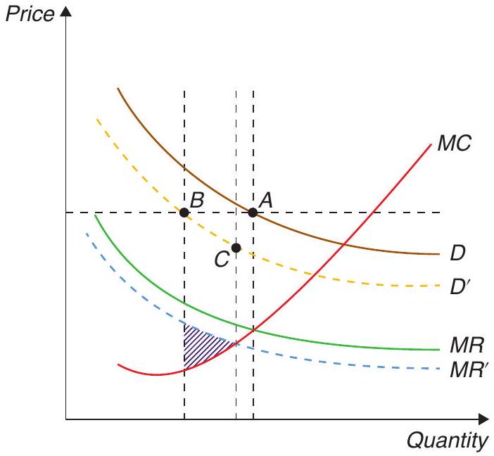
It turns out that the key lies once again with imperfect competition. Consider the effects of a decrease in aggregate demand on the behaviour of monopolist firms, illustrated in Figure 15.5. Taking the behaviour of all other firms as given, this will make any given firm want to set a lower price. If there were no costs of adjustment, the firm would go from point A in Figure 15.5 to point C. If the firm doesn’t adjust at all, it would go to point B. It follows that its gain from adjusting would be the shaded triangle. If the menu cost is greater than that, the firm would choose not to adjust.
But what is the social cost of not adjusting? It is the difference in consumer surplus corresponding to a decrease in quantity from point C to point B. This is given by the area between the demand curve D’ and the marginal cost curve, between B and C. This is much bigger than the shaded triangle! In other words, the social loss is much bigger than the firm’s loss from not adjusting, and it follows that small menu costs can have large social effects.6
Another type of rigidity emphasised by New Keynesians are real rigidities (as distinct from the nominal kind). These correspond to a low sensitivity of the desired price to aggregate output. If the desired price doesn’t change much with a change in output, the incentive to adjust prices will be lower. (Think about the slope of the marginal cost curve in Figure 15.5). If there are no costs of adjustment (i.e. nominal rigidities), that doesn’t matter, of course; but the real rigidities amplify the effect of the nominal ones. These real rigidities could come from many sources, such as the labour market. If labour supply is relatively inelastic (think about low levels of labour mobility, for instance), we would have greater real rigidities. (This actually sets the stage for us to consider our next topic in the study of cyclical fluctuations: labour markets and unemployment.)
In sum, a combination of imperfect competition, nominal rigidities (menu costs), and real rigidities implies that aggregate demand policy is both desirable and feasible. We will now turn to a very brief discussion of how this view of the world has been embedded into full-fledged dynamic stochastic general equilibrium (DSGE) models such as those introduced by the RBC tradition to give birth to the modern New Keynesian view of fluctuations.7
15.4 New Keynesian DSGE models
We express the modern New Keynesian DSGE (NK DSGE) model in its canonical (microfounded) version, combining the New Keynesian IS curve, the New Keynesian Phillips curve, and a policy rule. We show the continuous-time and discrete-time versions of the model.
New Keynesian DSGE models embody the methodological consensus underpinning modern macroeconomics. It has become impossible to work in any self-respecting Central Bank, for instance, without coming across a New Keynesian DSGE model. But modern, state of-the-art DSGE models are very complicated. If you thought that RBC models were already intricate, consider the celebrated NK DSGE model by Smets and Wouters (2003), originally developed as an empirical model of the Euro area. It contains, in addition to productivity shocks, shocks to adjustment costs, the equity premium,
wage markup, goods markup, labor supply, preferences, and the list goes on and on. Another difficulty is that there is little consensus as to which specific model is best to fit real-world fluctuations. So what we do here is consider a few of the key ingredients in NK DSGE models, and explain how they combine into what is often called the canonical New Keynesian model.
15.4.1 The canonical New Keynesian model
We first develop the model in continuous time, which is simpler and allows for the use of phase diagrams, so that we can readily put the model to work and develop some intuition about its operation and dynamics. Later, we turn to discrete time, and write down the version of the model that is most commonly used in practical and policy applications.
The demand side of the canonical New Keynesian model is very simple. We start from our model of consumer optimisation, which by now we have seen many times. You will recall the Euler equation of the representative consumer.
\[ \dot{C}_{t}=\sigma\left(r_{t}-\rho\right) C_{t}, \tag{15.37}\]
where \(C_{t}\) is consumption, \(\sigma>0\) is the elasticity of intertemporal substitution in consumption, and \(\rho\) is the rate of time discounting. In a closed economy with no investment, all output \(Y_{t}\) is consumed. Therefore,
\[ C_{t}=Y_{t}, \tag{15.38}\]
and
\[ \dot{Y}_{t}=\sigma\left(i_{t}-\pi_{t}-\rho\right) Y_{t}, \tag{15.39}\]
where we have used the definition \(r_{t} \equiv i_{t}-\pi_{t}\), and \(i_{t}\) is the nominal interest rate, taken to be exogenous and constant for the time being. If we define the output gap as,
\[ X_{t} \equiv \frac{Y_{t}}{\bar{Y}_{t}}, \tag{15.40}\]
where \(\bar{Y}_{t}\) is the natural or long run level of output, then the output gap evolves according to
\[ \frac{\dot{X}_{t}}{X_{t}}=\frac{\dot{Y}_{t}}{Y_{t}}-g, \tag{15.41}\]
where \(g\) is the percentage growth rate of the natural level of output, assumed constant for now. Finally, letting small-case letters denote logarithms, using the Euler equation (15.39), we have
\[ \dot{x}_{t}=\sigma\left(i_{t}-\pi_{t}-r^{n}\right), \tag{15.42}\]
where \(r^{n} \equiv \rho+\sigma^{-1} g\) is the natural or Wicksellian interest rate, which depends on both preferences and productivity growth. It is the interest rate that would prevail in the absence of distortions, and corresponds to a situation in which output is equal to potential.
This last equation, which we can think of as a dynamic New Keynesian IS equation (or NKIS) summarises the demand side of the model. The NKIS equation says that output is rising when the real interest rate is above its long-run (or natural) level. Contrast this with the conventional IS equation, which says that the level of output (as opposed to the rate of change of output in the equation above) is above its long-run level when the real interest is below its long-run (or natural) level.
The NKIS differs from traditional IS in other important ways. First, it is derived from micro-founded, optimising household behaviour. Second, the relationship between interest rates and output emerges from the behaviour of consumption, rather than investment, as was the case in the old IS. Intuitively, high interest rates are linked to low output now because people decide that it is better to postpone consumption, thereby reducing aggregate demand.
Turn now to the supply side of the model. We need a description of how prices are set in order to capture the presence of nominal rigidities. There are many different models for that, which are typically classified as time-dependent or state-dependent. State-dependent models are those in which adjustment is triggered by the state of the economy. Typically, firms decide to adjust (and pay the menu cost) if their current prices are too far from their optimal desired level. Time-dependent models, in contrast, are such that firms get to adjust prices with the passage of time, say, because there are long-term contracts. This seems slightly less compelling as a way of understanding the underpinnings of price adjustment, but it has the major advantage of being easier to handle. We will thus focus on time-dependent models, which are more widely used.
There are several time-dependent models, but the most popular is the so-called Calvo model. Calvo (1983) assumes that the economy is populated by a continuum of monopolistically-competitive firms. Each of them is a point in the [0, 1] interval, thus making their ’total’ equal to one. The key innovation comes from the price-setting technology: each firm sets its output price in terms of domestic currency and can change it only when it receives a price-change signal. The probability of receiving such a signal \(s\) periods from now is assumed to be independent of the last time the firm got the signal, and given by
\[ \alpha e^{-\alpha s}, \quad \alpha>0 . \tag{15.43}\]
If the price-change signal is stochastically independent across firms, we can appeal to the ’law of large numbers’ to conclude that a share \(\alpha\) of firms will receive the price-change signal per unit of time. By the same principle, of the total number of firms that set their price at time \(s<t\), a share
\[ e^{-\alpha(t-s)} \tag{15.44}\]
will not have received the signal at time \(t\). Therefore,
\[ \alpha e^{-\alpha(t-s)} \tag{15.45}\]
is the share of firms that set their prices at time \(s\) and have not yet received a price-change signal at time \(t>s\).
Next, let \(v_{t}\) be the (log of the) price set by an individual firm (when it gets the signal), and define the (log of the) price level \(p_{t}\) as the arithmetic average of all the prices \(v_{t}\) still outstanding at time \(t\), weighted by the share of firms with the same \(v_{t}\) :
\[ p_{t}=\alpha \int_{-\infty}^{t} v_{s} e^{-\alpha(t-s)} d s . \tag{15.46}\]
It follows that the price level is sticky, because it is a combination of pre-existing prices (which, because they are pre-existing, cannot jump suddenly).
How is \(v_{t}\) set? Yun (1996) was the first to solve the full problem of monopolistically-competitive firms that must set prices optimally, understanding that it and all competitors will face stochastic price-setting signals. Getting to that solution is involved, and requires quite a bit of algebra.8
Here we just provide a reduced form, and postulate that the optimal price \(v_{t}\) set by an individual firm depends on the contemporaneous price level \(p_{t}\), the expected future paths of the (log of) expected relative prices, and of the (log of) the output gap:
\[ v_{t}=p_{t}+\alpha \int_{t}^{\infty}\left[\left(v_{s}-p_{s}\right)+\eta x_{s}\right] e^{-(\alpha+\rho)(s-t)} d s \tag{15.47}\]
where, recall, \(\rho\) is the consumer’s discount rate and \(\eta>0\) is a sensitivity parameter.9 So the relative price the firm chooses today depends on a discounted, probability-weighted average of all future relative prices \(\left(v_{s}-p_{s}\right)\) and all output gaps \(x_{s}\). This is intuitive. For instance, if the output gap is expected to be positive in the future, then it makes sense for the firm to set a higher (relative) price for its good to take advantage of buoyant demand.
Note from this expression that along any path in which the future \(x_{s}\) and \(v_{s}\) are continuous functions of time (which we now assume), \(v_{t}\) is also, and necessarily, a continuous function of time. We can therefore use Leibniz’s rule to differentiate the expressions for \(p_{t}\) and \(v_{t}\) with respect to time, obtaining10
\[ \dot{p}_{t}=\pi_{t}=\alpha\left(v_{t}-p_{t}\right), \tag{15.48}\]
and
\[ \dot{v}_{t}-\dot{p}_{t}=-\alpha \eta x_{t}+\rho\left(v_{t}-p_{t}\right) . \tag{15.49}\]
Combining the two we have
\[ \dot{v}_{t}-\dot{p}_{t}=-\alpha \eta x_{t}+\frac{\rho}{\alpha} \pi_{t} . \tag{15.50}\]
Differentiating the expression for the inflation rate \(\pi_{t}\), again with respect to time, yields
\[ \dot{\pi}_{t}=\alpha\left(\dot{v}_{t}-\dot{p}_{t}\right) . \tag{15.51}\]
Finally, combining the last two expressions we arrive at
\[ \dot{\pi}_{t}=\rho \pi_{t}-\kappa x_{t}, \tag{15.52}\]
where \(\kappa \equiv \alpha^{2} \eta>0\). This is the canonical New Keynesian Phillips curve. In the traditional Phillips curve, the rate of inflation was an increasing function of the output gap. By contrast, in the Calvo-Yun NKPC the change in the rate of inflation is a decreasing function of the output gap! Notice, also that while \(p_{t}\) is a sticky variable, its rate of change \(\pi_{t}\) is not; it is intuitive that \(\pi_{t}\) should be able to jump in response to expected changes in relevant variables.
Solving this equation forward we obtain
\[ \pi_{t}=\int_{t}^{\infty} \kappa x_{s} e^{-\rho(s-t)} d s \tag{15.53}\]
So the inflation rate today is the present discounted value of all the future expected output gaps. The more “overheated” the economy is expected to be in the future, the higher inflation is today.
To complete the supply side of the model we need to specify why the output gap should by anything other than zero - that is, why firms can and are willing to supply more output than their long-term profit maximizing level. The standard story, adopted, for instance, by Yun (1996), has two components. Output is produced using labour and firms can hire more (elastically supplied) labour in the shortrun to enlarge production when desirable. When demand rises (recall the previous section of this
chapter), monopolistically-competitive firms facing fixed prices will find it advantageous to supply more output, up to a point.
This NKPC curve and the dynamic NKIS curve, taken together, fully describe this model economy. They are a pair of linear differential equations in two variables, \(\pi_{t}\) and \(x_{t}\), with \(i_{t}\) as an exogenous policy variable. In this model there is no conflict between keeping inflation low and stabilising output. If \(i=\) \(r^{n}\), then \(\pi_{t}=x_{t}=0\) is an equilibrium. Blanchard and Galí (2007) term this the divine coincidence.
The steady state is
\[ \bar{\pi}=i-r^{n}\left(\text { from } \dot{x}_{t}=0\right) \tag{15.54}\]
\[ \rho \bar{\pi}=\kappa \bar{x}\left(\text { from } \dot{\pi}_{t}=0\right) \tag{15.55}\]
where overbars denote the steady state. If, in addition, we assume \(i=r^{n}\), then \(\bar{\pi}=\bar{x}=0\). In matrix form, the dynamic system is
\[ \left[\begin{array}{c} \dot{\pi}_{t} \\ \dot{x}_{t} \end{array}\right]=\Omega\left[\begin{array}{c} \pi_{t} \\ x_{t} \end{array}\right]+\left[\begin{array}{c} 0 \\ \sigma\left(i-r^{n}\right) \end{array}\right] \tag{15.56}\]
where
\[ \Omega=\left[\begin{array}{cc} \rho & -\kappa \\ -\sigma & 0 \end{array}\right] . \tag{15.57}\]
It is straightforward to see that \(\operatorname{Det}(\Omega)=-\sigma \kappa<0\), and \(\operatorname{Tr}(\Omega)=\rho>0\). It follows that one of the eigenvalues of \(\Omega\) is positive (or has positive real parts) and the other is negative. This means the system exhibits saddle path stability, in other words that for each \(\pi_{t}\) there is a value of \(x_{t}\) from which the system will converge asymptotically to the steady state. But remember that here both \(x\) and \(\pi\) are jump variables! This means that we have a continuum of perfect-foresight convergent equilibria, because we can initially choose both \(\pi_{t}\) and \(x_{t}\).
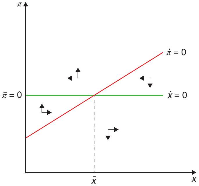
The graphical representation of this result is as follows. When drawn in \(\left[\pi_{t}, x_{t}\right]\) space, the Phillips curve is positively-sloped, while the IS schedule is horizontal, as you can see in the phase diagram in Figure 15.6. If \(x_{0}>\bar{x}\), there exists a \(\pi_{0}>\bar{\pi}\) such that both variables converge to the steady state in a south-westerly trajectory. The converse happens if \(x_{0}<\bar{x}\). Along a converging path, inflation and output do move together, as in the standard Phillips curve analysis. To see that, focus for instance on the south-west quadrant of the diagram. There, both output and inflation are below their long run levels, so that a depressed economy produces unusually low inflation. As output rises toward its longrun resting point, so does inflation.
But the important point is that there exists an infinity of such converging paths, one for each (arbitrary) initial condition! An exogenous path for the nominal interest, whichever path that may be, is not enough to pin down the rate of inflation (and the output gap) uniquely. What is the intuition for this indeterminacy or nonuniqueness? To see why self-fulfilling recessions may occur, suppose agents believe that output that is low today will gradually rise towards steady state. According to the NKPC, New Keynesian Phillips curve, a path of low output implies a path of low inflation. But with the nominal interest rate exogenously fixed, low expected inflation increases the real rate of interest and lowers consumption and output. The initial belief is thus self-fulfilling.
15.4.2 A Taylor rule in the canonical New Keynesian model
In Chapter 19 we further discuss interest rate policy and interest rate rules. Here we simply introduce the best-known and most-widely used rule: the Taylor rule, named after Stanford economist John
Taylor, who first proposed it as a description of the behaviour of monetary policy in the U.S. In Taylor (1993), the rule takes the form
\[ i_{t}=r_{t}^{n}+\phi_{\pi} \pi_{t}+\phi_{x} x_{t}, \tag{15.58}\]
where \(\phi_{\pi}\) and \(\phi_{x}\) are two coefficients chosen by the monetary authority. The choice of \(r_{t}^{n}\) requires it be equal to the normal or natural real rate of interest in the steady state. In what follows we will often assume \(\phi_{\pi}>1\), so that when \(\pi_{t}\) rises above the (implicit) target of 0, the nominal interest rises more than proportionately, and the real interest goes up in an effort to reduce inflation. Similarly, \(\phi_{x}>0\), so that when the output gap is positive, \(i_{t}\) rises from its normal level. Using the Taylor rule in the NKIS equation (15.42) yields
\[ \dot{x}_{t}=\sigma\left[\left(r_{t}^{n}-r^{n}\right)+\left(\phi_{\pi}-1\right) \pi_{t}+\phi_{x} x_{t}\right], \tag{15.59}\]
so that the rate of increase of the output gap is increasing in its own level and also increasing in inflation (because \(\phi_{\pi}-1>0\) ). The resulting dynamic system can be written as
\[ \left[\begin{array}{c} \dot{\pi} \\ \dot{x}_{\mathrm{t}} \end{array}\right]=\Omega\left[\begin{array}{c} \pi_{t} \\ x_{t} \end{array}\right]+\left[\begin{array}{c} 0 \\ \sigma\left(r_{t}^{n}-r^{n}\right) \end{array}\right] \tag{15.60}\]
where
\[ \Omega=\left[\begin{array}{cc} \rho & -\kappa \\ \sigma\left(\phi_{\pi}-1\right) & \sigma \phi_{x} \end{array}\right] . \tag{15.61}\]
Now \(\operatorname{Det}(\Omega)=\rho \sigma \phi_{x}+\sigma\left(\phi_{\pi}-1\right) \kappa>0\), and \(\operatorname{Tr}(\Omega)=\rho+\sigma \phi_{x}>0\). It follows that \(\phi_{\pi}>1\) is sufficient to ensure that both eigenvalues of \(\Omega\) are positive (or have positive real parts). Because both \(\pi_{\mathrm{t}}\) and \(x_{t}\) are jump variables, the steady state is now unique. After any permanent unanticipated shock, the system just jumps to the steady state and remains there!
As you can see in the phase diagram in Figure 15.7, the \(\dot{x}_{t}=0\) schedule (the NKIS) now slopes down. All four sets of arrows point away from the steady state point - which is exactly what you need to guarantee uniqueness of equilibrium in the case of a system of two jumpy variables!
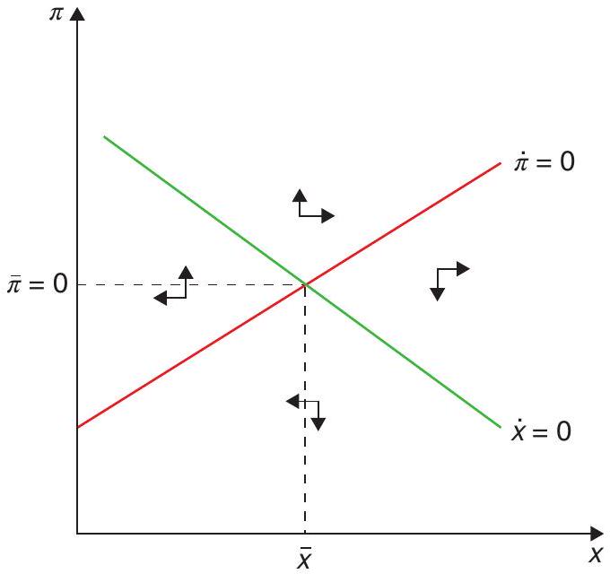
Go back to the expression \(\operatorname{Det}(\Omega)=\rho \phi_{x}+\sigma\left(\phi_{\pi}-1\right) \kappa\), which reveals that if \(\phi_{\pi}<1\) and \(\phi_{x}\) is not too large, then \(\operatorname{Det}(\Omega)<0\). Since, in addition, \(\operatorname{Tr}(\Omega)>0\), we would have a case of one positive and one negative eigenvalue, so that, again, multiplicity of equilibria (in fact, infinity of equilibria) would occur.
So there is an important policy lesson in all of this. In the canonical New Keynesian model, interest rate policy has to be sufficiently activist (aggressively anti-inflation, one might say), in order to guarantee uniqueness of equilibrium - in particular, to ensure that the rate of inflation and the output gap are pinned down. In the literature, policy rules where \(\phi_{\pi}>1\) are usually called active policy rules, and those where \(\phi_{\pi}<1\) are referred to as passive policy rules. Active policy rules are said to satisfy the ’Taylor principle’: sufficiently reactive interest rate policy pins down the equilibrium.
In this very simple model, which boils down to a system of linear differential equations, the uniqueness result is simple to derive and easy to understand. In more complex versions of the Keynesian model, -for instance, in non-linear models which need to be linearised around the steady state - or in circumstances in which the zero lower bound on the nominal interest rate binds, dynamics can be considerably more complicated, and the condition \(\phi_{\pi}>1\) in the Taylor rule need not be sufficient to guarantee uniqueness of equilibrium. For a more detailed treatment of these issues, see Benhabib et al. (2001a), Benhabib et al. (2001b), Benhabib et al. (2002), Woodford (2011), and Galí (2015).
Before ending this section, let us put this model to work by analysing a shock. Let’s imagine a monetary tightening implemented through a transitory exogenous increase in the interest rate (think of the interest moving to \(r_{t}^{n}+z\), with \(z\) the policy shifter), or, alternatively, imagine that at time 0, the natural rate of interest suddenly goes down from \(r^{n}\) to \(\underline{r}^{n}\), where \(0<\underline{r}^{n}<r^{n}\), because the trend rate of growth of output, \(g\), has temporarily dropped. After \(T>0\), either \(z\) goes back to zero, or the natural rate of interest goes back to \(r^{n}\) and remains there forever. How will inflation and output behave on impact, and in the time interval between times 0 and \(T\) ? The phase diagram in Figure 15.8 below shows the answer to these questions in a simple and intuitive manner.
Notice that either of these changes imply a leftward shift of the \(\dot{x}\) equation. So, during the transition the dynamics are driven by the original \(\dot{\pi}\) and new \(\dot{x}\) equations which intersect at point C.
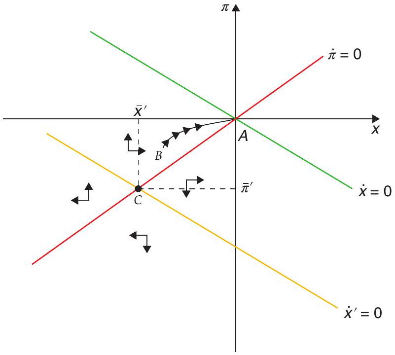
The system must return to A exactly at time \(T\). On impact, inflation and the output jump to a point, such as B, which is pinned down by the requirement that between 0 and \(T\) dynamics be those of the system with steady state at point C. That is, during the temporary shock the economy must travel to the north-east, with inflation rising and the output gap narrowing, in anticipation of the positive reversion of the shock at \(T\). Between 0 and \(T\) the negative shock, intuitively enough, causes output and inflation to be below their initial (and final, after \(T\) ) steady-state levels. If initially \(i^{n}=r^{n}\), so \(\bar{\pi}=0\) and \(\bar{x}=0\), as drawn below, then during the duration of the shock the economy experiences deflation and a recession (a negative output gap).11
What happens to the nominal interest rate? Between 0 and T, both inflation and the output gap are below their target levels of zero. So, the monetary authority relaxes the policy stance in response to both the lower inflation and the negative output gap. But that relaxation is not enough to keep the economy from going into recession and deflation. We return to this issue in Chapter 22.
15.4.3 Back to discrete time
The canonical New Keynesian model has a natural counterpart in discrete time, which is more broadly used for practical applications. In discrete time the Phillips curve becomes (see Galí (2015) for the detailed derivation)
\[ \pi_{\mathrm{t}}=\beta E_{\mathrm{t}} \pi_{t+1}+\kappa x_{t}, \tag{15.62}\]
where \(0<\beta=\frac{1}{1+\rho}<1\) is the discount factor, \(E_{t}\) is the expectations operator (with expectations computed as of time \(t\) ), and the output gap is again in logs. To derive the IS curve, again start from the Euler equation, which in logs can be written as
\[ y_{t}=E_{t} y_{t+1}-\sigma \log \left(1+r_{t}\right)+\sigma \log (1+\rho), \tag{15.63}\]
where we have already used \(c_{t}=y_{\mathrm{t}}\). If we recall the fact that for small \(r_{\mathrm{t}}\) and \(\rho, \log \left(1+r_{t}\right) \approx r_{t}\), and \(\log (1+\rho) \approx \rho\), equation (15.63) becomes
\[ y_{t}=E_{\mathrm{t}} y_{t+1}-\sigma\left(r_{\mathrm{t}}-\rho\right) . \tag{15.64}\]
Finally, subtracting \(\bar{y}\) from both sides yields
\[ x_{t}=E_{t} x_{t+1}-\sigma\left(i_{t}-E_{t} \pi_{t+1}-\rho\right), \tag{15.65}\]
where we have used the definition \(r_{t}=i_{t}-E_{t} \pi_{t+1}\) and the fact that \(x_{t}=y_{t}-\bar{y}\). If the natural rate of output is not constant, so that
\[ \bar{y}_{t+1}=\bar{y}_{t}+\Delta, \tag{15.66}\]
(15.65) becomes
\[ x_{t}=E_{\mathrm{t}} x_{t+1}+\Delta-\sigma\left(i_{t}-E_{\mathrm{t}} \pi_{t+1}-\rho\right) \tag{15.67}\]
or
\[ x_{t}=E_{t} x_{\mathrm{t}+1}-\sigma\left(i_{t}-E_{t} \pi_{\mathrm{t}+1}-r^{n}\right), \tag{15.68}\]
where
\[ r^{n}=\rho+\frac{\Delta}{\sigma}, \tag{15.69}\]
and again the variable \(r^{n}\) is the natural, or Wicksellian, interest rate, which can move around as a result of preference shocks (changes in \(\rho\) ) or productivity growth \((\Delta)\). To close the model, we can again appeal to an interest rule of the form
\[ i_{t}=i^{n}+\phi_{\pi} E_{t} \pi_{t+1}+\phi_{x} x_{t .} \tag{15.70}\]
As before, policy makers in charge of interest rate setting respond to deviations in expected inflation from the target (here equal to zero), and to deviations of output from the full employment or natural rate of output. Taylor argued that this rule (specifically, with \(\phi_{\pi}=1.5, \phi_{x}=0.5\) ), and an inflation target of \(2 \%\) is a good description of how monetary policy actually works in many countries - and, in particular, of how the Fed has behaved in modern times (since the mid-1980s).
There is an active research program in trying to compute optimal Taylor rules and also to estimate them from real-life data. In practice, no central bank has formally committed exactly to such a rule, but the analysis of monetary policy has converged onto some variant of a Taylor rule - and on interest rate rules more broadly - as the best way to describe how central banks operate.
Substituting the interest rate rule into the NKIS equation (15.70) (in the simple case of constant \(\bar{y}\) ) yields
\[ x_{\mathrm{t}}=E_{\mathrm{t}} x_{t+1}-\sigma\left[\left(\phi_{\pi}-1\right) E_{\mathrm{t}} \pi_{t+1}+\phi_{x} x_{\mathrm{t}}+\left(i^{n}-r^{n}\right)\right] . \tag{15.71}\]
This equation plus the NKPC constitute a system of two difference equations in two unknowns. As in the case of continuous time, it can be shown that an interest rule that keeps \(i_{t}\) constant does not guarantee uniqueness of equilibrium. But, it again turns out that if \(\phi_{\pi}>1\), a Taylor-type rule does ensure that both eigenvalues of the characteristic matrix of the \(2 \times 2\) system are larger than one. Since both \(\pi_{\mathrm{t}}\) and \(x_{t}\) are jumpy variables, that guarantees a unique outcome; the system simply jumps to the steady state and stays there.
To analyse formally the dynamic properties of this system, rewrite the NKPC (15.62) as
\[ E_{t} \pi_{t+1}=\beta^{-1} \pi_{t}-\beta^{-1} \kappa x_{t} . \tag{15.72}\]
Next, use this (15.71) to yield
\[ E_{t} x_{t+1}=\sigma\left(\phi_{\pi}-1\right) \beta^{-1} \pi_{t}+x_{t}+\sigma\left[-\left(\phi_{\pi}-1\right) \beta^{-1} \kappa+\phi_{x}\right] x_{t}+\sigma\left(i^{n}-r^{n}\right) . \tag{15.73}\]
(15.72) and (15.73) together constitute the canonical New Keynesian model in discrete time. In matrix form, the dynamic system is
\[ \left[\begin{array}{c} E_{t} \pi_{t+1} \\ E_{t} x_{t+1} \end{array}\right]=\Omega\left[\begin{array}{c} \pi_{t} \\ x_{t} \end{array}\right]+\left[\begin{array}{c} 0 \\ \sigma\left(i^{n}-r^{n}\right) \end{array}\right] \tag{15.74}\]
where
\[ \Omega=\left[\begin{array}{cc} \beta^{-1} & -\beta^{-1} \kappa \\ \sigma \beta^{-1}\left(\phi_{\pi}-1\right) & 1+\sigma\left[-\left(\phi_{\pi}-1\right) \beta^{-1} \kappa+\phi_{x}\right] \end{array}\right] . \tag{15.75}\]
Now
\[ \operatorname{Det}(\Omega)=\beta^{-1}\left(1+\sigma \phi_{x}\right)=\lambda_{1} \lambda_{2}>1 \tag{15.76}\]
and
\[ \operatorname{Tr}(\Omega)=\beta^{-1}+1+\sigma\left[\phi_{x}-\left(\phi_{\pi}-1\right) \beta^{-1} \kappa\right]=\lambda_{1}+\lambda_{2}, \tag{15.77}\]
where \(\lambda_{1}\) and \(\lambda_{1}\) are the eigenvalues of \(\Omega\). For both \(\lambda_{1}\) and \(\lambda_{2}\) to be larger than one, a necessary and sufficient condition is that
\[ \operatorname{Det}(\Omega)+1>\operatorname{Tr}(\Omega) \tag{15.78}\]
which, using the expressions for the determinant and the trace, is equivalent to
\[ \left(\phi_{\pi}-1\right) x+(1-\beta) \phi_{x}>0 . \tag{15.79}\]
This condition clearly obtains if \(\phi_{\pi}>1\). So, the policy implication is the same in both the continuous time and the discrete time of the model: an activist policy rule is required, in which the interest rate over-reacts to changes in the (expected) rate of inflation, in order to ensure uniqueness of equilibrium.
For a classic application of this model to monetary policy issues, see Clarida et al. (1999). In later chapters of this book we use the model to study a number of issues, some of which require the S to the DSGE acronym: shocks! As we saw in our discussion of RBC models, the business cycle properties we obtain from the model will depend on the properties we assume for those shocks.
The kind of DSGE model that is used in practice will add many bells and whistles to the canonical version, in the description of the behaviour of firms, households, and policy-makers. In doing so, it will open the door to a lot of different shocks as well. It will then try to either calibrate the model parameters, or estimate them using Bayesian techniques, and use the model to evaluate policy interventions. You will find in Appendix C a basic illustration of this kind of model, so you can do it for yourself!
These models will nevertheless keep the essential features of a firm grounding on household and firm optimisation, which is a way to address the Lucas Critique, and also of the consequent importance of expectations. We discuss the issues in greater detail in Chapter 17 and thereafter.
15.5 What have we learned?
We have gone over the basics of the Keynesian view of the business cycle, from its old IS-LM version to the modern canonical New Keynesian DSGE model. We saw the key role of imperfect price adjustment, leading to an upward-sloping aggregate supply curve, under which aggregate demand shocks have real consequences. We showed how imperfect competition and nominal (and real) rigidities are crucial for that. We saw how the Euler equation of consumption gives rise to the modern New Keynesian IS curve, while the Calvo model of price setting gives rise to the New Keynesian Phillips curve. Finally, we saw how we need to specify a policy rule (such as the Taylor rule) to close the model.
There is no consensus among macroeconomists as to whether the Keynesian or classical (RBC) view is correct. This is not surprising since they essentially involve very different world views in terms of the functioning of markets. Are market failures (at least relatively) pervasive, or can we safely leave them aside in our analysis? This is hardly the type of question that can be easily settled by the type of evidence we deal with in the social sciences.
Having said that, it’s important to stress the methodological convergence that has been achieved in macroeconomics, and that has hopefully been conveyed by our discussion in the last two chapters. Nowadays, essentially all of macro deals with microfounded models with rational agents, the difference being in the assumptions about the shocks and rigidities that are present (or absent) and driving the fluctuations. By providing a unified framework that allows policy makers to cater the model to what they believe are the constraints they face, means that the controversy about the fundamental discrepancies can be dealt, in a more flexible way within a unified framework. Imagine the issue of price rigidity, which is summarised by Calvo’s \(\alpha\) coefficient of price adjustment. If you believe in no price rigidities, \(\alpha\) has a specific value, if you think there are rigidities you just change the value. And nobody is going to fight for the value of \(\alpha\), are they? Worst case scenario, you just run it with both parameters and look at the output. No wonder then that the DSGE models have become a workhorse, for example, in Central Banking.
15.6 What next?
Any number of macro textbooks cover the basics of the Keynesian model, in its IS-LM version. The textbook by Romer (2018) covers the topics at the graduate level, and is a great introduction to the fundamentals behind the New Keynesian view. For the canonical, modern New Keynesian approach, the book by Galí (2015) is the key reference.
principles of laissez-faire to dig the notes up again (the right to do so being obtained, of course, by tendering for leases of the note-bearing territory), there need be no more unemployment and, with the help of the repercussions, the real income of the community, and its capital wealth also, would probably become a good deal greater than it actually is. It would, indeed, be more sensible to build houses and the like; but if there are political and practical difficulties in the way of this, the above would be better than nothing.”
References
Benhabib, J., Schmitt-Grohé, S., & Uribe, M. (2001a). Monetary policy and multiple equilibria. American Economic Review, 91(1), 167-186.
Benhabib, J., Schmitt-Grohé, S., & Uribe, M. (2001b). The perils of Taylor rules. Journal of Economic Theory, 96(1-2), 40-69.
Benhabib, J., Schmitt-Grohé, S., & Uribe, M. (2002). Avoiding liquidity traps. Journal of Political Economy, 110(3), 535-563.
Blanchard, O. & Galí, J. (2007). Real wage rigidities and the New Keynesian model. Journal of Money, Credit and Banking, 39, 35-65.
Calvo, G. A. (1983). Staggered prices in a utility-maximizing framework. Journal of Monetary Economics, 12(3), 383-398.
Clarida, R., Gali, J., & Gertler, M. (1999). The science of monetary policy: A New Keynesian perspective. Journal of Economic Literature, 37(4), 1661-1707.
Galí, J. (2015). Monetary policy, inflation, and the business cycle: An introduction to the New Keynesian framework and its applications. Princeton University Press.
Hicks, J. R. (1937). Mr. Keynes and the “classics”; A suggested interpretation. Econometrica, 147-159.
Lucas, R. E. (1973). Some international evidence on output-inflation tradeoffs. The American Economic Review, 63(3), 326-334.
Romer, D. (2018). Advanced macroeconomics. McGraw Hill.
Smets, F. & Wouters, R. (2003). An estimated dynamic stochastic general equilibrium model of the Euro area. Journal of the European Economic Association, 1(5), 1123-1175.
Taylor, J. B. (1993). Discretion versus policy rules in practice. Carnegie-Rochester Conference Series on Public Policy (Vol. 39, pp. 195-214). Elsevier.
Woodford, M. (2011). Interest and prices: Foundations of a theory of monetary policy. Princeton University Press.
Yun, T. (1996). Nominal price rigidity, money supply endogeneity, and business cycles. Journal of Monetary Economics, 37(2), 345-370.
This is what’s behind Keynes oft-quoted (and misquoted) statement (from Ch. 16 of the General Theory) that “To dig holes in the ground’, paid for out of savings, will increase, not only employment, but the real national dividend of useful goods and services.” (Note, however that he immediately goes on to say that ’it is not reasonable, however, that a sensible community should be content to remain dependent on such fortuitous and often wasteful mitigation when once we understand the influences upon which effective demand depends.’) Similarly, in Ch. 10 he states: “If the Treasury were to fill old bottles with banknotes, bury them at suitable depths in disused coalmines which are then filled up to the surface with town rubbish, and leave it to private enterprise on well-tried↩︎
As we will see, this is not exactly a Keynesian model; it was actually the opening shot in the rational expectations revolution. The New Keynesian approach, however, is the direct descendant of that revolution, by incorporating the rational expectations assumption and championing the role of aggregate demand policy under those conditions.↩︎
See Hicks (1937).↩︎
This is a simplifying assumption of certainty equivalence behaviour.↩︎
Note that this uses the law of iterated expectations, which states that \(E(E(p))=E(p)\) : you cannot be systematically wrong in your guess.↩︎
The mathematical intuition is as follows: because the firm is optimising in point A, the derivative of its income with respect to price is set at zero, and any gain from changing prices, from the firm’s perspective, will be of second order. But point A does not correspond to a social optimum, because of imperfect competition, and that means that the effects of a change in prices on social welfare will be of first order.↩︎
Somewhat confusingly, people often refer to the modern New Keynesian view of fluctuations and to DSGE models as synonyms. However, it is pretty obvious that RBC models are dynamic, stochastic, and general-equilibrium too! We prefer to keep the concepts separate, so we will always refer to New Keynesian DSGE models.↩︎
See Benhabib et al. (2001b), appendix B, for a full derivation in continuous time.↩︎
Implicit in this equation is the assumption that firms discount future profits at the household rate of discount.↩︎
Leibniz’s rule? Why, of course, you recall it from calculus: that’s how you differentiate an integral. If you need a refresher, here it is: take a function \(g(x)=\int_{a(x)}^{b(x)} f(x, s) d s\), the derivative of \(g\) with respect to \(x\) is: \(\frac{d g}{d x}=f(x, b(x)) \frac{d b}{d x}-f(x, a(x)) \frac{d a}{d x}+\int_{a(x)}^{b(x)} \frac{d f(x, s)}{d x} d s\). Intuitively, there are three components of the marginal impact of changing \(x\) on \(g\) : those of increasing the upper and lower limits of the integral (which are given by \(f\) evaluated at those limits), and that of changing the function \(f\) at every point between those limits (which is given by \(\int_{a(x)}^{b(x)} \frac{d f(x, s)}{d x} d s\) ). All the other stuff is what you get from your run-of-the-mill chain rule.↩︎
Whatever \(i^{n}\) was initially, in drawing the figure below we assume the intercept does not change in response to the shock – that is, it does not fall as the natural interest rate drops temporarily.↩︎