8 Overlapping generations models
The neoclassical growth model (NGM), with its infinitely-lived and identical individuals, is very useful for analysing a large number of topics in macroeconomics, as we have seen, and will continue to see, for the remainder of the book. However, there are some issues that require a departure from those assumptions. An obvious example involves those issues related to the understanding of the interaction of individuals who are at different stages in their life cycles. If lives are finite and not infinite, as in the NGM, individuals are not the same (or at a minimum are not at the same moment in their lives). This diversity opens a whole new set of issues, such as that of optimal consumption and investment over the life cycle, and the role of bequests. It also requires a redefinition of optimality. Not only because we need to address the issue of how to evaluate welfare when agents have different utility functions, but also because we will need to check if the optimality properties of the NGM prevail. For example, if there are poor instruments to save, yet people need to save for retirement, can it be possible that people accumulate too much capital?
This richer framework will provide new perspectives for evaluating policy decisions such as pensions, taxation, and discussing the impact of demographic changes. Of course, the analysis becomes more nuanced, but the added difficulty is not an excuse for not tackling the issue, particularly because in many instances the fact that individuals are different is the key aspect that requires attention.
To study these very important issues, in the next three chapters we develop the overlapping generations (OLG) model, the second workhorse framework of modern macroeconomics. We will see that, when bringing in some of these nuances, the implications of the model turn out to be very different from those of the NGM. This framework will also allow us to address many of the most relevant current policy debates in macroeconomics, including low interest rates, secular stagnation, and topics in fiscal and monetary policy.
8.1 The Samuelson-Diamond model
The Samuelson-Diamond model simplifies by assuming two generations: young and old. The young save for retirement, and this is the capital stock next period. The dynamics of capital will be summarised by a savings equation of the form \(s(w, r)\). This savings equation will allow us to trace the evolution of capital over time.
Here we present a discrete time model initially developed by Diamond (1965), building on earlier work by Samuelson (1958), in which individuals live for two periods (young and old). The economy lasts forever as new young people enter in every period. We first characterise the decentralised competitive equilibrium of the model. We then ask whether the market solution is the same as the allocation that would be chosen by a central planner, focusing on the significance of the golden rule, which will allow us to discuss the possibility of dynamic inefficiency (i.e. excessive capital accumulation).
8.1.1 The decentralized equilibrium
The market economy is composed of individuals and firms. Individuals live for two periods. They work for firms, receiving a wage. They also lend their savings to firms, receiving a rental rate.
An individual born at time \(t\) consumes \(c_{1 t}\) in period \(t\) and \(c_{2 t+1}\) in period \(t+1\), and derives utility
\[ \left(\frac{\sigma}{\sigma-1}\right) c_{1 t}^{\frac{\sigma-1}{\sigma}}+(1+\rho)^{-1}\left(\frac{\sigma}{\sigma-1}\right) c_{2 t+1}^{\frac{\sigma-1}{\sigma}}, \rho \geq 0, \sigma \geq 0 . \tag{8.1}\]
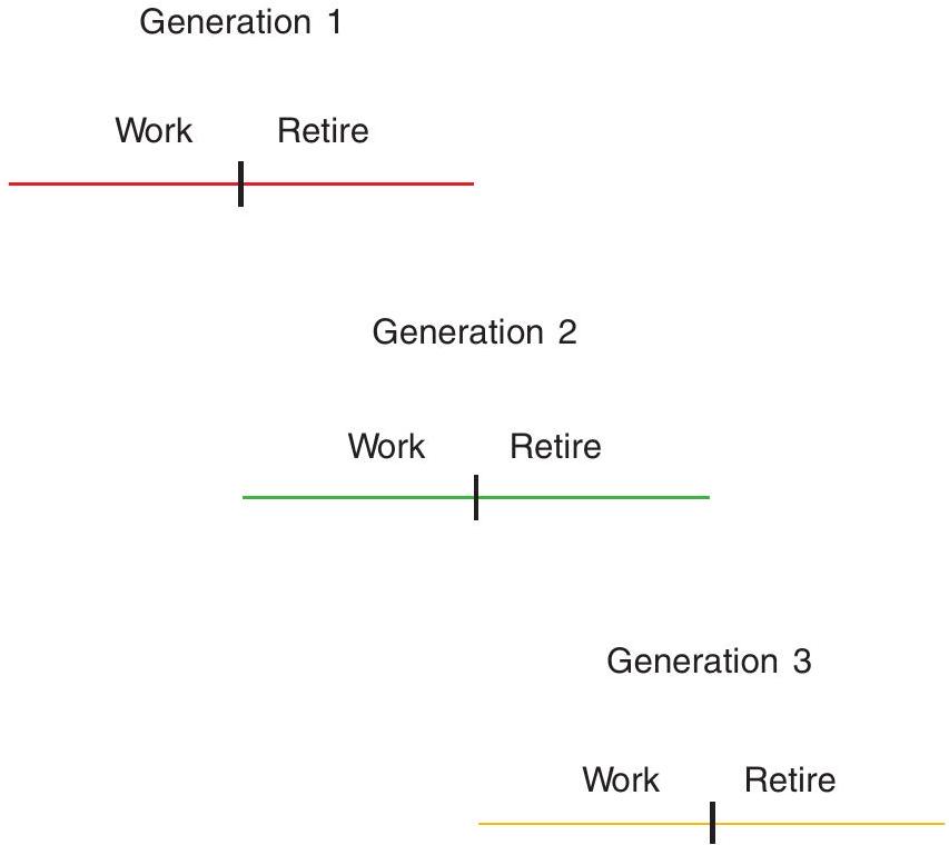
Note that the subscript “1” refers to consumption when young, and “2” labels consumption when old. Individuals work only in the first period of life, inelastically supplying one unit of labour and earning a real wage of \(w_{t}\). They consume part of their first-period income and save the rest to finance their second-period retirement consumption. The saving of the young in period \(t\) generates the capital stock that is used to produce output in period \(t+1\) in combination with the labour supplied by the young generation of period \(t+1\).
The time structure of the model appears in Figure 8.1.
The number of individuals born at time \(t\) and working in period \(t\) is \(L_{t}\). Population grows at rate \(n\) so that \(L_{t}=L_{0}(1+n)^{t}\).
Firms act competitively and use the constant returns technology \(Y=F(K, L)\). For simplicity, assume that capital fully depreciates after use, which is akin to assuming that \(F(\cdot, \cdot)\) is a net production function, with depreciation already accounted for. As before, output per worker, \(Y / L\), is given by the production function \(y=f(k)\), where \(k\) is the capital-labour ratio. This production function is assumed to satisfy the Inada conditions. Each firm maximises profits, taking the wage rate, \(w_{t}\), and the rental rate on capital, \(r_{t}\), as given.
We now examine the optimisation problem of individuals and firms and derive the market equilibrium.
Individuals
Consider an individual born at time \(t\). His maximisation problem is
\[ \operatorname{Max}\left\{\left(\frac{\sigma}{\sigma-1}\right) c_{1 t}^{\frac{\sigma-1}{\sigma}}+(1+\rho)^{-1}\left(\frac{\sigma}{\sigma-1}\right) c_{2 t+1}^{\frac{\sigma-1}{\sigma}}\right\} \tag{8.2}\]
subject to
\[ c_{1 t}+s_{t}=w_{t}, \tag{8.3}\]
\[ c_{2 t+1}=\left(1+r_{t+1}\right) s_{t}, \tag{8.4}\]
where \(w_{t}\) is the wage received in period \(t\) and \(r_{t+1}\) is the interest rate paid on savings held from period \(t\) to period \(t+1\). In the second period the individual consumes all his wealth, both interest and principal. (Note that this assumes that there is no altruism across generations, in that people do not care about leaving bequests to the coming generations. This is crucial.)
The first-order condition for a maximum is
\[ c_{1 t}^{-\frac{1}{\sigma}}-\left(\frac{1+r_{t+1}}{1+\rho}\right) c_{2 t+1}^{-\frac{1}{\sigma}}=0, \tag{8.5}\]
which can be rewritten as
\[ \frac{c_{2 t+1}}{c_{1 t}}=\left(\frac{1+r_{t+1}}{1+\rho}\right)^{\sigma} . \tag{8.6}\]
This is the Euler equation for the generation born at time \(t\). Note that this has the very same intuition, in discrete time, as the Euler equation (Ramsey rule) we derived in the context of the NGM.
Next, using (8.3) and (8.4) to substitute out for \(c_{1 t}\) and \(c_{2 t+1}\) and rearranging we get
\[ s_{t}=\left(\frac{1}{\left(1+r_{t+1}\right)^{1-\sigma}(1+\rho)^{\sigma}+1}\right) w_{t} . \tag{8.7}\]
We can think of this as a saving function:
\[ s_{t}=s\left(w_{t}, r_{t+1}\right), \quad 0<s_{w} \equiv \frac{\partial s_{t}}{\partial w_{t}}<1, s_{r} \equiv \frac{\partial s_{t}}{\partial r_{t+1}} \geq 0 \text { or } \leq 0 . \tag{8.8}\]
Saving is an increasing function of wage income since the assumption of separability and concavity of the utility function ensures that both goods (i.e. consumption in both periods) are normal. The effect of an increase in the interest rate is ambiguous, however, because of the standard income and substitution
effects with which you are familiar from micro theory. An increase in the interest rate decreases the relative price of second-period consumption, leading individuals to shift consumption from the first to the second period, that is, to substitute second- for first-period consumption. But it also increases the feasible consumption set, making it possible to increase consumption in both periods; this is the income effect. The net effect of these substitution and income effects is ambiguous. If the elasticity of substitution between consumption in both periods is greater than one, then in this two-period model the substitution effect dominates and an increase in interest rates leads to an increase in saving.
Firms
Firms act competitively, renting capital to the point where the marginal product of capital is equal to its rental rate, and hiring labour to the point where the marginal product of labour is equal to the wage
\[ f^{\prime}\left(k_{t}\right)=r_{t} \tag{8.9}\]
\[ f\left(k_{t}\right)-k_{t} f^{\prime}\left(k_{t}\right)=w_{t}, \tag{8.10}\]
where \(k_{t}\) is the firm’s capital-labour ratio. Note that \(f\left(k_{t}\right)-k_{t} f^{\prime}\left(k_{t}\right)\) is the marginal product of labour, because of constant returns to scale.
8.1.2 Goods and factor market equilibrium
The goods market equilibrium requires that the demand for goods in each period be equal to supply, or equivalently that investment be equal to saving:
\[ K_{t+1}-K_{t}=L_{t} s\left(w_{t}, r_{t+1}\right)-K_{t} . \tag{8.11}\]
The left-hand side is net investment: the change in the capital stock between \(t\) and \(t+1\). The right-hand side is net saving: the first term is the saving of the young; the second is the dissaving of the old.
Eliminating \(K_{t}\) from both sides tells us that capital at time \(t+1\) is equal to the saving of the young at time \(t\). Dividing both sides by \(L_{t}\) gives us the equation of motion of capital in per capita terms:
\[ (1+n) k_{t+1}=s\left(w_{t}, r_{t+1}\right) . \tag{8.12}\]
The services of labour are supplied inelastically; the supply of services of capital in period \(t\) is determined by the savings decision of the young made in period \(t-1\). Equilibrium in the factor markets obtains when the wage and the rental rate on capital are such that firms wish to use the available amounts of labour and capital services. The factor market equilibrium conditions are therefore given by equations (8.9) and (8.10).
8.1.3 The dynamics of the capital stock
The capital accumulation equation (8.12), together with the factor market equilibrium conditions (8.9) and (8.10), implies the dynamic behaviour of the capital stock:
\[ k_{t+1}=\frac{s\left[w\left(k_{t}\right), r\left(k_{t+1}\right)\right]}{1+n}, \tag{8.13}\]
or
\[ k_{t+1}=\frac{s\left[f\left(k_{t}\right)-k_{t} f^{\prime}\left(k_{t}\right), f^{\prime}\left(k_{t+1}\right)\right]}{1+n} . \tag{8.14}\]
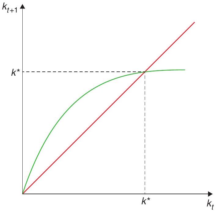
This last equation implies a relationship between \(k_{t+1}\) and \(k_{t}\). We will describe this as the savings locus. The properties of the savings locus depend on the derivative:
\[ \frac{d k_{t+1}}{d k_{t}}=\frac{-s_{w}\left(k_{t}\right) k_{t} f^{\prime \prime}\left(k_{t}\right)}{1+n-s_{r}\left(k_{t+1}\right) f^{\prime \prime}\left(k_{t+1}\right)} . \tag{8.15}\]
The numerator of this expression is positive, reflecting the fact that an increase in the capital stock in period \(t\) increases the wage, which increases savings. The denominator is of ambiguous sign because the effects of increases in the interest rate on savings are ambiguous. If \(s_{r} \geq 0\), then the denominator in (8.15) is positive, and then so is \(d k_{t+1} / d k_{t}\).
The savings locus in Figure 8.2 summarises both the dynamic and the steady-state behaviour of the economy. The 45-degree line in Figure 8.2 is the line along which steady states, at which \(k_{t+1}=k_{t}\), must lie. Any point at which the savings locus \(s\) crosses that line is a steady state. We have drawn a locus that crosses the 45-degree line only once, and hence guarantees that the steady state capital stock both exists and is unique. But this is not the only possible configuration. The model does not, without further restrictions on the utility and/or production functions, guarantee either existence or uniqueness of a steady-state equilibrium with positive capital stock.
If there exists a unique equilibrium with positive capital stock, will it be stable? To answer this, evaluate the derivative around the steady state:
\[ \left.\frac{d k_{t+1}}{d k_{t}}\right|_{S S}=\frac{-s_{w} k^{*} f^{\prime \prime}\left(k^{*}\right)}{1+n-s_{r} f^{\prime \prime}\left(k^{*}\right)} . \tag{8.16}\]
(Local) stability requires that \(\left.\frac{d k_{t+1}}{d k_{t}}\right|_{S S}\) be less than one in absolute value:
\[ \left|\frac{-s_{w} k^{*} f^{\prime \prime}\left(k^{*}\right)}{1+n-s_{r} f^{\prime \prime}\left(k^{*}\right)}\right|<1 . \]
Again, without further restrictions on the model, the stability condition may or may not be satisfied. To obtain definite results on the comparative dynamic and steady-state properties of the model, it is necessary either to specify functional forms for the underlying utility and production functions, or to impose conditions sufficient for uniqueness of a positive steady-state capital stock.1
8.1.4 A workable example
In this sub-section, we analyse the properties of the OLG model under a fairly simple set of assumptions: log utility (i.e. the limit case where \(\sigma=1\) ) and Cobb-Douglas production. (This is sometimes referred to as the canonical OLG model.) This permits a simple characterisation of both dynamics and the steady state.
With this assumption on preferences, the saving function is
\[ s_{t}=\left(\frac{1}{2+\rho}\right) w_{t}, \tag{8.17}\]
so that savings is proportional to wage income. Notice that the interest rate cancels out in the case of log utility, but not otherwise. This is a case in which the savings rate will be constant over time (as in the Solow model), though, once again, here this is the result of an optimal choice (as in the version of the AK model that we studied in Chapter 5).
With Cobb-Douglas technology, the firm’s rules for optimal behaviour (8.9) and (8.10) become
\[ r_{t}=\alpha k_{t}^{\alpha-1} \tag{8.18}\]
and
\[ w_{t}=(1-\alpha) k_{t}^{\alpha}=(1-\alpha) y_{t} . \tag{8.19}\]
Using (8.17) and (8.19) in (8.12) yields
\[ k_{t+1}=\left(\frac{1-\alpha}{2+\rho}\right)\left(\frac{1}{1+n}\right) k_{t}^{\alpha}, \tag{8.20}\]
which is the new law of motion for capital.
Define as usual the steady state as the situation in which \(k_{t+1}=k_{t}=k^{*}\). Equation (8.20) implies that the steady state is given by
\[ k^{*}=\left(\frac{1-\alpha}{2+\rho} \frac{1}{1+n}\right)^{\frac{1}{1-\alpha}}, \tag{8.21}\]
so that we have a unique and positive steady-state per-capita capital stock. This stock is decreasing in \(\rho\) (the rate of discount) and \(n\) (the rate of population growth). Note the similarities with the NGM and the Solow model.
Similarly, we can write steady-state income per-capita as \(y^{*}=\left(k^{*}\right)^{\alpha}\), or
\[ y^{*}=\left(\frac{1-\alpha}{2+\rho} \frac{1}{1+n}\right)^{\frac{\alpha}{1-\alpha}} . \tag{8.22}\]
Again, this steady-state level is decreasing in \(\rho\) and \(n\).
Will the system ever get to the steady state? Local stability requires that \(\left.\frac{d k_{t+1}}{d k_{t}}\right|_{S S}\) be less than one in absolute value, which in this case implies
\[ \alpha\left(\frac{1-\alpha}{2+\rho}\right)\left(\frac{1}{1+n}\right)\left(k^{*}\right)^{\alpha-1}=\alpha<1, \tag{8.23}\]
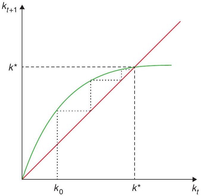
which is always satisfied. Hence, if the initial capital stock is larger than zero it will gradually converge to \(k^{*}\). Convergence is depicted in Figure 8.3. The economy starts out at \(k_{0}\) and gradually moves toward the steady-state capital stock.
The effects of a shock
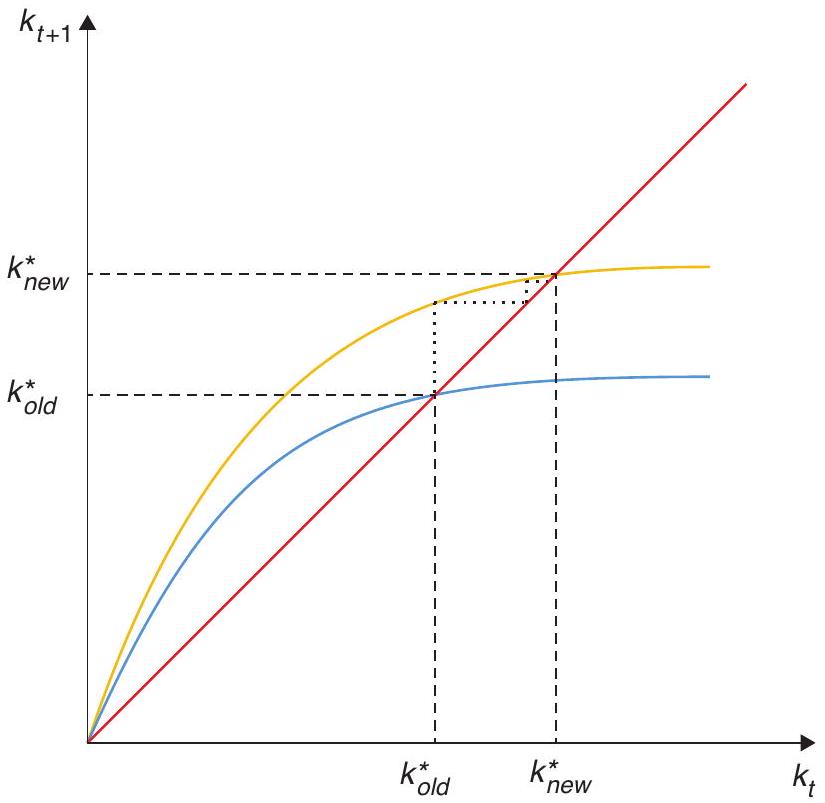
Suppose next that the economy is at the steady state and at some time 0 the discount rate falls from \(\rho\) to \(\rho^{\prime}\), where \(\rho^{\prime}<\rho\). This shock is unexpected, and will last forever.
From (8.21) we see that the new steady-state per capita capital stock will clearly rise, with \(k_{\text {new }}^{*}>\) \(k_{\text {old }}^{*}\). In Figure 8.4 we show the dynamic adjustment toward the new stationary position. The economy starts out at \(k_{\text {old }}^{*}\) and gradually moves toward \(k_{\text {new }}^{*}\). Income per capita rises in the transition and in the new steady state.
8.2 Optimality
The distinctive characteristic of the OLG model is that the interest rate may be smaller than the growth rate. In this case, there is a potential gain of reducing the stock of capital. The OLG model can lead to dynamic inefficiency.
We now ask how the market allocation compares to that which would be chosen by a central planner who maximises an intertemporal social welfare function. This raises a basic question, that of the relevant social welfare function. When individuals have infinite horizons and are all alike, it is logical to take the social welfare function to be their own utility function. But here the generations that are alive change as time passes, so it is not obvious what the central planner should maximise.
8.2.1 The steady-state marginal product of capital
In any event, as in the Solow model, there is something we can say about efficiency here. Notice that, at the steady state, the marginal product of capital is
\[ f^{\prime}\left(k^{*}\right)=\alpha\left(k^{*}\right)^{\alpha-1}=r^{*}=\left(\frac{\alpha}{1-\alpha}\right)(2+\rho)(1+n) . \tag{8.24}\]
Notice that this interest rate depends on more parameters than in the NGM. The relationship between the discount factor and the interest rate is still there. A higher discount factor implies less savings today and a higher interest rate in equilibrium. But notice that now that the population growth affects the interest rate. Why is this the case? The intuition is simple. A higher growth rate of population
decreases the steady-state stock of capital thus increasing the marginal product of capital. How does this compare with the golden rule of \(f^{\prime}\left(k_{G}\right)=n\) ? From the above it is clear that \(k^{*}>k_{G}\) if
\[ r^{*}<n, \tag{8.25}\]
which in turn implies
\[ \alpha<\frac{n}{n+(1+n)(2+\rho)} . \tag{8.26}\]
That is, if \(\alpha\) is sufficiently low (or, alternatively, if \(n\) is sufficiently high), the steady-state capital stock in the decentralised equilibrium can exceed that of the golden rule.
Dynamic inefficiency
Suppose a benevolent planner found that the economy was at the steady state with \(k^{*}\) and \(y^{*}\). Suppose further that \(k^{*}>k_{G}\). Is there anything the planner could do to redistribute consumption across generations that would make at least one generation better off without making any generation worse off? Put differently, is this steady state Pareto efficient?
Let resources available for per-capita consumption (of the young and old), in any period \(t\), be given by \(x_{t}\). Note next that in any steady state,
\[ x_{S S}=k_{S S}^{\alpha}-n k_{S S} . \tag{8.27}\]
Note that, by construction, \(k_{G}\) is the \(k_{S S}\) that maximises \(x_{S S}\), since \(\frac{\partial x_{S S}}{\partial k_{S S}}=0\).
The initial situation is one \(k_{S S}=k^{*}\), so that \(x_{S S}=c^{*}\). Suppose next that, at some point \(t=0\), the planner decides to allocate more to consumption and less to savings in that period, so that next period the capital stock is \(k_{G}<k^{*}\).
Then, in period 0 , resources available for consumption will be
\[ x_{0}=\left(k^{*}\right)^{\alpha}-n k_{G}+\left(k^{*}-k_{G}\right) . \tag{8.28}\]
In every subsequent period \(t>0\), resources available for consumption will be
\[ x_{t}=k_{G}^{\alpha}-n k_{G}, t>0 . \tag{8.29}\]
Clearly, in \(t>0\) available resources for consumption will be higher than in the status quo, since \(k_{G}\) maximises \(x_{S S}\). Note next that \(x_{0}>x_{t}\) (this should be obvious, since at time 0 those alive can consume the difference between \(k^{*}\) and \(k_{G}\) ). Therefore, in \(t=0\) resources available will also be higher than in the status quo. We conclude that the change increases available resources at all times. The planner can then split them between the two generations alive at any point in time, ensuring that everyone is at least as well off as in the original status quo, with at least one generation being better off. Put differently, the conclusion is that the decentralised solution leading to a steady state with a capital stock of \(k^{*}\) is not Pareto efficient. Generally, an economy with \(k^{*}>k_{G}\) (alternatively, one with \(r^{*}<n\) ) is known as a dynamically inefficient economy.
8.2.2 Why is there dynamic inefficiency?
If there is perfect competition with no externalities or other market failures, why is the competitive solution inefficient? Shouldn’t the First Welfare Theorem apply here as well? The reason why this isn’t the case is the infinity of agents involved, while the welfare theorems assume a finite number of agents.2
An alternative way to build this intuition is that when the interest rate is below the growth rate of the economy, budget constraints are infinite and not well-defined, making our economic restrictions meaningless. This infinity gives the planner a way of redistributing income and consumption across generations that is not available to the market. In a market economy, individuals wanting to consume in old age must hold capital, even if the marginal return on capital is low. The planner, by contrast, can allocate resources between the current old and young in any manner they desire. They can take part of the fruit of the labour income of the young, for instance, and transfer it to the old without forcing them to carry so much capital. They can make sure that no generation is worse off by requiring each succeeding generation to do the same (and remember, there are infinitely many of them).3 And, if the marginal product of capital is sufficiently low (lower than \(n\), so the capital stock is above the golden rule), this way of transferring resources between young and old is more efficient than saving, so the planner can do better than the decentralized allocation.
8.2.3 Are actual economies dynamically inefficient?
Recall that in the decentralised equilibrium we had
\[ r_{S S}=f^{\prime}\left(k_{S S}\right), \tag{8.30}\]
so the rental rate is equal to the marginal product of capital. Notice also that the rate of growth of the economy is \(n\) (income per-capita is constant, and the number of people is growing at the rate \(n\) ). Therefore, the condition for dynamic inefficiency is simply that \(r_{S S}\) be lower than the rate of growth of the economy, or, taking depreciation into account (which we have ignored here), that the rate of interest minus depreciation be lower than the rate of growth of the economy.
Abel et al. (1989) extend the model to a context with uncertainty (meaning that there is more than one observed interest rate, since you have to adjust for risk), and show that in this case a sufficient condition for dynamic efficiency is that net capital income exceeds investment. To understand why, notice that the condition for dynamic efficiency is that the marginal product of capital \((r)\) exceeds the growth rate of population \((n)\), which happens to be the growth rate of the economy \(g\). So, \(r K\) is the total return to capital and \(n K\) is total investment, so the condition \(r>g\) can be tested by comparing the return on capital vs new investment: the net flow out of firms. Their evidence from seven industrialised countries suggests that this condition seems to be comfortably satisfied in practice.
However, a more recent appraisal, by Geerolf (2013), suggests that this picture may have actually changed or never been quite as sanguine. He updates the Abel et al. data, and provides a different treatment to mixed income and land rents.4 With these adjustments, he finds that, in general, countries are in dynamically efficient positions, though some countries such as Japan and South Korea are definitely in a dynamically inefficient state! (And Australia joins the pack more recently…) In other words, it seems at the very least that we cannot so promptly dismiss dynamic inefficiency as a theoretical curiosity.
8.2.4 Why is this important?
At this point you may be scratching your head asking why we seem to be spending so much time with the question of dynamic efficiency. The reason is that it is actually very relevant for a number of issues. For example, a dynamically inefficient economy is one in which fiscal policy has more leeway. Any debt level will eventually be wiped out by growth. Blanchard (2019) (p. 1197) takes this point seriously and argues
… the current U.S. situation, in which safe interest rates are expected to remain below growth rates for a long time, is more the historical norm than the exception. If the future is like the past, this implies that debt rollovers, that is the issuance of debt without a later increase in taxes, may well be feasible. Put bluntly, public debt may have no fiscal cost.
Not surprisingly, during 2020/2021, in response to the Covid-19 pandemic, many countries behaved as if they could tap unlimited resources through debt issuing. Dynamic inefficiency, if present and expected to remain in the future, would say that was feasible. If, on the contrary, economies are dynamically efficient, the increases in debt will require more taxes down the road.
The second issue has to do with the possibility of bubbles, that is, assets with no intrinsic value. By arbitrage, the asset price of a bubble will need to follow a typical pricing equation
\[ (1+r) P_{t}=P_{t+1}, \tag{8.31}\]
assuming for simplification a constant interest rate. The solution to this equation is
\[ P_{t}=P_{0}(1+r)^{t}, \tag{8.32}\]
(simply replace to check it is a solution). The price of the asset needs to grow at the rate of interest rate (you may hold a dividend-less asset, but you need to get your return!). In an NGM where \(r>g\), this asset cannot exist, because it will eventually grow to become larger than the economy. But if \(r<g\) this is not the case, and the bubble can exist. We will come back to this later. What are examples of such assets? Well, you may have heard about Bitcoins and cryptocurrency. In fact, money itself is really a bubble!
Finally, notice that the OLG model can deliver very low interest rates. So, it is an appropriate setup to explain the current world of low interest rates. We will come back to this in our chapters on fiscal and monetary policy.
Before this, however, we need to provide a continuous-time version of the OLG model, to provide continuity with the framework we have been using so far, and because it will be useful later on.
8.3 Overlapping generations in continuous time
The OLG model can be modelled in continuous time through an ingenious mechanism: a constant probability of death and the possibility of pre-selling your assets upon death in exchange for a payment while you live. This provides cohorts and steady-state behaviour that make the model tractable. Even so, the details get a bit eerie. This section is only for the brave-hearted.
The trick to model the OLG model in a continuous-time framework is to include an age-independent probability of dying \(p\). By the law of large numbers this will also be the death rate in the population. Assume a birth rate \(n>p\). Together these two assumptions imply that population grows at the rate \(n-p\).5 This assumption is tractable but captures the spirit of the OLG model: not everybody is the same at the same time.
As in Blanchard (1985), we assume there exist companies that allow agents to insure against the risk of death (and, therefore, of leaving behind unwanted bequests). This means that at the time of death all of an individual’s assets are turned over to the insurance company, which in turn pays a return of \(p\) on savings to all agents who remain alive. If \(r_{t}\) is the interest rate, then from the point of view of an individual agent, the return on savings is \(r_{t}+p\).
We will also assume logarithmic utility which will make the algebra easier. As of time \(t\) the representative agent of the generation born at time \(\tau\) maximises
\[ \int_{t}^{\infty} \log c_{s, \tau} e^{-(\rho+p)(s-t)} d s \tag{8.33}\]
subject to the flow budget constraint
\[ \dot{a}_{t, \tau}=\left(r_{t}+p\right) a_{t, \tau}+y_{t, \tau}-c_{t, \tau}, \tag{8.34}\]
where \(a_{t, \tau}\) is the stock of assets held by the individual and \(y_{t, \tau}\) is labour income. The other constraint is the no-Ponzi game condition requiring that if the agent is still alive at time \(s\), then
\[ \lim _{s \rightarrow \infty} a_{s, \tau} e^{-\int_{t}^{s}\left(r_{v}+p\right) d v} \geq 0 \tag{8.35}\]
If we integrate the first constraint forward (look at our Mathematical Appedix!) and use the second constraint, we obtain
\[ \int_{t}^{\infty} c_{s, \tau} e^{-\int_{t}^{s}\left(r_{v}+p\right) d v} d s \leq a_{t, \tau}+h_{t, \tau} \tag{8.36}\]
where
\[ h_{t, \tau}=\int_{t}^{\infty} y_{s, \tau} e^{-\int_{t}^{s}\left(r_{v}+p\right) d v} d s, \tag{8.37}\]
can be thought of as human capital. So the present value of consumption cannot exceed available assets, a constraint that will always hold with equality.
With log utility the individual Euler equation is our familiar
\[ \dot{c}_{s, \tau}=\left(r_{s}-\rho\right) c_{s, \tau}, \tag{8.38}\]
which can be integrated forward to yield
\[ c_{s, \tau}=c_{t, \tau} e^{\int_{t}^{s}\left(r_{v}-\rho\right) d v} . \tag{8.39}\]
Using this in the present-value budget constraint gives us the individual consumption function
\[ \begin{gathered} \int_{t}^{\infty} c_{t, \tau} \int_{t}^{s}\left(r_{v}-\rho\right) d v e^{-\int_{t}^{s}\left(r_{v}+p\right) d v} d s=a_{t, \tau}+h_{t, \tau} \\ c_{t, \tau} \int_{t}^{\infty} e^{-(\rho+p)(s-t)} d s=a_{t, \tau}+h_{t, \tau}\\ c_{t, \tau}=(\rho+p)\left(a_{t, \tau}+h_{t, \tau}\right) \end{gathered} \tag{8.40}\]
so that the individual consumes a fixed share of available assets, as is standard under log utility. That completes the description of the behaviour of the representative agent in each generation.
The next task is to aggregate across generations or cohorts. Let \(N_{t, \tau}\) be the size at time \(t\) of the cohort born at \(\tau\). Denoting the total size of the population alive at time \(\tau\) as \(N_{\tau}\), we can write the initial size of the cohort born at \(\tau\) (that is, the newcomers to the world at \(\tau\) ) as \(n N_{\tau}\). In addition, the probability that someone born at \(\tau\) is still alive at \(t \geq \tau\) is \(e^{-p(t-\tau)}\). It follows that
\[ N_{t, \tau}=n N_{\tau} e^{-p(t-\tau)} . \tag{8.41}\]
Now taking into account deaths and births, we can write the size of the total population alive at time \(t\) as a function of the size of the population that was alive at some time \(\tau\) in the past: \(N_{t}=N_{\tau} e^{(n-p)(t-\tau)}\). It follows that
\[ \frac{N_{t, \tau}}{N_{t}}=n e^{-p(t-\tau)} e^{-(n-p)(t-\tau)}=n e^{-n(t-\tau)} . \tag{8.42}\]
We conclude that the relative size at time \(t\) of the cohort born at \(\tau\) is simply \(n e^{-n(t-\tau)}\).
For any variable \(x_{t, \tau}\) define the per capita (or average) \(x_{t}\) as
\[ \begin{aligned} & x_{t}=\int_{-\infty}^{t} x_{t, \tau}\left(\frac{N_{t, \tau}}{N_{t}}\right) d \tau\\ & x_{t}=\int_{-\infty}^{t} x_{t, \tau} n e^{-n(t-\tau)} d \tau \end{aligned} \tag{8.43}\]
Applying this definition to individual consumption from (8.40) we have
\[ c_{t}=(\rho+p)\left(a_{t}+h_{t}\right), \tag{8.44}\]
so that per capita consumption is proportional to per capita assets, where
\[ a_{t}=\int_{-\infty}^{t} a_{t, \tau} n e^{-n(t-\tau)} d \tau, \tag{8.45}\]
and
\[ h_{t}=\int_{-\infty}^{t} h_{t, \tau} n e^{-n(t-\tau)} d \tau, \tag{8.46}\]
are non-human and human wealth, respectively. Focus on each, beginning with human wealth, which using the expression for \(h_{t, \tau}\) in (8.37) can be written as
\[ h_{t}=\int_{-\infty}^{t}\left\{\int_{t}^{\infty} y_{s, \tau} e^{-\int_{t}^{s}\left(r_{v}+p\right) d v} d s\right\} n e^{-n(t-\tau)} d \tau . \tag{8.47}\]
Now, if labour income is the same for all agents who are alive at some time \(s\), we have
\[ h_{t}=\int_{-\infty}^{t}\left\{\int_{t}^{\infty} y_{s} e^{-\int_{t}^{s}\left(r_{v}+p\right) d v} d s\right\} n e^{-n(t-\tau)} d \tau, \tag{8.48}\]
where the expression in curly brackets is the same for all agents. It follows that
\[ h_{t}=\int_{t}^{\infty} y_{s} e^{-\int_{t}^{s}\left(r_{v}+p\right) d v} d s \tag{8.49}\]
Finally, differentiating with respect to time \(t\) (with the help of Leibniz’s rule) we arrive at6
\[ \dot{h}_{t}=\left(r_{t}+p\right) h_{t}-y_{t}, \tag{8.50}\]
which is the equation of motion for human capital. It can also we written as
\[ r_{t}+p=\frac{\dot{h}_{t}+y_{t}}{h_{t}} . \tag{8.51}\]
This has our familiar, intuitive asset pricing interpretation. If we think of human capital as an asset, then the RHS is the return on this asset, including the capital gain \(\dot{h}_{t}\) and the dividend \(y_{t}\), both
expressed in proportion to the value \(h_{t}\) of the asset. That has to be equal to the individual discount rate \(r_{t}+p\), which appears on the LHS.
Turn next to the evolution of non-human wealth. Differentiating \(a_{t}\), from (8.45), with respect to \(t\) (again using Leibniz’s rule!) we have
\[ \begin{gathered} \dot{a}_{t}=n a_{t}+n \int_{-\infty}^{t}\left\{-a_{t, \tau} n e^{-n(t-\tau)}+e^{-n(t-\tau)} \dot{a}_{t, \tau}\right\} d \tau,\\ \dot{a}_{t}=n a_{t, 0}-n a_{t}+n \int_{-\infty}^{t} \dot{a}_{t, \tau} e^{-n(t-\tau)} d \tau, \end{gathered} \tag{8.52}\]
since \(a_{t, 0}\) is non-human wealth at birth, which is zero for all cohorts, we have
\[ \begin{gathered} \dot{a}_{t}=-n a_{t}-n \int_{-\infty}^{t} \dot{a}_{t, \tau} e^{-n(t-\tau)} d \tau, \\ \dot{a}_{t}=-n a_{t}+\int_{-\infty}^{t}\left\{\left(r_{t}+p\right) a_{t, \tau}+y_{t}-c_{t, \tau}\right\} n e^{-n(t-\tau)} d \tau, \\ \dot{a}_{t}=-n a_{t}+\left(r_{t}+p\right) \int_{-\infty}^{t} a_{t, \tau} n e^{-n(t-\tau)} d \tau+y_{t} \int_{-\infty}^{t} n e^{-n(t-\tau)} d \tau-\int_{-\infty}^{t} c_{t, \tau} n e^{-n(t-\tau)} d \tau,\\ \dot{a}_{t}=\left[r_{t}-(n-p)\right] a_{t}+y_{t}-c_{t} . \end{gathered} \tag{8.53}\]
Notice that while the individual the rate of return is \(r_{t}+p\), for the economy as a whole the rate of return is only \(r_{t}\), since the \(p\) is a transfer from people who die to those who remain alive, and washes out once we aggregate. Recall, however, that \(a_{t}\) is assets per capita, so naturally \((n-p)\), the rate of growth of population, must be subtracted from \(r_{t}\).
The consumption function (8.40) and the laws of motion for per capita human and non-human wealth, (8.50) and (8.53), completely characterise the dynamic evolution of this economy. It can be expressed as a two-dimensional system in the following way. Differentiate the consumption function with respect to time in order to obtain
\[ \dot{c}_{t}=(\rho+p)\left(\dot{a}_{t}+\dot{h}_{t}\right) . \tag{8.54}\]
Next use the laws of motion for both forms of wealth to obtain
\[ \dot{c}_{t}=(\rho+p)\left[\left(r_{t}-n+p\right) a_{t}-c_{t}+\left(r_{t}+p\right) h_{t}\right] . \tag{8.55}\]
Write the consumption function in the following way
\[ h_{t}=\frac{c_{t}}{\rho+p}-a_{t}, \tag{8.56}\]
and use it to substitute out \(h_{t}\) from the \(\dot{c}_{t}\) equation (8.55):
\[ \begin{gathered} \dot{c}_{t}=(\rho+p)\left[\left(r_{t}-n+p\right) a_{t}-c_{t}-\left(r_{t}+p\right) a_{t}+\frac{r_{t}+p}{\rho+p} c_{t}\right], \\ \dot{c}_{t}=(\rho+p)\left[-n a_{t}+\frac{r_{t}-\rho}{\rho+p} c_{t}\right],\\ \dot{c}_{t}=\left(r_{t}-\rho\right) c_{t}-n(p+\rho) a_{t} . \end{gathered} \tag{8.57}\]
This is a kind of modified Euler equation. The first term is standard, of course, but the second term is not. That second term comes from the fact that, at any instant, there are \(n\) newcomers for each person alive, and they dilute assets per capita by \(n a_{t}\) since at birth they have no assets. This slows down the average rate of consumption growth.
This modified Euler equation plus the law of motion for non-human wealth (8.53) are a two-dimensional system of differential equations in \(c_{t}\) and \(a_{t}\). That system, plus an initial condition and a transversality condition for \(a_{t}\), fully describes the behaviour of the economy.
8.3.1 The closed economy
We have not taken a stance on what kind of asset \(a_{t}\) is. We now do so. In the closed economy we assume that \(a_{t}=k_{t}\), and \(k_{t}\) is per-capita productive capital that yields output according to the function \(y_{t}=k_{t}^{\alpha}\), where \(0<\alpha<1\). In this context profit maximisation dictates that \(r_{t}=\alpha k_{t}^{\alpha-1}\), so that our two differential equations become
\[ \begin{aligned} & \dot{c}_{t}=\left(\alpha k_{t}^{\alpha-1}-\rho\right) c_{t}-n(p+\rho) k_{t}, \\ & \dot{k}_{t}=(1+\alpha) k_{t}^{\alpha}-(n-p) k_{t}-c_{t} . \end{aligned} \tag{8.58}\]
In steady state we have
\[ \begin{gathered} \frac{c^{*}}{k^{*}}=\frac{n(p+\rho)}{\alpha k^{* \alpha-1}-\rho},\\ (1+\alpha) k^{* \alpha-1}-(n-p)=\frac{c^{*}}{k^{*}} . \end{gathered} \tag{8.59}\]
Combining the two yields
\[ (1+\alpha) k^{* \alpha-1}=(n-p)+\frac{n(p+\rho)}{\alpha k^{* \alpha-1-\rho}}, \tag{8.60}\]
which pins down the capital stock. For given \(k^{*}\), the first SS equation yields consumption. Rewrite the last equation as
\[ \alpha k^{* \alpha-1}-\rho=\frac{n(p+\rho)}{(1+\alpha) k^{* \alpha-1}-(n-p)}>0 . \tag{8.61}\]
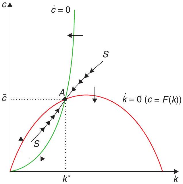
So the steady-state level of the (per capita) capital stock is smaller than the modified golden rule level that solves \(\alpha k^{\alpha-1}=\rho\), implying under-accumulation of capital.7 This is in contrast to the NGM, in which the modified golden rule applies, and the discrete-time OLG model with two-period lives, in which over-accumulation may occur. Before examining that issue, consider dynamics, described in Figure 8.5.
Along the saddle-path \(c_{t}\) and \(k_{t}\) move together. If the initial condition is at \(k>k^{*}\), then consumption will start above its SS level and both \(c_{t}\) and \(k_{t}\) will gradually fall until reaching the steady-state level. If, by contrast, the initial condition is at \(k<k^{*}\), then consumption will start below its steadystate level and both \(c_{t}\) and \(k_{t}\) will rise gradually until reaching the steady state.
8.3.2 A simple extension
But how come we have no dynamic inefficiency in this model? Just switching to continuous time does away with this crucial result? Not really. The actual reason is that the model so far is not quite like what we had before, in another aspect: there is no retirement! In contrast to the standard OLG model, individuals have a smooth stream of labour income throughout their lives, and hence do not need to save a great deal in order to provide for consumption later in life.
Introducing retirement (i.e. a stretch of time with no income, late in life) is analytically cumbersome, but as Blanchard (1985) demonstrates, there is an alternative that is easily modelled, has the same flavour, and delivers the same effects: assuming labour income declines gradually as long as an individual is alive.
Let’s take a look. Blanchard (1985) assumes that each individual starts out with one unit of effective labour and thereafter his available labour declines at the rate \(\gamma>0\). At time \(t\), the labour earnings of a person in the cohort born at \(\tau\) is given by \(w_{t} e^{-\gamma(t-\tau)}\), where \(w_{t}\) is the market wage per unit of effective labour at time \(t\). It follows that individual human wealth for a member of the \(\tau\) generation is
\[ h_{t, \tau}=\int_{t}^{\infty} w_{s} e^{-\gamma(s-\tau)} e^{-\int_{t}^{s}\left(r_{v}+p\right) d v} d s \tag{8.62}\]
Using the same derivation as in the baseline model, we arrive at a modified Euler equation
\[ \dot{c}_{t}=\left(\alpha k_{t}^{\alpha-1}+\gamma-\rho\right) c_{t}-(n+\gamma)(p+\rho) k_{t}, \tag{8.63}\]
which now includes the parameter \(\gamma\).
The steady state per-capita capital stock is now again pinned down by the expression
\[ k^{* \alpha-1}=(n-p)+\frac{(n+\gamma)(p+\rho)}{\alpha+\gamma-\rho}, \tag{8.64}\]
which can be rewritten as
\[ \alpha k^{* \alpha-1}-\rho=\frac{(n+\gamma)(p+\rho)}{k^{* \alpha-1}-(n-p)}-\gamma . \tag{8.65}\]
So if \(\gamma\) is sufficiently large, then the steady-state per capita capital stock can be larger than the golden rule level, which is the one that solves the equation \(\alpha k^{\alpha-1}=\rho\). This would imply over-accumulation of capital. The intuition is that the declining path of labour income forces people to save more, too much in fact. Again, intergenerational transfers would have been a more efficient way to pay for retirement, but they cannot happen in the decentralized equilibrium, in the absence of intergenerational altruism.
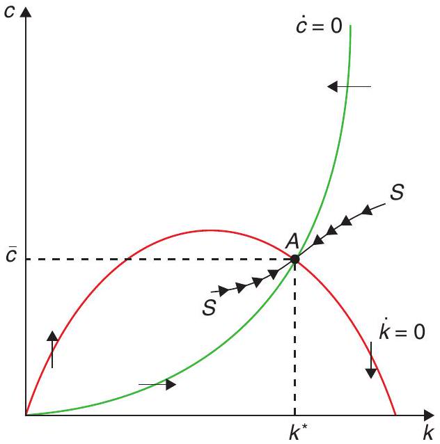
In this case, dynamics are given by Figure 8.6, with the steady state to the right of the modified golden-rule level of capital:
8.3.3 Revisiting the current account in the open economy
We can also revisit the small open economy as a special case of interest. For that, let’s go back to the case in which \(\gamma=0\), and consider what happens when the economy is open, and instead of being capital, the asset is a foreign bond \(f_{t}\) that pays the fixed world interest rate \(r\). In turn, labour income is now, for simplicity, an exogenous endowment \(y_{t, \tau}=y\) for all moments \(t\) and for all cohorts \(\tau\).
The two key differential equations now become
\[ \begin{aligned} & \dot{c}_{t}=(r-\rho) c_{t}-n(p+\rho) f_{t}, \\ & \dot{f}_{t}=[r-(n-p)] f_{t}+y-c_{t}, \end{aligned} \tag{8.66}\]
with steady-state values
\[ [r-(n-p)] f^{*}+y=c^{*}, \tag{8.67}\]
\[ (r-\rho) c^{*}=n(p+\rho) f^{*}, \tag{8.68}\]
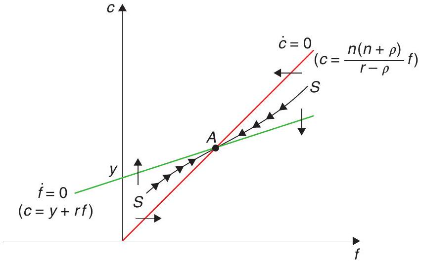
which together pin down the levels of consumption and foreign assets. The first equation reveals that in steady state the current account must be balanced, with consumption equal to endowment income plus interest earnings from foreign assets. As the second equation reveals, the steady-state stock of foreign assets can be positive or negative, depending on whether \(r\) is larger or smaller than \(\rho\).
If \(r>\rho\), individual consumption is always increasing, agents are accumulating over their lifetimes, and the steady-state level of foreign assets is positive. If \(r=\rho\), individual consumption is flat and they neither save nor dissave; steady-state foreign assets are zero. Finally, if \(r<\rho\), individual consumption is always falling, agents are decumulating over their lifetimes, and in the steady state the economy is a net debtor.
Equilibrium dynamics are given by Figure 8.7, drawn for the case \(r>\rho\). It is easy to show that the system is saddle-path stable if \(r<\rho+p\). So the diagram below corresponds to the case \(\rho<r<\rho+p\). Along the saddle-path, the variables \(c_{t}\) and \(f_{t}\) move together until reaching the steady state.
In this model the economy does not jump to the steady state (as the open-economy model in Chapter 4 did). The difference is that new generations are constantly being born without any foreign assets and they need to accumulate them. The steady state is reached when the accumulation of the young offsets the decumulation of the older generation.
8.4 What have we learned?
In this chapter we developed the second workhorse model of modern macroeconomics: the OLG model. This framework allows us to look at questions in which assuming a single representative agent is not a useful shortcut. We will see how this will enable us to tackle some key policy issues, starting in the next chapter.
Moreover, we have already shown how this model yields new insights about capital accumulation, relative to the NGM. For instance, the possibility of dynamic inefficiency - that is to say, of over-accumulation of capital - emerges. This is a result of the absence of intergenerational links, which entail that individuals may need to save too much, as it is the only way to meet their consumption needs as their labor income declines over their life cycle.
Notes
References
Abel, A. B., Mankiw, N. G., Summers, L. H., & Zeckhauser, R. J. (1989). Assessing dynamic efficiency: Theory and evidence. The Review of Economic Studies, 56(1), 1-19.
Blanchard, O. (2019). Public debt and low interest rates. American Economic Review, 109(4), 1197-1229.
Blanchard, O. J. (1985). Debt, deficits, and finite horizons. Journal of Political Economy, 93(2), 223-247.
Diamond, P. A. (1965). National debt in a neoclassical growth model. The American Economic Review, 55(5), 1126-1150.
Geerolf, F. (2013). Reassessing dynamic efficiency. Manuscript, Toulouse School of Economics.
Samuelson, P. A. (1958). An exact consumption-loan model of interest with or without the social contrivance of money. Journal of Political Economy, 66(6), 467-482.
If the production function makes the function hit the 45-degree line with a negative slope the model can give origin to cyclical behaviour around the steady-state. This cycle can be stable or unstable depending on the slope of the curve.↩︎
The First Welfare Theorem can be extended to deal with an infinite number of agents, but this requires a condition that the total value of resources available to all agents taken together be finite (at equilibrium prices). This is not satisfied in the OLG economy, which lasts forever.↩︎
For those of you who are mathematically inclined, the argument is similar to Hilbert’s Grand Hotel paradox. If the argument sounds counter-intuitive and esoteric, it’s because it is - so much so that some people apparently think the paradox can be used to prove the existence of God! (see http: //en.wikipedia.org/wiki/Hilbert’s_paradox_of_the_Grand_Hotel).↩︎
Mixed income is that which is registered as accruing to capital, because it comes from the residual income of businesses, but that Geerolf argues should be better understood, at least partly as, returns to entrepreneurial labour. Land rents, which Abel et al. only had for the U.S., should not be understood as capital in their sense, as land cannot be accumulated.↩︎
Suppose, in addition, that the economy starts with a population \(N_{0}=1\).↩︎
Leibniz’s rule? Why, of course, you recall it from calculus: that’s how you differentiate an integral. If you need a refresher, here it is: take a function \(g(x)=\int_{a(x)}^{b(x)} f(x, s) d s\), the derivative of \(g\) with respect to \(x\) is: \(\frac{d g}{d x}=f(x, b(x)) \frac{d b}{d x}-f(x, a(x)) \frac{d a}{d x}+\int_{a(x)}^{b(x)} \frac{d f(x, s)}{d x} d s\). Intuitively, there are three components of the marginal impact of changing \(x\) on \(g\) : those of increasing the upper and lower limits of the integral (which are given by \(f\) evaluated at those limits), and that of changing the function \(f\) at every point between those limits (which is given by \(\int_{a(x)}^{b(x)} \frac{d f(x, s)}{d x} d s\) ). All the other stuff is what you get from your run-of-the-mill chain rule.↩︎
Because individuals discount the future \((\rho>0)\), this is not the same as the golden rule in the Solow model, which maximises consumption on the steady state. In the modified golden rule, the capital stock is smaller than that which maximises consumption, precisely because earlier consumption is preferred to later consumption.↩︎