22 New developments in monetary and fiscal policy
In Chapters 19 and 20 we laid out the basics of monetary theory. Chapter 19 explored the relation between prices and money while Chapter 20 focused on the historical debate on whether monetary policy should be conducted through rules or with discretion. In Chapter 21 we discussed new challenges to monetary policy, particularly those that became clear after the Great Financial Crisis: how does the ZLB constrain the operation of monetary policy, and what is the role and scope for quantitative easing?
In this chapter we address three points that are currently being discussed. None of these are settled as of today, but we hope the presentation here will help introduce the issues.
The first topic is Alvin Hansen’s secular stagnation dilemma, brought back to life by Larry Summers a few years ago. In Hansen’s (1939) own words:
This is the essence of secular stagnation, sick recoveries which die in their infancy and depressions which feed on themselves and leave a hard and seemingly immovable form of unemployment.
While by 1939 the U.S. economy was in full recovery, the idea brewed after a decade-long recession. The idea was that depressed expectations may lead to increased savings that do not find a productive conduit, further depressing aggregate demand. This idea blends with the “savings glut” referred to in Ben Bernanke’s 2005 speech pointing to the fact that the world had been awash with savings in recent years. While unemployment has been low in recent years (as opposed to the 30s), there is a sense that recoveries are slow, and policy tools are ineffective to address this. Thus, our first section in this chapter deals with models that try to formalise this pattern: excessive savings leading to depressed aggregate demand that policies cannot counteract if the interest rate has a lower bound.
The second section deals with the need to build a monetary theory in a world without money. In future years, private crypto currencies, floating and fixed, and electronic payments will make the money supply issued by central banks increasingly irrelevant. Picture a world in which payments are done through mechanisms such as QR codes, electronic transfers, while base money demand falls to zero. Imagine that the replacement of cash has gone so far that only 1 dollar of base money is left.1 Will prices double if that one dollar becomes two? We deal with these issues by discussing the so-called “fiscal theory of the price level”, a long term effort proposed by economists such as Michael Woodford, Chris Sims, and John Cochrane. The theory focuses on the budget constraint of the government. The
government issues debt and charges taxes, and the price level is the one that equalises the real value of debt with the present discounted value of taxes. Think of taxes as the money sucked by the government from the system. If the real value of debt is higher than this, there is an excess demand that pushes prices upwards until the equilibrium is restored. We revisit the discussion on interest rules within this framework.
While the quantitative easing policies discussed in the previous chapter initially raised eyebrows and had many skeptics and detractors who had forecasted increasing inflation and interest rates, none of those predictions bore out. Inflation rates have remained low, even when interest rates reached historical lows. In fact, low persistent interest rates have raised the issue of the possibility of an unbounded fiscal policy: if \(r<g\) can the government raise debt without bound? Does that make sense? This is one of the most significant policy debates today, particularly after the debt buildup as a result of the Covid pandemic. Furthermore, if \(r<g\), can assets be unbounded in their valuations or include bubbles? And if they do, what is their welfare effect? This, in turn, opens a new set of policy questions: should the monetary authorities fight bubbles? In practical terms, should the Fed worry about stock market prices? Our final section tackles this issue. It resembles somewhat the discussion on optimality that we found in the OLG section of this book. Bubbles, when they exist, improve welfare. However, bubble-driven fluctuations are not welfare-improving and monetary authorities should attempt to avoid them. This is one the hottest and most debated current topics in monetary policy.
22.1 Secular stagnation
As we have been discussing all along, recent years have shown very low interest rates, so low that they make the zero lower bound constraint something we need to worry about. In the previous chapter we showed how monetary policy could respond to this challenge, here we provide an alternative representation that allows for financial constraints and productivity growth to play a role.
During recent years, inflation has surprised on the downside and economic recovery has been sluggish. This combination has been dubbed secular stagnation, a name taken from Hansen’s 1939 depiction of the U.S. economy during the Great Depression. The story is simple: low interest rates due to abundant savings are associated with depressed demand. But this lack of demand generates lower inflation, pushing up the real interest rate and strengthening the contractionary effect. We follow Eggertsson et al. (2017) in modelling all these effects in a simple framework.
Their model is an overlapping generations framework (we will need overlapping generations if we want to produce a low interest rate). In their specification, every individual lives for three periods. In period one the individual has no income and needs to borrow in order to consume. However, it is subject to a collateral constraint \(D_{t}\) (this will open the door for financial effects in the model). The individual generates income in the middle period and no income in old age (this will produce the need for savings). In summary, the individual maximises
\[ \max E_{t}\left\{\log \left(C_{t}^{y}\right)+\frac{1}{1+\rho} \log \left(C_{t+1}^{m}\right)+\left(\frac{1}{1+\rho}\right)^{2} \log \left(C_{t+2}^{o}\right)\right\} . \tag{22.1}\]
subject to
\[ C_{t}^{y}=\frac{D_{t}}{\left(1+r_{t}\right)}, \tag{22.2}\]
\[ C_{t+1}^{m}=Y_{t+1}^{m}-D_{t}+B_{t+1}^{m}, \tag{22.3}\]
\[ C_{t+2}^{o}=-\left(1+r_{t+1}\right) B_{t+1}^{m} . \tag{22.4}\]
To make things interesting, we will consider the case in which the financing constraint is binding in the first period. This implies that the only decision is how much to borrow in middle age. You should be able to do this optimisation and find out that the desired savings are
\[ B_{t}^{m}=-\frac{\left(Y_{t}^{m}-D_{t-1}\right)}{2+\rho}, \tag{22.5}\]
which is the supply of savings in the economy. Equilibrium in the bond market requires that borrowing of the young equals the savings of the middle-aged so that \(N_{t} B_{t}^{y}=-N_{t-1} B_{t}^{m}\), and denoting as usual, \(n\) as the rate of population growth,
\[ (1+n) B_{t}^{y}=\frac{(1+n)}{\left(1+r_{t}\right)} D_{t}=-B_{t}^{m}=\frac{\left(Y_{t}^{m}-D_{t-1}\right)}{2+\rho}, \tag{22.6}\]
This equation readily solves the interest rate for the economy
\[ 1+r_{t}=(2+\rho)(1+n) \frac{D_{t}}{\left(Y_{t}^{m}-D_{t-1}\right)} . \tag{22.7}\]
Notice that the interest rate can be lower than the growth rate, and even negative. The fact that individuals are cash constrained in the first period will also impact the interest rate: a tighter constraint today (a smaller \(D_{t}\) ) leads to a fall in the interest rate. Notice also that a lowering of productivity growth, if it tightens the financing constraint due to lower expected future income, lowers the interest rate, as does a lower rate of population growth. These low interest rates are not transitory but correspond to the steady state of the economy.
Let’s introduce monetary policy in this model. The real interest rate now is
\[ \left(1+r_{t}\right)=\left(1+i_{t}\right) \frac{P_{t}}{P_{t+1}}, \tag{22.8}\]
where the notation is self explanatory. The problem arises if we impose a zero lower bound for the nominal interest rate \(\left(i_{t} \geq 0\right)\). In a deflationary equilibrium this may not allow the desired real interest rate and will be a source of problems. In order to have output effects we will assume firms produce using labour with production function
\[ Y_{t}=L_{t}^{\alpha} . \tag{22.9}\]
The critical assumption will be that a fraction \(\gamma\) of workers will not accept a reduction in their nominal wages, just as Keynes suggested back in the 1930s. This implies that the nominal wage of the economy will be
\[ \tilde{W}_{t}=\gamma W_{t-1}+(1-\gamma) W_{t}^{\text {flex }}, \tag{22.10}\]
where \(W_{t}^{\text {flex }}\) indicates the wage that clears the labour market. In order to compute the aggregate supply curve we first look for the steady state wage when the nominal constraint is binding. Dividing (22.10) by \(P_{t}\) and replacing \(W_{t}^{\text {flex }}\) by the marginal product of labour at full employment, \(\alpha \bar{L}^{\alpha-1}\) we can see that the steady state wage is
\[ w=\frac{(1-\gamma) \alpha \bar{L}^{\alpha-1}}{\left(1-\frac{\gamma}{\Pi}\right)}, \tag{22.11}\]
where \(\Pi\) is gross inflation. Then, noting that firms will equate the marginal product of labour to the wage, we make the wage in (22.11) equal to the marginal product of labour \(\alpha L^{\alpha-1}\). After some simplifications we get the equation
\[ \frac{\gamma}{\Pi}=1-(1-\gamma) \frac{Y}{Y f}^{\frac{1-\alpha}{\alpha}}, \tag{22.12}\]
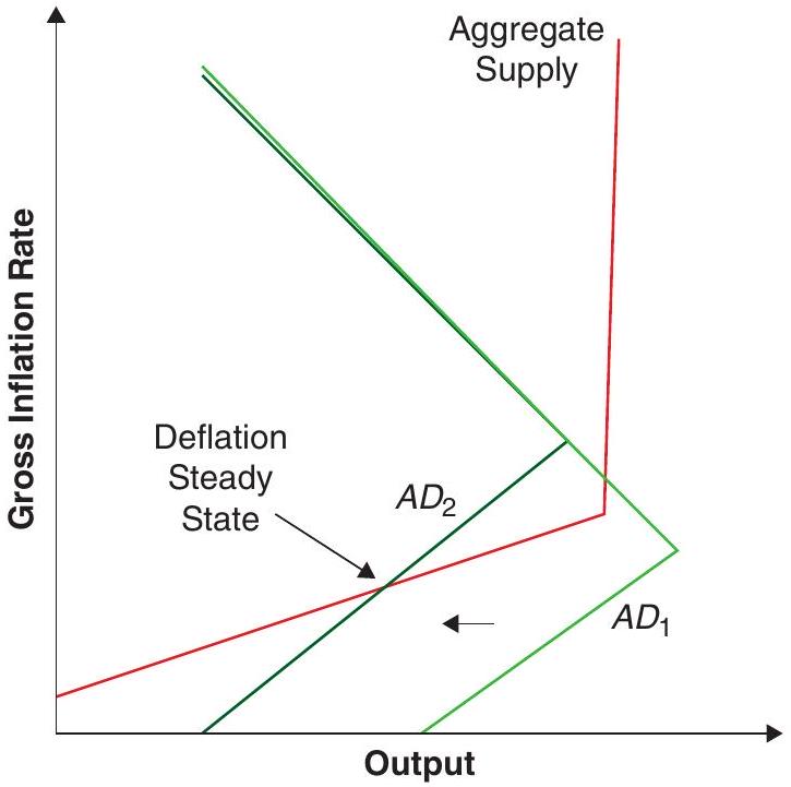
where \(Y^{f}\) represents full employment output. Notice that this operates as a Phillips curve, higher inflation is associated with higher output. The intuition is straightforward, as inflation increases the real wages falls and firms hire more labour. Given the rigidities of the model, this is a steady state relationship. If inflation is sufficiently high, the nominal wage rigidity does not bind and the aggregate supply becomes vertical, as drawn in Figure 22.1.
Aggregate demand follows directly from (22.7) combined with the Fisher relation (22.8) and a Taylor rule such as
\[ (1+i)=\left(1+i^{*}\right)\left(\frac{\Pi_{t}}{\Pi^{*}}\right)^{\phi_{\Pi}} . \tag{22.13}\]
Substituting both we obtain:
\[ Y=D+(2+\rho)(1+n) D \frac{\Pi^{*^{\phi_{\Pi}}}}{\left(1+i^{*}\right)} \frac{1}{\Pi^{\phi_{\Pi}-1}} . \tag{22.14}\]
The upper portion of the AD curve in Figure (22.1), when inflation is high and the interest rate is unconstrained, depicts this relationship. As inflation increases, the central bank raises the nominal interest rate by more than one for one (since \(\phi_{\Pi}>1\) ), which, in turn, increases the real interest rate and reduces demand.
Now, in low inflation states where the interest rate hits its zero lower bound \(i=0\), this curve simplifies to
\[ Y=D+(2+\rho)(1+n) D \Pi . \tag{22.15}\]
The key point of this equation is that it is upward sloping in \(\Pi\). The reason is straightforward, as inflation decreases, the lower bound implies that the real rate increases because the interest rate cannot compensate. Therefore, in this range, a lower inflation means a higher real rate. For reasonable parameter values the AD curve is steeper than the AS curve as in Figure 22.1
With this framework, imagine a decrease in \(D\). In (22.15) is is easy to see that this moves the aggregate demand to the left as shown in the graph. This pushes inflation and output downwards. The link between the financial crisis and a protracted stagnation process has been established.
22.2 The fiscal theory of the price level
Let’s imagine now a situation where people transact without money (in the current world of Venmo, electronic wallets, etc, this is not such a far-fetched assumption, and will become less and less farfetched as time goes by). What pins down the price level?2
The fiscal theory of the price level, as its name suggests, focuses on the role of fiscal policy in determining the price level. For sure, it is the government that prints money and issues debt. It then mops up money through taxes. To build intuition, let’s imagine the government issues debt that needs to be paid at the end of the period. Taxes will be used to that end and the fiscal result will be \(s_{t}\). Fiscal theory postulates that
\[ \frac{B_{t-1}}{P_{t}}=s_{t} . \tag{22.16}\]
The price level adjusts to equate the real value of debt to the expected surplus. Why is this the case? Imagine the price level is lower than the one that makes the real value of debt equal to the expected surplus. This means that at the end of the day the mopping up of money will be less than the value of debt. This implies that agents have an excess demand of resources to spend, which they use to push the price level up. If the price level makes the value of debt smaller than what will be mopped up, this implies that people are poorer and reduce spending. The price level comes down. In short, there is equilibrium when the real value of debt equals the expected surplus. Equation (22.16) is not the budget constraint of the government. The budget constraint is
\[ B_{t-1}=s_{t} P_{t}+M_{t} . \tag{22.17}\]
The point is that there is no demand for \(M_{t}\). This is what makes (22.16) an equilibrium condition. In the reasoning above we take \(s_{t}\) as exogenous, but we can also consider the case in which fiscal policy is endogenous in the sense that it adjusts in order to attain a particular \(P_{t}\). When so we will say we have a passive fiscal police. We will come back to this shortly.
Of course this intuition can be extended to multiple periods. In an intertemporal setting the budget constraint becomes
\[ M_{t-1}+B_{t-1}=P_{t} s_{t}+M_{t}+B_{t} E_{t}\left[\frac{1}{\left(1+i_{t}\right)}\right], \tag{22.18}\]
but because people do not hold money in equilibrium, and using the fact that \((1+i)=(1+\rho) \frac{P_{t+1}}{P_{t}}\) we can write this as
\[ B_{t-1}=P_{t} s_{t}+B_{t} E_{t}\left[\frac{1}{\left(1+i_{t}\right)}\right]=P_{t} s_{t}+B_{t} E_{t}\left[\frac{1}{(1+\rho)}\left(\frac{P_{t}}{P_{t+1}}\right)\right] . \tag{22.19}\]
It is easy to solve this equation by iterating forward (and assuming a transversality condition) to obtain
\[ \frac{B_{t-1}}{P_{t}}=E_{t} \sum_{j=0}^{\infty} \frac{s_{t+j}}{(1+\rho)^{j}} . \tag{22.20}\]
This equation pins down the price level as the interplay of the real value of debt and the present discounted value of expected fiscal surpluses. Again, the right-hand side is the amount of dollars to be mopped up. The left-hand side is the real value of the assets in the private sector’s hands. If the former is bigger than the future surpluses, there will be an aggregate demand effect that will push prices upward.
Imagine that the government issues debt but promises to increase the surpluses required to finance it. According to this view, this will have no effect on aggregate demand, or the price level. In fact, this explains why large fiscal deficits have had no effect on the price level. According to this view, to bring inflation up you need to issue debt and commit not to collect taxes! In short, you need to promise irresponsible behaviour. In Chris Sims’ (2016) words,
’Fiscal expansion can replace ineffective monetary policy at the zero lower bound, but fiscal expansion is not the same thing as deficit finance. It requires deficits aimed at, and conditioned on, generating inflation. The deficits must be seen as financed by future inflation, not future taxes or spending cuts.’
Notice that, under this light, a large increase in assets in the balance sheet of the central bank, (such as the quantitative easing exercises of last chapter), does not affect the price level. The government (the Fed) issues debt in exchange of commercial assets. If both assets and liabilities pay similar rates this does not affect future surpluses, it just adds assets and liabilities for the same amount. This result is not dissimilar to what happens when a Central Bank accumulates (foreign currency) reserves in fixed exchange rate regimes. An increase in money liabilities accompanied by an increase in backing is understood not to be inflationary. In summary in this framework the large expansions that have come with quantitative easing do not necessarily generate inflation pressures.
Finally, the FTPL shows the interplay between fiscal and monetary policy. Imagine a central bank that increases the interest rate. If the fiscal surplus does not change this would decrease the surpluses and generate inflation. The reason why typically it is not assumed that an increase rate in the interest increases inflation is due to the fact that it is assumed that an increase in the interest rate will lead automatically to an increase in the fiscal surplus in order to pay the higher interest cost. But, according to this view, this response is not necessary. It is an assumption that we make.
22.2.1 Interest rate policy in the FTPL
What does the FTPL have to say about the stability of interest rate policies? Let’s analyse this within the context of the New Keynesian model we discussed in Chapter 15. As always, the behavioural equations include the New Keynesian IS curve (NKIS):
\[ \log \left(Y_{t}\right)=E_{t}\left[\log \left(Y_{t+1}\right)\right]-\sigma\left(i_{t}-E_{t} \pi_{t+1}\right), \tag{22.21}\]
and the New Keynesian Phillips Curve (NKPC):
\[ \pi_{t}=\kappa y_{t}+\beta E_{t}\left[\pi_{t+1}\right] . \tag{22.22}\]
And an exogenous interest rule
\[ i_{t}=\bar{i} . \tag{22.23}\]
Notice that we use the exogenous interest rate rule that delivered instability in the traditional NK framework. The key innovation now is an equation for the evolution of the debt to GDP level in the model. The dynamics of the log of the debt to GDP can be approximated by
\[ d_{t+1}+s_{t+1}=d_{t}+\left(i_{t+1}-\pi_{t+1}\right)-g_{t+1} . \tag{22.24}\]
The debt to GDP ratio grows from its previous value with the primary deficit plus the real interest rate minus the growth rate.
The difference with the traditional NK model is that the NK model assumes that \(s_{t}\) adjusts to balance the budget to make debt sustainable, responding in a passive way, for example, to a change in the interest rate. This is the assumption that we lift here. Substituting the interest rate in the other equations we have a system of future variables on current variables with a coefficient matrix
\[ \Omega=\left[\begin{array}{lll} \frac{1}{\beta} & -\frac{\kappa}{\beta} & 0 \\ -\frac{\sigma}{\beta} & 1+\frac{\kappa \sigma}{\beta} & 0 \\ -\frac{1}{\beta} & \frac{\kappa}{\beta} & 1 \end{array}\right] . \tag{22.25}\]
The last column suggests that one of the eigenvalues is equal to one.3 Of the other two, one can be shown to be smaller than one, and the other larger than one. Because the system has two jumpy variables (output and inflation) and one state variable (debt), the system is stable.
The above may have sounded like a bit of mathematical jargon. But here we are interested in the economics of the model. First of all, what does the above mean? And then, why does the model uniquely pin down the equilibrium here?
Remember that in the standard NK model we needed the Taylor principle, an interest rule that reacted with strength to deviations in inflation to pin down the equilibrium. The above suggests the the Taylor principle is not necessary in this context. Here the equilibrium is stable even with relatively stable interest rates. But why is this the case? The key difference here is that the interest rate change does not lead to any reaction in fiscal policy. Typically we ignore the implications of monetary policy on the government’s budget constraint, but in doing so we are assuming (perhaps inadvertently) that fiscal policy responds automatically to monetary policy to keep the debt stable or sustainable. This may very well be the case, particularly in stable economies where fiscal stability is not at stake or questioned, but, at any rate, it is an assumption that we make.
What happens if we explicitly assume that there is no response of fiscal policy? Well, in that case the jump in the interest rate in an economy with sticky prices increases the real interest rate, but now there is only one path of inflation and output dynamics that insures the stability of the debt dynamics. The need to generate stability in the debt dynamics is what pins down the equilibria!
The increase in the real interest rate, though transitory, reduces the present value of surpluses (alternatively you can think of it as increasing the interest cost) leading to a higher level of inflation in equilibrium! The fact that higher interest rates imply a higher rate of inflation, is not necessarily contradictory with our previous findings, it just makes evident that in the previous case we were assuming that fiscal policy responded passively to insure debt stability.
The exercise helps emphasise that it is key to understand that relationship between fiscal and monetary policy. This relationship may become critical in the aftermath of the debt buildup as the result of Covid. If, imagine, interest rates increase at some point, what will be the response of fiscal policy? It is obvious that that channel cannot be ignored.
22.3 Rational asset bubbles
Our final topic is the role of bubbles in asset prices and their implications for the economy, both in terms of efficiency and stability.
Perhaps the right place to start is a standard asset-pricing arbitrage equation:
\[ r=\frac{\dot{q}_{t}}{q_{t}}+\frac{c}{q_{t}}, \tag{22.26}\]
where \(r\) is the real interest rate,4\(c\) the (constant) coupon payment, and \(q_{t}\) the price of the asset5. The equation states, as we have encountered multiple times, that the dividend yield plus the capital gain have to equal the opportunity cost of holding the asset.
That relationship can also be written as the differential equation
\[ \dot{q}_{t}=r q_{t}-c . \tag{22.27}\]
You may want to review in the mathematical appendix to check out that the solution of this differential equation has the form
\[ q_{t}=\int_{0}^{\infty} c e^{-r t} d t+B e^{r t}=\frac{c}{r}+B e^{r t}, \tag{22.28}\]
with \(B\) an arbitrary number (the fact that we use the letter \(B\) is not a coincidence). The solution has two terms. We call \(\frac{c}{r}\) the fundamental value of the asset (naturally, the present discounted value of the coupon stream). The term \(B e^{r t}\) is the bubble term, which has no intrinsic value. We sometimes refer to this term as a “rational bubble”.
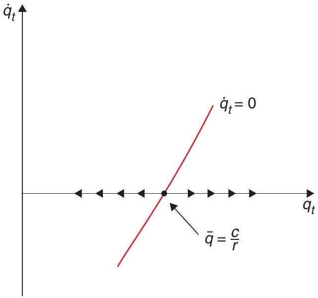
Unless we arbitrarily impose a terminal condition (like requiring that \(q\) does not exceed some boundary after some given time period), then every value of \(q\) that satisfies the differential equation above is a candidate solution. The set of possible solutions is shown in Figure 22.2, which graphs the dynamics of the differential equation.
If \(q\) starts to the right of \(\bar{q}\), it will go to infinity; if it starts to the left of \(\bar{q}\), it will go to zero. All these paths satisfy the relevant arbitrage condition and the corresponding differential equation.
Before moving on, one important point to note is that the bubble term has a very tight structure: it grows at \(r\). This is intuitive: the asset can price above its fundamental value only if agents expect this extra cost will also deliver the required rate of return … forever. Thus, transitory increases in asset prices cannot be associated with bubbles.6
Can we rule out these bubbly paths? If \(r>g\) - that is, the interest rate is larger than the growth rate - then the bubble eventually becomes so big that it is impossible for it to continue growing at the required rate (think of it becoming larger than the economy!). But if it cannot grow it cannot exist, and if it does not exist at a given moment in time by backward induction it cannot exist at anytime before. In dynamically efficient economies bubbles cannot exist.
That is the unsustainable element in bubbles; but there is also the de-stabilising element. Most borrowing contracts require collateral. Families use their homes as collateral; financial intermediaries use stocks and bonds as collateral. When the prices of these assets become inflated, so does people’s ability to borrow. So debt and leverage go up, which in turn may further stimulate the economy and causes asset prices to rise even more. The problem, of course, is that if and when asset prices come back to earth, it will find firms and businesses highly indebted, thus triggering a painful process of de-leveraging, recession, and bankruptcies.
So are bubbles all bad, then? Not necessarily. Imagine an overlapping generations ice cream economy in which people live for two days only. At any given time there are only two people alive: a 1-dayold person and a 2-day-old person. Each 1-day-old person gets an ice-cream cone in the evening. In this strange world, 1-day-olds do not like ice-cream, but 2-day-olds do. The problem is, anyone trying to store an ice cream cone overnight will only have a melted mess in her hands the next morning.
The 1-day-old person could kindly offer her cone to the 2 -day-old person, but the 2-day-old cannot offer anything in return, because they will be dead by morning. In this economy, therefore, one possible equilibrium is that all ice-cream melts and no one gets to eat any.
Unless, that is, one enterprising 2-day-old comes up with a new idea: give the 1-day-old a piece of paper (you can call it a dollar, or a bond if you prefer) in exchange for her cone, arguing that 24 hours later the then 2-day-old will be able to give that same piece of paper to a 1-day-old in exchange for a nice, fresh and un-melted ice cream cone! If today the 1-day-old agrees to the deal, and so do all successive 1-day-olds until kingdom come, then the problem will have been solved: all ice cream cones will be consumed by 2-day-olds who really appreciate their flavour, no ice cream will melt and welfare has improved.
But notice, the piece of paper that begins to change hands is like a bubble: it has no intrinsic value, and it is held only because of the expectation that others will be also willing to hold it in the future. In the simple story we have told the value of the bubble is constant: one piece of paper is worth one ice cream cone forever.7 But in slightly more complicated settings (with population growth, for instance, or with changing productivity in the ice cream business), the value of the piece of paper could be rising over time, or it could even be falling! People might willingly exchange one cone today for 0.9 cones tomorrow simply because the alternative is so bad: eating no ice cream at all!
You may have found a resemblance between this ice-cream story and our discussion of dynamic efficiency when analysing the overlapping generations models in Chapter 8. When the return on capital is low (in this case it is -100% because if everyone saves the ice-cream cone overnight, then there is no ice-cream to consume tomorrow), finding a way to transfer income from the young to old is welfare enhancing.
In Samuelson’s (1958) contribution that introduced the overlapping generations (OLG) model Samuelson already pointed out that bubble-like schemes (he called them “the social contrivance of money”) could get economies out of that dynamic inefficiency and raise welfare8.
But again, here is the rub: those schemes are inherently fragile. Each 1-day-old accepts the piece of paper if and only if they expect all successive 1-day-olds will do the same. If not, they have no incentive to do so. The conclusion is that, in a bubbly environment, even slight shifts in expectations can trigger big changes in behaviour and asset prices, what, in modern parlance, we call financial crises.
In another very celebrated paper, Samuelson’s fellow Nobelist Jean Tirole (1985) took a version of the OLG model and analysed what kinds of bubbles could arise and under what conditions. The main conclusion is what we mentioned above: rational asset bubbles only occur in low interest rate OLG economies where the rate of interest is below the rate of growth of the economy. This is how Weil (2008) explains the intuition:
’This result should not be a surprise: I am willing to pay for an asset more than its fundamental value (the present discounted value of future dividends) only if I can sell it later to others. A rational asset bubble, like Samuelsonian money, is a hot potato that I only hold for a while-until I find someone to catch it.’
Tirole’s paper gave rise to a veritable flood of work on bubbles, rational and otherwise. Recent surveys covering this new and fast-growing literature are Miao (2014) and Martin and Ventura (2018). One result from that literature is that there is nothing special in the 2 -generation Samuelson model that generates bubbles. Overlapping generations help, but other kinds of restrictions on trade (which is, essentially, what the OLG structure involves) can deliver very similar results.
In what follows we develop a simple example of rational bubbles using the Blanchard-Yaari perpetual youth OLG model that we studied in Chapter 8. In building this model we draw on recent work by Caballero et al. (2008), Farhi and Tirole (2012) and Galí (2020).
22.3.1 The basic model
Consider an economy made up of overlapping generations of the Blanchard type with ageindependent probability of death \(p\) (which by the law of large numbers is also the death rate in the population) and birth rate \(n>p\). Together they mean population grows at the rate \(n-p\). As in Blanchard (1985), assume there exist insurance companies that allow agents to insure against the risk of death (and, therefore, of leaving behind unwanted bequests)9.
Let \(r_{t}\) be the interest rate and \(\rho\) the subjective rate of time discounting. Starting on the day of their birth, agents receive an endowment that cannot be capitalised and that declines at the rate \(\gamma>\rho\). It is this assumption that income goes down as agents get older that will create a demand for a savings vehicle in order to move purchasing power from earlier to later stages of life.
The per capita (or, if you prefer, average) endowment received by agents who are alive at time \(t\) is (see Appendix 1 for details) a constant \(y\).
Next let \(h_{t}\) stand for per capita (or average) household wealth. Appendix 2 shows that \(h_{t}\) evolves according to
\[ \dot{h}_{t}=\left(r_{t}+p+\gamma\right) h_{t}-y . \tag{22.29}\]
To develop some intuition for this last equation, it helps to think of \(h_{t}\) as the present per capita value of the income flow \(y\) the household receives. What is the relevant rate at which the household should discount those future flows? The total discount rate is \(\left(r_{t}+p+\gamma\right)\). In addition to the standard rate of interest \(r_{t}\), the household must also discount the future by \(p\), the instantaneous probability of death, and by \(\gamma\), which is the rate at which an individual’s income falls over time.
The only way to save is to hold a bubble, whose per capita value is \(b_{t}\). Arbitrage requires that per capita gains on the value of the bubble equal the interest rate:
\[ \frac{\dot{b}_{t}}{b_{t}}=r_{t}-(n-p) . \tag{22.30}\]
Recall that \(b_{t}\) is the per capita stock of the bubble, and \((n-p)\) is the rate of population growth. So this equation says that, by arbitrage, the percentage rate of growth of the (per capita) bubble must be equal to the (per capita) return on financial assets, which equals the interest rate net of population growth.
Finally, if utility is logarithmic, then (see Appendix 3) the per capita consumption function is
\[ c_{t}=(p+\rho)\left(b_{t}+h_{t}\right), \tag{22.31}\]
so that consumption is a fixed portion of household wealth and financial wealth (the bubble). This condition mimics those we found for all Ramsey problems with log utility as we know from earlier chapters of this book. Because the economy is closed, all output must be consumed. Market-clearing requires
\[ c_{t}=y=(p+\rho)\left(b_{t}+h_{t}\right) . \tag{22.32}\]
Therefore, differentiating with respect to time we have
\[ \dot{b}_{t}+\dot{h}_{t}=0 . \tag{22.33}\]
Replacing (22.29) and (22.30) in (22.33) yields
\[ \left(r_{t}+p+\gamma\right) h_{t}+\left(r_{t}+p-n\right) b_{t}=y . \tag{22.34}\]
Combining this equation with the market-clearing condition (22.32) we get after some simplifications
\[ r_{t}+\gamma-\rho=\frac{(p+\rho)(n+\gamma) b_{t}}{y}, \tag{22.35}\]
so that \(r_{t}\) is increasing in \(b_{t}\) : a larger bubble calls for a higher interest rate. Next we can use this equation to eliminate \(r_{t}-n\) from the arbitrage equation (22.30) that governs the bubble:
\[ \dot{b}_{t}=\frac{(p+\rho)(n+\gamma) b_{t}^{2}}{y}-(n-p+\gamma-\rho) b_{t} . \tag{22.36}\]
It follows that \(\dot{b}_{t}=0\) implies
\[ [(p+\rho)(n+\gamma) b-(n-p+\gamma-\rho) y] b=0 . \tag{22.37}\]
This equation has solutions \(b=0\) and
\[ b=\frac{(n-p+\gamma-\rho) y}{(p+\rho)(n+\gamma)}>0 . \tag{22.38}\]
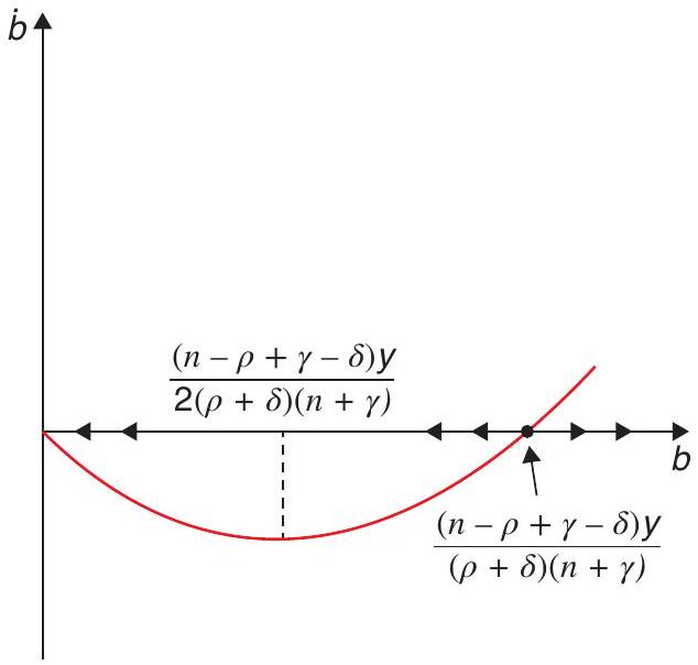
Figure 22.3 describes the dynamic behaviour of the bubble. There are two steady states. The one with \(b=0\) is stable, while the one with with \(b>0\) is unstable. So bubbles can exist, but they are very fragile. Starting from the bubbly steady state, a minuscule shift in expectations is enough to cause the value of the bubble to start declining until it reaches zero.
Because this is a closed economy, per capita consumption must be equal to per capita income. But the same is not true of the consumption profiles of individual cohorts. It is easy to check that, in the bubbly steady state individual cohort consumption grows over time, while in the non-bubbly steady state, individual cohort consumption is flat. The bubble amounts to a savings vehicle that allows individuals to push consumption to later stages of life.
Put differently, in the steady state with no bubble, the interest rate is negative (you can see that the interest rate is \(\rho-\gamma<0\) by just assuming \(b=0\) in (22.35)). This is, trivially, smaller than the rate of population growth \((n-p)>0\). So in that steady state the economy is dynamically inefficient. The existence of a bubble allows the economy to escape that inefficiency and settle on a golden rule steady state in which the interest rate is equal to the rate of population growth (to check this replace the level of \(b\) from (22.38) in (22.35) to find that \(r=n-p\) ). But that equilibrium is fragile, as we have seen.
22.3.2 Government debt as a bubble
Now define \(d_{t}\) as per capita public debt. The government budget constraint is
\[ \dot{d}_{t}=\left(r_{t}-n+p\right) d_{t}+s, \tag{22.39}\]
where \(s\) is constant net spending per capita - the equivalent of the per capita primary deficit. Assume that all government spending is transfers to households (as opposed to government consumption), so the law of motion of household wealth must be modified to read
\[ \dot{h}_{\mathrm{t}}=\left(r_{t}+p+\gamma\right) h_{t}-y-s . \tag{22.40}\]
The consumption function is still (22.32), and \(c_{t}=y\) which again implies that \(\dot{h}_{t}+\dot{d}_{t}=0\). We can then repeat the steps in the previous subsection replacing \(b_{t}\) by \(d_{t}\) to get an expression for the interest rate as a function of \(d_{t}\) :
\[ \left(r_{t}+\gamma-\rho\right) y=(n+\gamma)(p+\rho) d_{t}, \tag{22.41}\]
which is virtually identical to (22.35). As before \(r_{t}\) is increasing in \(d_{t}\) : a larger stock of government debt requires a higher interest rate. Using this last expression in the government budget (22.39) constraint to eliminate \(r_{t}-n\) we have
\[ \dot{d}_{t}=\left(r_{t}-n+p\right) d_{t}+s=y^{-1}(n+\gamma)(p+\rho) d_{t}^{2}-(n-p+\gamma-\rho) d_{t}+s . \tag{22.42}\]
Notice \(\dot{d}_{t}=0\) implies
\[ (n+\gamma)(p+\rho) d^{2}-(n-p+\gamma-\rho) y d+s y=0 . \tag{22.43}\]
This equation has two solutions, given by
\[ \frac{d}{y}=\frac{(n-p+\gamma-\rho) \pm \sqrt{(n-p+\gamma-\rho)^{2}-4(n+\gamma)(p+\rho) \frac{s}{y}}}{2(n+\gamma)(p+\gamma)} . \tag{22.44}\]
Solutions exist as long as spending does not exceed a maximum allowable limit, given by
\[ s=\frac{(n-p+\gamma-\rho)^{2} y}{4(n+\gamma)(p+\rho)} . \tag{22.45}\]
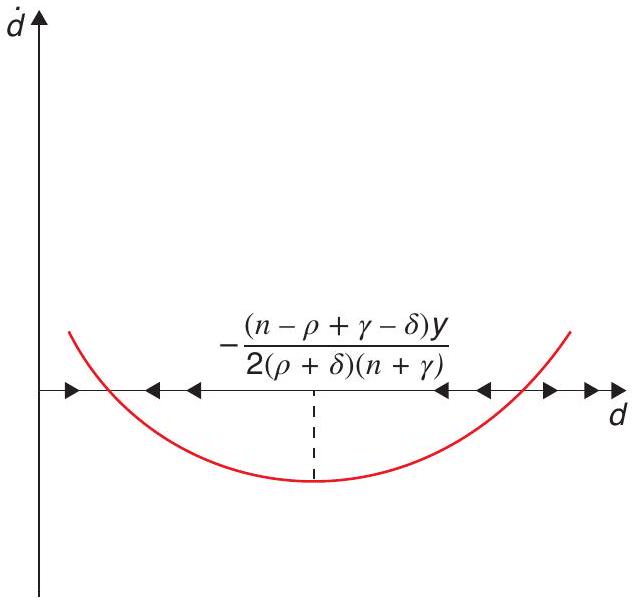
If \(s\) is below this maximum, we have two equilibria, both with positive levels of debt. Figure (22.4) confirms that in this case the bubble is fragile: the steady state with the larger stock of debt is unstable. A slight shift in expectations will cause the value of the bubble to start declining.
It is straightforward to show that there are also two solutions for the real interest rate, given by
\[ r=\frac{(n-p)-(\gamma-\rho) \pm \sqrt{((n-p)+(\gamma-\rho))^{2}-4(n+\gamma)(p+\rho) \frac{s}{y}}}{2} . \tag{22.46}\]
If \(s=0\), then
\[ r=\frac{(n-p)-(\gamma-\rho) \pm((n-p)+(\gamma-\rho))}{2}, \tag{22.47}\]
so \(r=n-p\) or \(r=-(\gamma-\rho)\), just as in the case of a pure bubble.
If \(s>0\), then in both equilibria \(r<n-p\), so government debt turns out to be a bubble. In either steady state, the government budget constraint is
\[ (n-p-r) d=s . \tag{22.48}\]
When the steady state interest rate is higher, so is the steady state value of the debt for a given primary deficit. One steady state is bubblier, with a larger valuation for public debt and a higher interest rate. But that steady state, as we saw graphically in the phase diagram above, is fragile. It only takes a shift in expectations to drive the economy out of that resting place and toward the alternative steady state with a lower valuation for public debt.
22.3.3 Implications for fiscal, financial and monetary policy
As the discussion in the previous section should make clear, bubbles have huge implications for fiscal policy. We saw that in an economy with strong demand for liquidity, private sector agents may be willing to hold government debt even if that debt pays an interest rate that is lower than the rate of population growth, which is also the rate of growth of the economy.
This is good news for treasury officials and fiscal policymakers: the model suggests, they can run a primary deficit forever without ever having to raise taxes to retire the resulting debt. This is not just a theoretical curiosum. Today in most advanced economies, the real rate of interest is below the rate of economic growth (however paltry that rate of growth may be). This fact is motivating a deep rethinking about the limits of fiscal policy and the scope for a robust fiscal response not only to the Covid-19 pandemic, but also to the green infrastructure buildup that global warming would seem to require. Olivier Blanchard devoted his Presidential Lecture to the American Economic Association (2019) to argue that a situation in which \(r<g\) for a prolonged period of time opens vast new possibilities for the conduct of fiscal policy10.
But, at the same time, a bubbly world also bears bad news for those in charge of fiscal policy because, as we have seen above, bubbly equilibria are inherently fragile. Could it be that an advanced country issues a great deal of debt at very low interest rates and one day investors decide to dump it simply because of a self-fulfilling change in expectations? Hard to say, but it is not a possibility that can be entirely ignored. In fact, Blanchard (2019) acknowledges that arguments based on the possibility of multiple equilibria are “the most difficult to counter” when making the case for the increased fiscal space that low interest rates bring.
Bubbles also have vast implications for financial markets and financial regulation. The obvious concern, mentioned at the outset, is that asset bubbles typically end in tears, with overvaluation abruptly reversing itself and wrecking balance sheets. But here, also, the news is not all bad. Financial markets typically involve inefficient borrowing constraints that keep a subset of agents (especially small and medium enterprises) from undertaking positive net-present-value projects. Therefore, as Martin
and Ventura (2018) emphasise, to the extent that bubbles pump up the value of collateral and relax borrowing constraints, they can promote efficiency and raise welfare as long as those bubbles do not burst11.
Last but certainly not least, bubbles present difficult dilemmas for central banks and for monetary policy more generally. In the presence of sticky prices, if bubbles affect aggregate demand they also affect output and inflation, giving rise to bubble-driven business cycles. The implication is that standard monetary and interest rate rules need to be modified to take into account this new source of fluctuations. In some cases those modifications are relatively minor, but that is not always the case. Galí (2020) discusses the issues involved in greater detail than we can here.
22.4 Appendix 1
Let \(N_{t, \tau}\) be the size at time \(t\) of the cohort born at \(\tau\). The initial size of the cohort born at \(\tau\) is \(n N_{\tau}\). In addition, the probability that someone born at \(\tau\) is still alive at \(t \geq \tau\) is \(e^{-p(t-\tau)}\). It follows that
\[ N_{t, \tau}=n N_{\tau} e^{-p(t-\tau)} . \tag{22.49}\]
Now, \(N_{t}=N_{\tau} e^{(n-p)(t-\tau)}\), so
\[ \frac{N_{t, \tau}}{N_{t}}=n e^{-p(t-\tau)} e^{-(n-p)(t-\tau)}=n e^{-n(t-\tau)} . \tag{22.50}\]
We conclude the relative size at time \(t\) of the cohort born at \(\tau\) is \(n e^{-n(t-\tau)}\) For any variable \(x_{t, \tau}\) define the per capita (or average) \(x_{t}\) as
\[ x_{t}=\int_{-\infty}^{t} x_{t, \tau}\left(\frac{N_{t, \tau}}{N_{t}}\right) d \tau, \tag{22.51}\]
\[ x_{t}=\int_{-\infty}^{t} x_{t, \tau} n e^{-n(t-\tau)} d \tau . \tag{22.52}\]
For a person belonging to the cohort born on date \(\tau\), endowment income at time \(t\) is
\[ y_{t, \tau}=\left(\frac{n+\gamma}{n}\right) y e^{-\gamma(t-\tau)}, \tag{22.53}\]
where \(y\) is a constant. Next define per capita (or average) endowment at time \(t\) as
\[ y_{t}=\int_{-\infty}^{t} y_{t, \tau} n e^{-n(t-\tau)} d \tau \tag{22.54}\]
\[ y_{t}=y\left(\frac{n+\gamma}{n}\right) \int_{-\infty}^{t} e^{-\gamma(t-\tau)} n e^{-n(t-\tau)} d \tau, \tag{22.55}\]
\[ y_{t}=y(n+\gamma) \int_{-\infty}^{t} e^{(n+\gamma)(t-t)} d \tau, \tag{22.56}\]
\[ y_{t}=y . \tag{22.57}\]
22.5 Appendix 2
The following derivation follows Blanchard (1985). Let the human wealth at time \(t\) of someone born on date \(\tau\) be
\[ h_{t, \tau}=\int_{t}^{\infty} y_{s, \tau} e^{-\int_{t}^{s}\left(r_{v}+p\right) d v} d s \tag{22.58}\]
The income at time \(s\) of an individual is born on date \(\tau\) is (this is the key declining income path assumption)
\[ y_{s, \tau}=\left(\frac{n+\gamma}{n}\right) y e^{-\gamma(s-\tau)}=\left(\frac{n+\gamma}{n}\right) y e^{-\gamma(s-t)} e^{\gamma(t-t)} . \tag{22.59}\]
Therefore, the expression for \(h_{t, \tau}\) can be written
\[ h_{t, \tau}=e^{\gamma(\tau-t)} \int_{t}^{\infty}\left(\frac{n+\gamma}{n}\right) y e^{-\int_{t}^{s}\left(r_{v}+p+\gamma\right) d v} d s . \tag{22.60}\]
Next define per capita (or average) human wealth held by those still alive at \(t\), given by
\[ h_{t}=\int_{-\infty}^{t} h_{t, \tau} n e^{n(\tau-t)} d \tau . \tag{22.61}\]
Using the expression for \(h_{t, \tau}\) the last equation can be written as
\[ h_{t}=\int_{-\infty}^{t} e^{\gamma(\tau-t)}\left\{\int_{t}^{\infty}\left(\frac{n+\gamma}{n}\right) y e^{-\int_{t}^{s}\left(r_{v}+p+y\right) d v} d s\right\} n e^{n(\tau-t)} d \tau, \tag{22.62}\]
where the expression in curly brackets is the same for all agents. It follows that
\[ h_{t}=\left\{\int_{t}^{\infty} y e^{-\int_{t}^{s}\left(r_{v}+p+\gamma\right) d v} d s\right\}(n+\gamma) \int_{-\infty}^{t} e^{(n+\gamma)(\tau-t)} d \tau, \tag{22.63}\]
\[ h_{t}=\int_{t}^{\infty} y e^{-\int_{t}^{s}\left(r_{v}+p+\gamma\right) d v} d s \tag{22.64}\]
Finally, differentiating with respect to time \(t\) we arrive at
\[ \dot{h}_{t}=\left(r_{t}+p+\gamma\right) h_{t}-y, \tag{22.65}\]
which is the equation of motion for human capital in the text.
22.6 Appendix 3
One can show the individual Euler equation at time \(t\) for an agent born at date \(s\) is
\[ \dot{c}_{t, \tau}=c_{t_{t} \tau}\left(r_{t}-\rho\right) . \tag{22.66}\]
The present-value budget constraint of this agent is
\[ \int_{t}^{\infty} c_{s, \tau} e^{-\int_{t}^{s}\left(r_{v}+p\right) d v} d s=b_{t, \tau}+h_{t, \tau} . \tag{22.67}\]
Using the Euler equation here, we have
\[ c_{t, \tau} \int_{t}^{\infty} e^{\int_{t}^{s}\left(r_{v}-\rho\right) d v} e^{-\int_{t}^{s}\left(r_{v}+\rho\right) d v} d s=b_{t, \tau}+h_{t, \tau} \tag{22.68}\]
\[ c_{t, \tau} \int_{t}^{\infty} e^{-(p+\rho)(s-t)} d s=b_{t, \tau}+h_{t, \tau} \tag{22.69}\]
\[ c_{t, \tau}=(p+\rho)\left(b_{t, \tau}+h_{t, \tau}\right) \tag{22.70}\]
Next derive the per capita consumption function, given by
\[ c_{t}=\int_{-\infty}^{t} c_{t, \tau} n e^{-n(t-\tau)} d \tau . \tag{22.71}\]
Using (22.70) this becomes
\[ c_{t}=(p+\rho) \int_{-\infty}^{t}\left(b_{t, \tau}+h_{t, \tau}\right) n e^{-n(t-\tau)} d \tau, \tag{22.72}\]
\[ c_{t}=(p+\rho) \int_{-\infty}^{t} b_{t, \tau} n e^{-n(t-\tau)} d \tau+(p+\rho) \int_{-\infty}^{t} h_{t, \tau} n e^{-n(t-\tau)} d \tau, \tag{22.73}\]
\[ c_{t}=(p+\rho)\left(b_{t}+h_{t}\right), \tag{22.74}\]
which is the per capita (or average) consumption function.
References
Acemoglu, D. (2009). Introduction to modern economic growth. Princeton University Press.
Blanchard, O. (2019). Public debt and low interest rates. American Economic Review, 109(4), 1197-1229.
Blanchard, O. J. (1985). Debt, deficits, and finite horizons. Journal of Political Economy, 93(2), 223-247.
Caballero, R. J., Farhi, E., & Gourinchas, P.-O. (2008). An equilibrium model of “global imbalances” and low interest rates. American Economic Review, 98(1), 358-93.
Caballero, R. J. & Krishnamurthy, A. (2006). Bubbles and capital flow volatility: Causes and risk management. Journal of Monetary Economics, 53(1), 35-53.
Chodorow-Reich, G., Gopinath, G., Mishra, P., & Narayanan, A. (2020). Cash and the economy: Evidence from India’s demonetization. The Quarterly Journal of Economics, 135(1), 57-103.
Cochrane, J. H. (2021). The fiscal theory of the price level. Manuscript. URL https://www.johnhcochrane.com/research-all/the-fiscal-theory-of-the-price-level-1.
Farhi, E. & Tirole, J. (2012). Bubbly liquidity. The Review of Economic Studies, 79(2), 678-706.
Galí, J. (2020). Monetary policy and bubbles in a New Keynesian model with overlapping generations. National Bureau of Economic Research.
Martin, A. & Ventura, J. (2018). The macroeconomics of rational bubbles: A user’s guide. Annual Review of Economics, 10, 505-539.
Miao, J. (2014). Introduction to economic theory of bubbles. Journal of Mathematical Economics, 53, 130-136.
Reis, R. (2020). The constraint on public debt when \(\mathrm{r}<\mathrm{g}\) but \(\mathrm{g}<\mathrm{m}\).
Rogoff, K. S. (2016). The curse of cash. Princeton University Press.
Samuelson, P. A. (1958). An exact consumption-loan model of interest with or without the social contrivance of money. Journal of Political Economy, 66(6), 467-482.
Sims, C. A. (2016). Fiscal policy, monetary policy and central bank independence. https://bit.ly/3BmMJYE.
Tirole, J. (1985). Asset bubbles and overlapping generations. Econometrica, 1499-1528.
Weil, P. (2008). Overlapping generations: The first jubilee. Journal of Economic Perspectives, 22(4), 115-34.
Economists such as Ken Rogoff have been advocating the phasing out of cash, see Rogoff (2016). Recently, India implemented a drastic reduction of cash availability, which is analysed in Chodorow-Reich et al. (2020).↩︎
This section follows mostly the work of John Cochrane as presented in his book Cochrane (2021), to which we refer for those interested in further exploration of this topic.↩︎
If you find this statement confusing, remember that to find the characteristic equation you need to find the determinant of this matrix. Expanding by the last column means that the equation is \(1-\lambda\) times the determinant of the upper left quadrant. This quickly indicates that 1 is one of the eigenvalues.↩︎
Actually, the opportunity cost of an asset with similar risk characteristics.↩︎
The assumption of a constant coupon is done for simplification but in no way necessary.↩︎
Another interesting point is that if the bubble bursts, its value goes to zero: there is no gradual undoing of a bubble. Thus, the pattern of the unwinding of an asset price will tell you a lot about whether the previous surge was or was not a bubble or just a change in the perception on fundamentals.↩︎
In the framework of (22.28) this would be a case in which the interest rate is zero.↩︎
For a crystal-clear explanation of this see Weil (2008), on which this introduction draws.↩︎
This is a slightly simplified version of the same model we presented in Chapter 8 and here follows Acemoglu (2009). Rather than having you go back to that model we have moved some computations to three appendices of this chapter for ease of reference.↩︎
On the same topic, see also Reis (2020).↩︎
Caballero and Krishnamurthy (2006) explore this tension in the context of bubbly capital flows to emerging markets.↩︎