21 Recent debates in monetary policy
In the last two chapters we presented the basic analytics of monetary policy in the long and in the short run. For the short run, we developed a simple New Keynesian model that can parsimoniously make sense of policy as it has been understood and practised over the last few decades.
Before the 2008 financial crisis, most advanced-country central banks, and quite a few emergingmarket central banks as well, carried out monetary policy by targeting a short-term interest rate. In turn, movements in this interest rate were typically guided by the desire to keep inflation close to a predefined target - this was the popular policy of inflation targeting. This consensus led to a dramatic decrease in inflation, to the point of near extinction in most economies, over the last two or three decades.
But this benign consensus was shaken by the Great Financial Crisis of 2008-2009. First, there was criticism that policy had failed to prevent (and perhaps contributed to unleashing) the crisis. Soon, all of the world’s major central banks were moving fast and courageously into uncharted terrain, cutting interest rates sharply and all the way to zero. A first and key issue, therefore, was whether the conventional tools of policy had been rendered ineffective by the zero lower bound.
In response to the crisis, and in a change that persists until today, central banks adopted all kinds of unconventional or unorthodox monetary policies. They have used central bank reserves to buy Treasury bonds and flood markets with liquidity, in a policy typically called quantitative easing. And they have also used their own reserves to buy private sector credit instruments (in effect lending directly to the private sector) in a policy often referred to as credit easing.
Interest rate policy has also become more complex. Central banks have gone beyond controlling the contemporary short rate, and to announcing the future path of short rates (for a period of time that could last months or years), in an attempt at influencing expectations a policy known as forward guidance. Last but not least, monetary authorities have also begun paying interest on their own reserves - which, to the extent that there is a gap between this rate and the short-term market rate of interest (say, on bonds), gives central bankers an additional policy tool.
These policies can be justified on several grounds. One is the traditional control of inflation - updated in recent years to include avoidance of deflation as well. Another is control of aggregate demand and output, especially when the zero lower bound on the nominal interest limits the effectiveness of traditional monetary policy. A third reason for unconventional policies is financial stability: if
spikes in spreads, for instance, threaten the health of banks and other financial intermediaries (this is exactly what happened in 2007-09), then monetary policy may need to act directly on those spreads to guarantee stability and avoid runs and the risk of bankruptcy.
Do these policies work, in the sense of attaining some or all of these objectives? How do they work? Why do they work? What does their effectiveness (or lack of effectiveness) hinge on?
A massive academic literature on these questions has emerged during the last decade. Approaches vary, but the most common line of attack has been to append a financial sector to the standard New Keynesian model (yes, hard to believe, but, until the crisis, finance was largely absent from most widely-used macro models), and then explore the implications.
This change brings at least two benefits. First, finance can itself be a source of disturbances, as it occurred in 2007-09 and had also occurred in many earlier financial crises in emerging markets. Second, the enlarged model can be used to study how monetary policy can respond to both financial and conventional disturbances, with the financial sector also playing the role of potential amplifier of those shocks.
Here we cannot summarise that literature in any detail (but do look at Eggertsson and Woodford (2003), Gertler and Karadi (2011), and the survey by Brunnermeier et al. (2013) for a taste). What we do is extend our standard NK model of earlier sections and chapters to include a role for liquidity and finance, and we use the resulting model to study a few (not all) varieties of unconventional monetary policy.
The issues surrounding conventional and unconventional monetary policies have taken on new urgency because of the Covid-19 crisis. In the course of 2020, central banks again resorted to interest, cutting it all the way to the zero lower bound, coupled with quantitative easing and credit easing policies that are even more massive than those used over a decade ago. And in contrast to the Great Financial Crisis, when only advanced-country central banks experimented with unconventional policies, this time around many emerging-economy central banks have dabbled as well. So understanding how those policies work has key and urgent policy relevance - and that is the purpose of this chapter.
21.1 The liquidity trap and the zero lower bound
John Hicks, in the famous paper where he introduced the IS-LM model (1937), showed how monetary policy on occasion might become ineffective. These “liquidity traps” as he called them, occurred when the interest rate fell to zero and could not be pushed further down. In this section we model this liquidity trap in our New Keynesian framework.
Until not too long ago, economists viewed the liquidity trap as the stuff of textbooks, not reality. But then in the 1990s Japan got stuck in a situation of very low or negative inflation and no growth. No matter what the Japanese authorities tried, nothing seemed to work. In 1998, Paul Krugman pointed out that “here we are with what surely looks a lot like a liquidity trap in the world’s second-largest economy”. And then he proceeded to show that such a trap could happen not just in the static IS-LM model, but in a more sophisticated, dynamic New Keynesian model.
Of course, the experience of Japan was not the only one in which a liquidity trap took center stage. During the world financial crisis of 2008-09, the world’s major central banks cut their interests to zero or thereabouts, and found that policy alone was not sufficient to contain the collapse of output. The same, perhaps with greater intensity and speed, has occurred during the Covid-19 crisis of 2020-21,
with monetary authorities cutting rates to zero and searching for other policy tools to contain the destruction of jobs and the drop in activity. So, the issues surrounding the zero lower bound and liquidity traps are a central concern of macroeconomists today1.
To study such traps formally, let us return to the two-equation canonical New Keynesian model of Chapter 15
\[ \dot{\pi}_{t}=\rho \pi_{\mathrm{t}}-\kappa x_{t}, \tag{21.1}\]
\[ \dot{x}_{\mathrm{t}}=\sigma\left(i_{t}-\pi_{\mathrm{f}}-r^{n}\right), \tag{21.2}\]
where, recall, \(\pi_{t}\) is inflation, \(x_{t}\) is the output gap, \(i_{t}\) is the policy-determined nominal interest rate, \(r^{n} \equiv \rho+\sigma^{-1} g\) is the natural or Wicksellian interest rate, which depends on both preferences (the discount rate \(\rho\) and the elasticity \(\sigma\) ) and trend productivity growth ( \(g\) ).
To close the model, instead of simply assuming a mechanic policy rule (of the Taylor type or some other type, as we did in Chapter 15), we consider alternative paths for the interest rate in response to an exogenous shock. Werning (2011), in an influential and elegant analysis of the liquidity trap, studies formal optimisation by the policymaker, both under rules and under discretion. Here we take a somewhat more informal approach, which draws from his analysis and delivers some of the same policy insights.2
Define a liquidity trap as a situation in which the zero lower bound is binding and monetary policy is powerless to stabilise inflation and output. To fix ideas, consider the following shock:
\[ r_{\mathrm{t}}^{n}=\left\{\begin{array}{l} \underline{r}^{n}<0 \text { for } 0 \leq t<T \\ r^{n}>0 \text { for } t \geq T . \end{array}\right. \tag{21.3}\]
Starting from \(r^{n}\), at time 0 the natural rate of interest unexpectedly goes down to \(\underline{r}^{n}\), and it remains there until time \(T\), when it returns to \(r^{n}\) and stays there forever. The key difference between this shock and that studied in Chapter 15 in the context of the same model, is that now the natural rate of interest is negative for an interval of time. Recall that this rate depends on preferences and on trend growth in the natural rate of output. So if this productivity growth becomes sufficiently negative, \(r_{t}^{n}\) could be negative as well.
Notice that the combination of flagging productivity and a negative natural rate of interest corresponds to what Summers (2018) has labelled secular stagnation. The point is important, because, if secular stagnation, defined by Summers precisely as a situation in which the natural rate of interest falls below zero for a very long time (secular comes from the Latin soeculum, meaning century), then economies will often find themselves in a liquidity trap.
The other novel component of the analysis here, compared to Chapter 15, is that now we explicitly impose the zero lower bound on the nominal interest rate, and require that \(i_{t} \geq 0 \forall t\).
If the central bank acts with discretion, choosing its preferred action at each instant, the zero lower bound will become binding as it responds to the shock. To see this, let us first ask what the central bank will optimally do once the shock is over at time \(T\). Recall the canonical New Keynesian model displays, what Blanchard and Galí (2007) called the divine coincidence: there is no conflict between keeping inflation low and stabilising output. If \(i=r^{n}\), then \(\pi_{t}=x_{t}=0\) is an equilibrium. So starting at time \(T\), any central bank that is happiest when both inflation and the output gap are at zero will engineer exactly that outcome, ensuring \(\pi_{t}=x_{t}=0 \quad \forall t \geq T\).
In terms of the phase diagram in Figure 21.1, we assume that initially (before the shock) \(i=r^{n}\), so that \(\pi_{t}=0 \forall t<0\). Therefore, the initial steady state was at point A, and to that point exactly the system must return at time \(T\). What happens between dates 0 and \(T\) ? Trying to prevent a recession and the corresponding deflation, the central bank will cut the nominal interest all the way to zero. That will mean that between dates 0 and \(T\), dynamics correspond to the system with steady state at point D, but because of the zero lower bound, policy cannot take the economy all the way back to the pre-shock situation and keep \(\pi_{t}=x_{t}=0\) always. So, on impact the system jumps to point B, and both inflation and the output gap remain negative (deflation and depression or at least recession take hold) in the aftermath of the shock and until date \(T\)3.
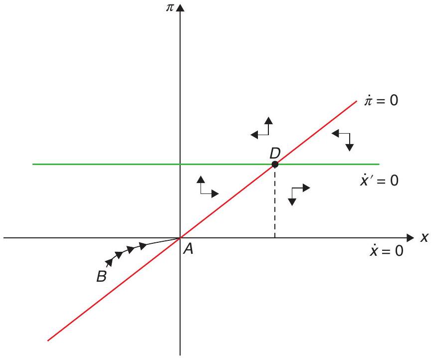
Both Krugman (1998) and Werning (2011) emphasise that the problem is the central bank’s lack of credibility: keeping the economy at \(\pi_{t}=x_{t}=0\) is optimal starting at time \(T\), and so people in this economy will pay no attention to announcements by the central bank that claim something else. In technical language, the monetary authority suffers from a time inconsistency problem of the kind identified by Kydland and Prescott (1977) and Calvo (1978) (see Chapter 20): from the point of view of any time before time \(T\), engineering some inflation after \(T\) looks optimal. But when time \(T\) arrives, zero inflation and a zero output gap become optimal.
What is to be done? This is Krugman’s (1998) answer: The way to make monetary policy effective, then, is for the Central Bank to credibly promise to be irresponsible - to make a persuasive case that it will permit inflation to occur, thereby producing the negative real interest rates the economy needs. In fact, there are simple paths for the nominal interest rate that, if the central bank could commit to them, would deliver a better result. Consider a plan, for instance, that keeps inflation and the output gap constant at
\[ \pi_{t}=-\underline{r}^{n}>0 \text { and } x_{t}=-\frac{\underline{r}^{n}}{\kappa}>0 \quad \forall t \geq 0 . \tag{21.4}\]
Since \(i_{t}=r_{t}^{n}+\pi_{t}\), it follows that \(i_{t}=0 \quad \forall t<T\), and \(i_{t}=r^{n}-\underline{r}^{n}>0 \quad \forall t \geq T\). Although this policy is not fully optimal, it may well (depending on the social welfare function and on parameter values) deliver higher welfare than the policy of \(i_{t}=0\) forever, which causes recession and deflation between
0 and \(T\). And note that as prices become less sticky (in the limit, as \(\kappa\) goes to infinity), the output gap goes to zero, so this policy ensures no recession (and no boom either)4.
Notice, strikingly, that this policy - just like the one described in the phase diagram above - also involves keeping the nominal interest stuck against the zero lower bound during the whole duration of the adverse shock, between times 0 and \(T\). So if the policy is the same over that time interval, why are results different? Why is there no recession as a result of the shock? Crucially, the difference arises because now people expect there will be inflation and a positive output gap after time \(T\), and this pushes up inflation before \(T\) (recall from Chapter 15 that inflation today increases with the present discounted value of the output gaps into the infinite future), reducing the real interest rate and pushing up consumption demand and economic activity.
Of course, the alternative policy path just considered is just one such path that avoids recession, but not necessarily the optimal path. Werning (2011) and, before that, Eggertsson and Woodford (2003) characterised the fully optimal policies needed to get out of a liquidity trap. Details vary, but the main message is clear: during the shock, the central bank needs to be able to persuade people (to pre-commit, in the language of theory) it will create inflation after the shock is over.
What can central banks do to acquire the much-needed credibility to become “irresponsible”? One possibility is that they try to influence expectations through what has become known as “forward guidance”. One example, is the Fed’s repeated assertion that it anticipates that “weak economic conditions are likely to warrant exceptionally low levels of the federal funds rate for some time”. Alternatively, central bankers can stress that they will remain vigilant and do whatever it takes to avoid a deep recession. For instance, on 28 February 2020, when the Covid 19 pandemic was breaking out, Fed Chairman Jerome Powell issued this brief statement:
The fundamentals of the U.S. economy remain strong. However, the coronavirus poses evolving risks to economic activity. The Federal Reserve is closely monitoring developments and their implications for the economic outlook. We will use our tools and act as appropriate to support the economy.
When put this way, the problem seems relatively simple to solve: the CB needs only to use these additional tools to obtain a similar result to what it would obtain by simply playing around with the shortterm nominal interest rate, as in normal times. Unfortunately, this is not that easy precisely because of the crucial role played by expectations and credibility. The crucial point is that the central bankers need to convince the public that it will pursue expansionary policies in the future, even if inflation runs above target, and this runs counter to their accumulated credibility as hawkish inflation-fighters and committed inflation-targeters.
Recent thinking on these issues - and on other policy alternatives available to policymakers when against the zero lower bound - is summarised in Woodford (2016). He argues that, when it comes to forward guidance, what is needed are explicit criteria or rules about what would lead the central bank to change policy in the future - criteria that would facilitate commitment to being irresponsible.
One way to do that is to make policy history-dependent: the central bank commits to keep a certain path for interest rates unless certain criteria, in terms of a certain target for the output gap or unemployment or nominal GDP, for instance, are met. The Fed has actually moved recently towards that approach, stating that current low rates will be maintained unless unemployment falls below a certain level, or inflation rises above a certain level. The recent inflation targeting shift by the Bank of Japan can also be interpreted in line with this approach.
Another way forward is to move from an inflation target to a price level target (see Eggertsson and Woodford (2003) and Eggertsson and Woodford (2004)). The benefit of a price-level target over an
inflation target to fight deflation is that it meets enhanced deflationary pressure with an intensified commitment to pursue expansionary policy in the future (even if the target price level is unchanged). An inflation target, on the other hand, lets bygones be bygones: a drop in prices today does not affect the course of policy in the future, since, under inflation targeting, the central bank is focused only on the current rate of change in prices. Thus, inflation targeting does not induce the same kind of stabilising adjustment of expectations about the future course of policy as does price-level targeting5.
And if a rethinking of the traditional inflation targeting framework is called for, another rule that has gained adherents recently is the so-called NGDP or nominal GDP level targeting (see Sumner (2014) and Beckworth (2019)). In targeting nominal GDP the central bank could commit to compensate for falls in output by allowing for higher inflation. The underlying point is that NGDP would provide a better indicator, compared to inflation alone, of the kind of policy intervention that is needed.
21.2 Reserves and the central bank balance sheet
As we mentioned, the Great Financial Crisis introduced a wealth of new considerations for monetary policy. In this section we develop a model of quantitative easing where the Central Bank pays money on its reserves, adding a new variable to the policy tool which was not present in our traditional monetary models where the rate of return on all Central Bank liabilities was fixed at zero. We will see this introduces a number of new issues. While the modelling does not make this necessarily explicit, underlying the new paradigm is the understanding that there is a financial sector that intermediates liquidity. Thus, before going into the full fledged optimisation problem, we lay out a more pedestrian approach to illustrate some of the issues.
21.2.1 Introducing the financial sector
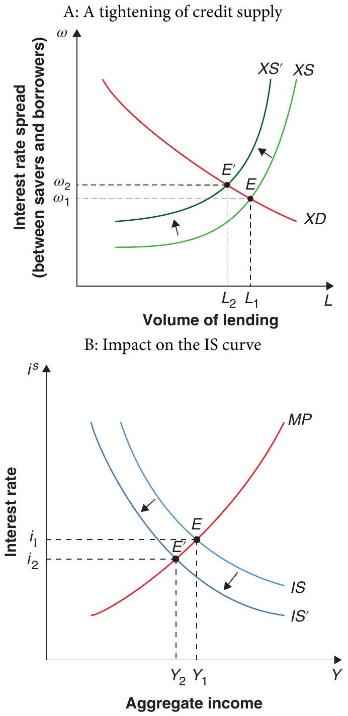
To introduce these new issues we can start from a simple IS-LM type of model, as in the lower panel of Figure 21.2.6
If there are financial intermediaries, there must be multiple interest rates - one that is paid to savers \(\left(i^{s}\right)\), and another that is charged from borrowers \(\left(i^{b}\right)\). Otherwise, of course, how would those intermediaries make any money? This market, depicting the supply of loans and the demand for loans, is shown in the upper panel of Figure 21.2. The IS curve below is drawn for a given level of spread.
As a result, the role of intermediation introduces a new channel for the amplification and propagation of economic shocks. For instance, suppose a high level of economic activity affects asset prices, and hence the net worth of financial intermediaries and borrowers. This will allow for additional borrowing at any level of spread (a shift of the XS curve to the right). This makes the IS curve flatter than what it would otherwise be: the same change in income would be associated with a smaller change in the interest rate paid to savers. This amplifies the effects on output of any shift in the LM/MP curves.
Even more interestingly, this lets us consider the effects of direct shocks to intermediation - beyond the amplification of other shocks. An upward shift of the XS curve (less credit available for any level of spread) means a downward shift to the IS curve - a larger equilibrium spread translated into less interest being paid to savers. This shock, illustrated in Figure 21.2, leads (in the absence of monetary policy compensating for the negative shock) to an output contraction with falling interest rates. Anything that impairs the capital of financial intermediaries (say, a collapse in the prices of mortgage-backed securities they hold) or that tighten leverage constraints (say, they are required to post more collateral when raising funds because the market is suspicious of their solvency) will correspond to such an upward shift of the XS curve. If the IS curve is shifted far enough to the left, monetary policy may be constrained by the zero lower bound on interest rates. Does all of that sound familiar?
Needless to say, a simple IS-LM type of framework leaves all sorts of questions open in terms of the microfoundations behind the curves we’ve been fiddling around with. To that point we now turn.
21.2.2 A model of quantitative easing
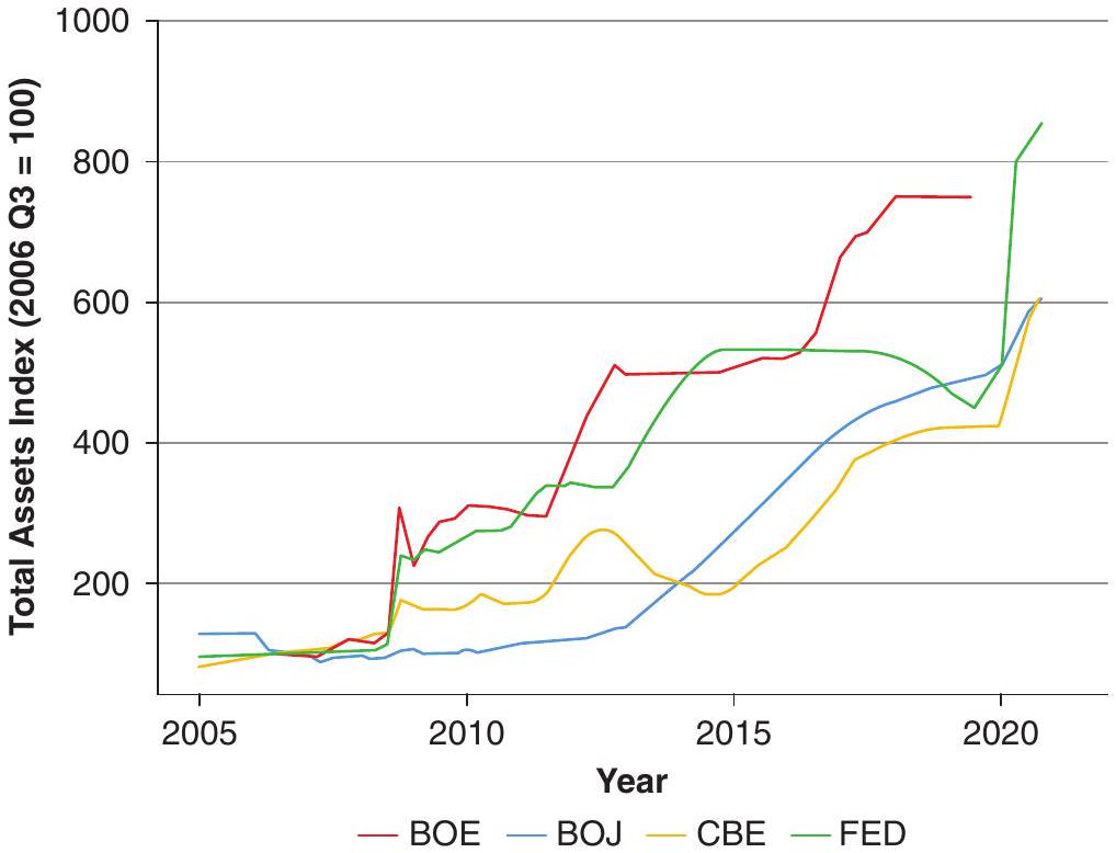
Now we focus on the role of the central bank balance and, more specifically, on the role of central bank reserves in the conduct of unconventional monetary policy. This emphasis has a practical motivation. As Figure 21.3 makes clear, the Federal Reserve (and other central banks) have issued reserves to purchase government bonds, private-sector bonds and other kinds of papers, dramatically enlarging the size of central bank balance sheets.
The assets in Figure 21.3 have been financed mostly with overnight interest paying voluntarily held deposits by financial institutions at the central bank. We call these deposits reserves for short.
As Reis (2016) emphasises, reserves have two unique features that justify this focus. First, the central bank is the monopoly issuer of reserves. As a monopoly issuer, it can choose the interest to pay on these reserves. Second, only banks can hold reserves. This implies that the aggregate amount of reserves in the overall banking system is determined by the central bank.
The liability side of a central bank balance sheet has two main components: currency (think of it as bank notes) and reserves. Together, currency and reserves add up to the monetary base. The central bank perfectly controls their sum, even if it does not control the breakdown between the two components of the monetary base.
These two properties of the central bank imply that the central bank, can in principle, choose both the quantity of the monetary base and the nominal interest rate paid on reserves. Whether it can also control the quantity of reserves, and do so independently of the interest rate that it pays, depends on the demand for reserves by banks7.
Before the 2008 financial crisis, central banks typically adjusted the volume of reserves to influence nominal interest rates in interbank markets. The zero lower bound made this policy infeasible during the crisis. Post-crisis, many central banks adopted a new process for monetary policy: they set the interest rate on reserves, and maintained a high level of reserves by paying an interest rate that is close to market rates (on bonds, say). In turn, changes in the reserve rate quickly feed into changes in interbank and other short rates.
Let \(D_{t}\) be the real value of a central bank-issued means of payment. You can think of it as central bank reserves. But following Diba and Loisel (2020) and Piazzesi et al. (2019), you can also think of it as a digital currency issued by the monetary authority and held directly by households8. In either case, the key feature of \(D_{t}\) is that it provides liquidity services: it enables parties to engage in buying, selling, and settling of balances. In what follows, we will refer to \(D_{t}\) using the acronym MP (means of payment, not be confused with our earlier use of MP for monetary policy), but do keep in mind both feasible interpretations. Later in this chapter we will show that the model developed here can also be extended (or reinterpreted, really) to study a more conventional situation in which only commercial banks have access to accounts at the central bank and households only hold deposits at commercial banks.
The simplest way to model demand for MP is to include it in the utility function of the representative household:
\[ u_{t}=\left(\frac{\sigma}{\sigma-1}\right) Z_{t}^{\left(\frac{\sigma-1}{\sigma}\right)}, Z_{t}=C_{t}^{\alpha} D_{t}^{1-\alpha}, \tag{21.5}\]
where \(\sigma>0\) is the interemporal elasticity of substitution in consumption, and is a Cobb-Douglas weight with \(\alpha\) that lies between 0 and 1. The representative household maximises the present discounted value of this utility flow subject to the following budget constraint:
\[ \dot{D}_{t}+\dot{B}_{t}=Y_{t}+\left(i_{t}^{b}-\pi_{t}\right) B_{t}+\left(i_{t}^{d}-\pi_{t}\right) D_{t}-C_{t}, \tag{21.6}\]
where \(B_{t}\) is the real value of a nominal (currency-denominated) bond, issued either by the government or by the private sector, \(i_{t}^{b}\) is the nominal interest rate paid by the bond, and \(i_{t}^{d}\) is the nominal interest rate paid by the central bank to holders of \(D_{t}\). (Income \(Y_{t}\) comprises household income and government transfers.) In accordance with our discussion above, the monetary authority controls this interest rate and the supply of MP9.
Since we do not want to go into the supply side of the model in any detail here, we simply include a generic formulation of household income, which should include wage income but could have other components as well. Government transfers must be included because governments may wish to rebate to agents any seigniorage collected from currency holders.
Let total assets be \(A_{t}=B_{t}+D_{t}\). Then we can write the budget constraint as
\[ \dot{A}_{t}=Y_{t}+\left(i_{t}^{b}-\pi_{t}\right) A_{t}-\left(i_{t}^{b}-i_{t}^{d}\right) D_{t}-C_{t} . \tag{21.7}\]
In the household’s optimisation problem, \(A_{t}\) is a state variable and \(D_{t}\) and \(C_{t}\) are the control variables. First order conditions are
\[ \alpha Z_{t}^{\left(\frac{\sigma-1}{\sigma}\right)}=C_{t} \lambda_{t} \tag{21.8}\]
\[ (1-\alpha) Z_{t}^{\left(\frac{\sigma-1}{\sigma}\right)}=\lambda_{t} D_{t}\left(i_{t}^{b}-i_{t}^{d}\right) \tag{21.9}\]
\[ \dot{\lambda}_{t}=-\lambda_{t}\left(i_{t}^{b}-\pi_{t}-\rho\right), \tag{21.10}\]
where \(\lambda_{t}\) is the shadow value of household assets (the co-state variable in the optimisation problem). These conditions are standard for the Ramsey problem, augmented here by the presence of the MP. It follows from (21.8) and (21.9) in logs, denoted by small case letters, the demand function for MP is
\[ d_{t}=c_{t}-\Delta_{t}, \tag{21.11}\]
where
\[ \Delta_{t}=\log \left[\left(\frac{\alpha}{1-\alpha}\right)\left(i_{t}^{b}-i_{t}^{d}\right)\right] . \tag{21.12}\]
So, intuitively, demand for MP is proportional to consumption and decreasing in the opportunity cost \(\left(i_{t}^{b}-i_{t}^{d}\right)\) of holding MP. Notice that this demand function does not involve satiation: as \(i_{t}^{b}-i_{t}^{d}\) goes to zero, \(d_{t}\) does not remain bounded. From a technical point of view, it means that we cannot consider here a policy of \(i_{t}^{d}=i_{t}^{b}\)10.
The appendix shows that in logs, the Euler equation is
\[ \dot{c}_{t}=\sigma\left(i_{t}^{b}-\pi_{t}-\rho\right)+(1-\sigma)(1-\alpha) \dot{\Delta}_{t} . \tag{21.13}\]
Differentiating (21.11) with respect to time yields
\[ \dot{c}_{t}-\dot{d}_{t}=\dot{\Delta}_{t} . \tag{21.14}\]
To close the model we need two more equations. One is the law of motion for real MP holdings, also in logs:
\[ \dot{d}_{t}=\mu-\pi_{t}, \tag{21.15}\]
where \(\mu\) is the rate of growth of the nominal stock of MP. Intuitively, the real stock rises with \(\mu\) and falls with \(\pi\). So \(\mu\) and \(i_{t}^{d}\) are the two policy levers, with \(i_{t}^{b}\) endogenous (market-determined).
From (21.14) and (21.15) it follows that
\[ \dot{c}_{t}=\mu-\pi_{t}+\dot{\Delta}_{t} . \tag{21.16}\]
This equation and the Euler equation (21.13) can be combined to yield
\[ \dot{\Delta}_{t}=\frac{\sigma\left(i_{t}^{b}-\rho\right)-\mu+(1-\sigma) \pi_{t}}{\alpha+\sigma(1-\alpha)} . \tag{21.17}\]
Now, given the definition of \(\Delta_{t}\) in (21.12),
\[ i_{t}^{b}=\left(\alpha^{-1}-1\right) e^{\Delta_{t}}+i_{t}^{d}, \tag{21.18}\]
which can trivially be included in (21.17)
\[ \dot{\Delta}_{t}=\frac{\sigma\left[\left(\alpha^{-1}-1\right) e^{\Delta_{t}}+i_{t}^{d}-\rho\right]-\mu+(1-\sigma) \pi_{t}}{\alpha+\sigma(1-\alpha)} . \tag{21.19}\]
Recall next that because the economy is closed all output is consumed, so \(c_{t}=y_{t}\). If we again define \(x_{t} \equiv y_{t}-\bar{y}\) as the output gap, the Euler equation becomes
\[ \dot{x}_{t}=\sigma\left(i_{t}^{b}-\pi_{t}-r^{n}\right)+(1-\sigma)(1-\alpha) \dot{\Delta}_{t}, \tag{21.20}\]
where, as in previous sections, the natural rate of interest is \(r^{n} \equiv \rho+\sigma^{1} g\), and \(g\) is the exogenous rate of growth of the natural rate of output \(\bar{y}\).
Next, with \(c_{t}=y_{t}\) the MP demand function (21.11) becomes
\[ d_{t}=y_{t}-\Delta_{t}, \tag{21.21}\]
which, in deviations from steady state, is
\[ x_{t}=\left(d_{t}-\bar{d}\right)+\left(\Delta_{t}-\bar{\Delta}\right) . \tag{21.22}\]
We close the model with the Phillips curve, using the same formulation as in this chapter and earlier:
\[ \dot{\pi}_{t}=\rho \pi_{t}-\kappa x_{t} . \tag{21.23}\]
Replacing (21.22) in (21.23) we get
\[ \dot{\pi}_{t}=\rho \pi_{t}-\kappa\left(d_{t}-\bar{d}\right)-\kappa\left(\Delta_{t}-\bar{\Delta}\right) . \tag{21.24}\]
That completes the model, which can be reduced to a system of three differential equations in 3 unknowns, \(\pi_{t}, d_{t}\) and \(\Delta_{t}\), whose general solution is quite complex. But there is one case, that of log utility, which lends itself to a simple and purely graphical solution. On that case we focus next.
If \(\sigma=1\), then (21.19) simplifies to:
\[ \dot{\Delta}_{t}=\left(\alpha^{-1}-1\right) e^{\Delta_{t}}+i_{t}^{d}-\rho-\mu . \tag{21.25}\]
This is an unstable differential equation in \(\Delta_{t}\) and exogenous parameters or policy variables. Thus, when there is a permanent shock, \(\Delta_{t}\) jumps to the steady state. This equation does not depend on other endogenous variables \(\left(x_{t}, d_{t}, \pi_{t}\right.\) or \(\left.i_{t}^{b}\right)\), so it can be solved separately from the rest of the model. The evolution over time of \(\Delta_{t}\) depends on itself and the policy parameters \(i_{t}^{d}\) and \(\mu\)11.
Now the Phillips curve and the law of motion for MP are a system of two differential equations in two unknowns, \(\pi_{t}\) and \(d_{t}\), with \(\left(\Delta_{t}-\bar{\Delta}\right)\) exogenously given. In matrix form the system is
\[ \left[\begin{array}{c} \dot{r}_{t} \\ \dot{d}_{t} \end{array}\right]=\Omega\left[\begin{array}{l} \pi_{t} \\ d_{t} \end{array}\right]+\left[\begin{array}{c} \kappa \bar{d}-\kappa\left(\Delta_{t}-\bar{\Delta}\right) \\ \mu \end{array}\right], \tag{21.26}\]
where
\[ \Omega=\left[\begin{array}{cc} \rho & -\kappa \\ -1 & 0 \end{array}\right] . \tag{21.27}\]
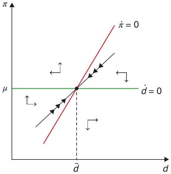
It is straightforward to see that \(\operatorname{Det}(\Omega)=-\kappa<0\), and \(\operatorname{Tr}(\Omega)=\rho>0\). It follows that one of the eigenvalues of \(\Omega\) is positive and the other is negative. Since \(\pi_{t}\) is a jumpy variable and \(d_{t}\) is a sticky or state variable, we conclude that the \(2 \times 2\) system is saddle-path stable, as seen in Figure 21.4.
Before considering the effects of shocks on the dynamics of this system, let us ask: why this model? What does it add to the standard NK formulation?
The first is realism. Since the Great Financial Crisis, many central banks have begun using the interest paid on reserves as an instrument of monetary policy. This policy alternative is not something one can study in conventional NK models.
Second, and more important, not only different interest rates, but the size and composition of the central bank’s balance sheet now matter. Changes in the speed of MP creation and open market operations involving MP can affect both inflation and output. For a more general discussion of the role of the central bank’s balance sheet, see Curdia and Woodford (2011).
Third, a technical but policy-relevant point: this model does not suffer from the problem of nonuniqueness of equilibrium that plagues NK models with an exogenous nominal interest rate, as we saw in Chapter 15. For further discussion, see Hall and Reis (2016) and Diba and Loisel (2020).
21.2.3 Effects of monetary policy shocks
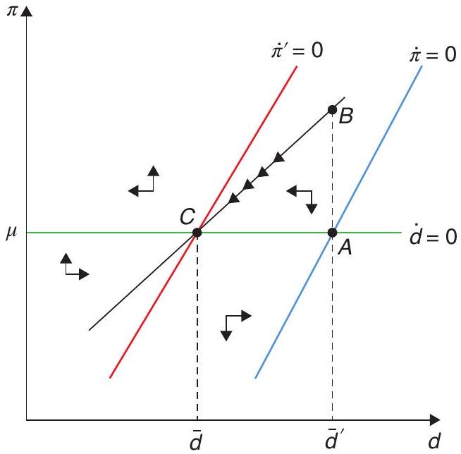
Consider first the effects of an unexpected and permanent reduction in \(i_{t}^{d}\), one of the two policy tools the central bank has. Suppose that at time \(0, i_{t}^{d}\) moves from \(i^{d}\) to \(\underline{i}^{d}\), where \(\underline{i}^{d}<i^{d}\). We show this in Figure 21.5.
Recall that in steady state the market rate of interest on bonds is pinned down by \(i^{b}=\rho+\mu\). So, as \(i_{t}^{d}\) falls, \(\bar{\Delta}\), the steady state gap between the two interest rates rises. We saw that in response to a permanent policy shock, \(\Delta_{t}\) will immediately jump to its new (higher, in this case) steady state level. This means that we can look at the dynamics of \(\pi_{t}\) and \(d_{t}\) independently of \(\Delta_{t}\).
The other thing to notice is that as the steady state gap \(\left(i^{b}-i^{d}\right)\) goes up, steady state demand for MP falls. In the phase diagram in Figure 21.5, this is reflected in the fact that the \(\dot{\pi}=0\) schedule moves to the left, and the new steady state is at point \(C\). On impact, the system jumps up to point \(B\), with inflation temporarily high. Thereafter, both inflation and real stocks of MP fall toward their new steady state levels.
What happens to consumption and output? The cut in \(i_{t}^{d}\) makes people want to hold less MP, but the stock of MP cannot fall immediately. What equilibrates the market for MP is a an upward jump in consumption (and output, given that prices are sticky). The temporary boom causes an increase in inflation above the rate \(\mu\) of nominal MP growth, which over time erodes the real value of the stock of MP outstanding, until the system settles onto its new steady state.
In summary: the permanent cut in the interest rate paid on MP causes a temporary boom. Inflation rises and then gradually falls and so does output. All of this happens without modifying the pace of nominal MP growth. So, changes in the interest rate paid on central bank reserves (or on a digital means of payment) do serve as tool of monetary policy, with real effects.
Consider next the effects of an unexpected and permanent increase in \(\mu\), the other tool the central bank has at its disposal. Suppose that at time 0 , policy moves from \(\mu\) to \(\bar{\mu}\), where \(\bar{\mu}>\mu\). Recall again that in steady state the market rate of interest on bonds is pinned down by \(i^{b}=\rho+\mu\). So, as \(\mu\) rises and \(i^{d}\) remains constant, \(\bar{\Delta}\), the steady state gap between the two interest rates will go up. But \(\Delta_{t}\) will jump right away to \(\bar{\Delta}\), so again we can look at the dynamics of the 2 × 2 system independently of \(\Delta_{t}\).
As the steady state gap \(\left(i^{b}-i^{d}\right)\) rises, steady state demand for MP goes down. In the phase diagram in Figure 21.6, this is reflected in the fact that the \(\dot{\pi}=0\) schedule moves to the left. But now the \(\dot{d}=0\) schedule also shifts (upward), so that the new steady state is at point \(F\). On impact, the system jumps up to point \(E\), with inflation overshooting its new, higher, steady state level. Thereafter, both inflation and the real stock of MP fall toward their new steady state levels.
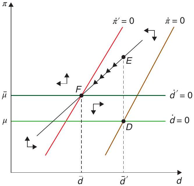
Note that the overshoot is necessary to erode the real value of MP, since in the new steady state agents will demand less of it. As in the previous case, inflation rises since consumption and output are temporarily above their steady state levels.
Finally, consider the effects of a temporary drop in \(i_{t}^{d}\), the interest rate paid on MP. To fix ideas, consider the following unexpected shock occurring at time 0:
\[ i_{t}^{d}=\left\{\begin{array}{clc} \underline{i}^{d}<i^{d} & \text { for } & 0 \leq t<T \\ i^{d} & \text { for } & t \geq T \end{array}\right. \tag{21.28}\]
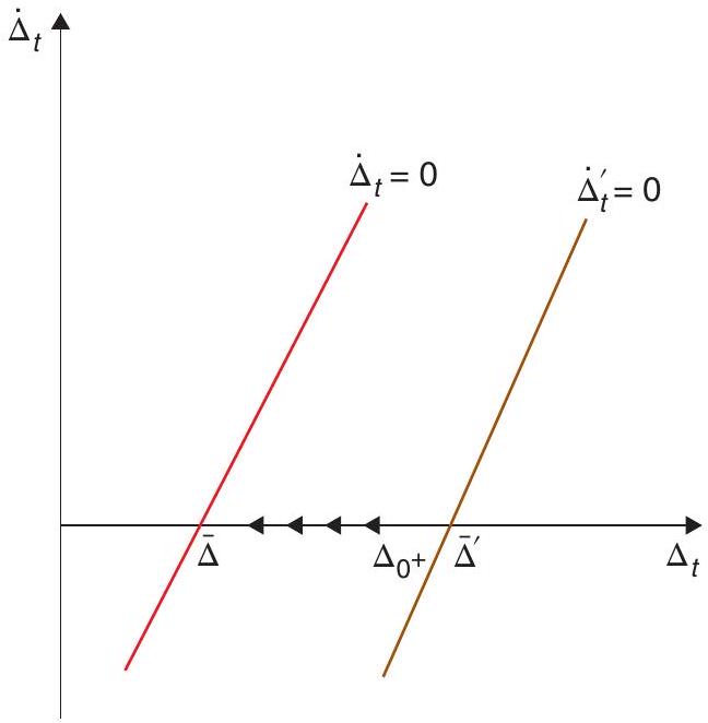
To sort out what happens it helps to begin by asking what is the trajectory of \(\Delta_{t}\). It rises on impact, but it does not go all the way up to \(\bar{\Delta}^{\prime}\), the level it would take on if the change were permanent. The differential \(\Delta_{t}\) falls thereafter, so that it can jump at \(T\) when \(i_{t}^{d}\) goes back to its initial level, ensuring that \(\Delta_{t}\) is back to its initial steady state level \(\bar{\Delta}\) an instant after \(T\) (in contrast to the policy variable, \(i^{b}\) cannot jump).
Let \(\Delta_{0^{+}}\)be the value of \(\Delta_{t}\) once the unexpected shock happens at \(t=0\). It must be the case, by the arguments above, that \(\bar{\Delta}<\Delta_{0}+<\bar{\Delta}^{\prime}\). You can see this evolution in the phase diagram in Figure 21.7, where we show the (linearised version of) the \(\dot{\Delta}_{t}=0\) schedule.
What are the implications for the dynamic behaviour of inflation and the real stock of MP? We can study that graphically in Figure 21.8 below. If the policy change were permanent, the \(\dot{\pi}=0\) schedule would have moved all the way to \(\dot{\pi}^{\prime \prime}=0\), giving rise to a steady state at \(H\). But the fact that \(\Delta_{0}-\bar{\Delta}^{\prime}<0\) offsets some of that leftward movement. So, the \(\dot{\pi}=0\) schedule moves to \(\dot{\pi}^{\prime}=0\), creating a temporary (for an instant) steady state at \(G\).
Ask what would happen if \(\Delta_{t}\) were to remain at \(\Delta_{0}\) until time \(T\). Inflation would jump up on impact. But it cannot go beyond point \(K\), because if it did the system would diverge to the northwest afterwards. So, inflation would jump to a point like \(N\). After the jump, the economy would begin to move following the arrows that correspond to the system with steady state at \(G\).
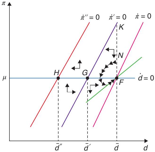
Of course, an instant after \(T\), and because of the movement in \(\Delta_{t}\), the locus \(\dot{\pi}^{\prime}=0\) begins to shift to the right. But this does not affect the qualitative nature of the adjustment path, because the system always lies to the right of the shifting \(\dot{\pi}^{\prime}=0\) locus, and thus obeys the same laws of motion as it did an instant earlier. The evolution of inflation and real MP is guided by the need that, at \(T\), the system must be on the saddle path leading to the initial steady state at point \(F\).
You can see from the phase diagram that after the initial jump up, inflation falls between times 0 and \(T\), and rises thereafter. The real value of MP drops initially due to the high inflation, but then gradually recovers as \(\pi_{t}\) falls below \(\mu\). One can show also that output goes through a boom between times 0 and \(T\), takes a discrete drop at \(T\) when the interest rate \(i_{t}^{d}\) rises again, and recovers gradually until returning to its initial steady state level.
21.3 Policy implications and extensions
21.3.1 Quantitative easing
We emphasised above that in this model the monetary authority has access to two policy levers: an interest rate \(\left(i^{d}\right)\) and a quantity tool \((\mu)\)-or potentially, two interest rates, if the central bank chooses to engage in open market operations and use changes in quantities to target \(i^{b}\). So we have gone beyond the realm of conventional policy, in which control of the single interest rate on bonds is the only alternative.12
We saw earlier that a dilemma arises when the nominal interest rate is against the zero lower bound. Can we use the model we have just built to study that conundrum? Is there a policy that can stabilise output and inflation when the lower bound binds? The answer is yes (subject to parameter values), and in what follows we explain how and why.
To fix ideas, let us go back to the situation studied earlier in this chapter, in which, because of lagging productivity growth, the natural rate of interest drops. Suppose initially \(i^{b}=r^{n}>0, i_{t}^{d}=0\)
and \(\mu=\pi=0\). Then the following shock hits
\[ r_{t}^{n}=\left\{\begin{array}{lll} \underline{r}^{n}<0 & \text { for } & 0 \leq t<T \\ r^{n}>0 & \text { for } & t \geq T . \end{array}\right. \tag{21.29}\]
So starting from \(r^{n}\), at time 0 the natural rate of interest unexpectedly drops down to \(\underline{r}^{n}<0\) and it remains there until time \(T\), when it returns to \(r^{n}\) and stays there forever.
Notice first that if \(\sigma=1\), during the duration of the shock the NKIS curve (21.20) becomes:
\[ \dot{x}_{t}=\left(i_{t}^{b}-\pi_{t}-\underline{r}^{n}\right) \tag{21.30}\]
So \(\dot{x}_{t}=\pi_{t}=0\) would require \(i_{t}^{b}=\underline{r}^{n}<0\). But this is impossible if the zero lower bound is binding and hence \(i_{t}^{b}\) must be non-negative. Our first conclusion, therefore, is that for monetary policy to get around the zero lower bound problem we must focus on the case in which \(\sigma \neq 1\). This is the case in which the utility function is not separable in consumption and liquidity (MP), so that that changes in the opportunity cost of holding liquidity have an impact on the time profile of consumption and aggregate demand.
If we go back to the case in which \(\sigma \neq 1\), during the duration of shock the NKIS curve (21.20) becomes:
\[ \dot{x}_{t}=\sigma\left(i_{t}^{b}-\pi_{t}-\underline{r}^{n}\right)+(1-\sigma)(1-\alpha) \dot{\Delta}_{t} \tag{21.31}\]
It follows from (21.31) that \(\dot{x}_{t}=x_{t}=0\) and \(\pi_{t}=0\) if and only if
\[ \dot{\Delta}_{t}=\frac{\sigma\left[\left(\alpha^{-1}-1\right) e^{\Delta_{t}}+i_{t}^{d}-\underline{r}^{n}\right]}{(\sigma-1)(1-\alpha)} . \tag{21.32}\]
where we have used \(i_{t}^{b}=\left(\alpha^{-1}-1\right) e^{\Delta_{t}}+i_{t}^{d}\). For simplicity, focus on the case \(\sigma>1\). In that case, the RHS of this equation is positive (recall \(\underline{r}^{n}<0\) ), so the interest gap \(\Delta_{t}\) must rise gradually during the period of the shock.
At this point we have to take a stance on a difficult question: does the zero lower bound apply to \(i_{t}^{d}\) as well? If we interpret \(d_{t}\) narrowly, as reserves commercial banks hold at the central bank, the answer may be negative: it is not hard to think of liquidity or safety reasons why banks would want to hold reserves at the central bank even if they have to pay a cost to do so. But if we interpret \(i_{t}^{d}\) more broadly as a digital currency, then the answer could be yes, because if the nominal interest rate on reserves is negative, households could prefer to hold their liquidity under the mattress and look for substitutes as a means of payment. This is the standard “disintermediation” argument for the zero lower bound. To avoid wading into this controversy, in this section we assume \(i_{t}^{d} \geq 0\).
Moreover, and to keep things very simple, we assume the central bank keeps \(i_{t}^{d}\) at its steady state level of zero throughout. In that case, the equation for the evolution of \(\Delta_{t}(21.32)\) reduces to
\[ \dot{\Delta}_{t}=\frac{\sigma\left[\left(\alpha^{-1}-1\right) e^{\Delta_{t}}-\underline{r}^{n}\right]}{(\sigma-1)(1-\alpha)} . \tag{21.33}\]
Next, recall the liquidity demand function \(d_{t}=c_{t}-\Delta_{t}\), which implies that if consumption is to be constant during the period of the shock, then \(\dot{d}_{t}=-\dot{\Delta}_{t}\) That is to say, the interest gap can be rising only if the (real) stock of MP is falling. But since we are also requiring zero inflation during that period, real MP decline is the same as nominal MP decline, implying \(\mu_{t}=-\dot{\Delta}_{t}<0\).
So now we know what the time profile of \(\Delta_{t}\) and \(d_{t}\) must be between times 0 and \(T\). What about the initial and terminal conditions? Suppose we require \(i_{T}^{b}=r^{n}\), so that the interest rate on bonds will
be exactly at its steady state level at time T. Since \(i_{t}^{d}\) is constant at zero and \(\Delta_{t}\) must be falling, it follows that \(i_{t}^{b}\) must be rising during the length of the shock. So \(i_{t}^{b}\) must have jumped down at time 0 , which in turn means \(d_{t}\) must have jumped up at the same time.
In summary: if \(\sigma>1\), a policy that keeps output at “full employment” and inflation at zero, in spite of the shock to the natural interest rate, involves: a) discretely increasing the nominal and real stock of MP at the time of the shock, causing the interest rate on bonds to fall on impact in response to the shock, in what resembles QE;13 b) allowing the nominal and real stock of MP to fall gradually during the period of the shock, in what resembles the “unwinding” of QE; c) once the shock is over, ensuring policy variables return to (or remain at) their steady state settings: \(\mu=0\) and \(i_{t}^{d}=0\) for all \(t \geq T\).14
The intuition for why this policy can keep the economy at full employment is as follows. With two goods (in this case, consumption and liquidity services) entering the utility function, what matters for the optimal intertemporal profile of expenditure is not simply the real interest rate in units of consumption, but in units of the bundle \(Z_{t}\) that includes both the consumption good and the real value of MP. Because the nominal rate on bonds cannot fall below zero, what brings the real “utility-based” interest rate down to the full employment level is the behaviour of the “relative price” \(\Delta_{t}\). When \(\sigma>1\), \(\Delta_{t}\) has to rise to achieve the desired effect. If, on the contrary, we assumed \(\sigma<1\), then \(\Delta_{t}\) would have to fall over time the period of the shock.15
In the case \(\sigma>1\), the gradual increase in \(\Delta_{t}\) follows an initial drop in the same variable, caused by a discrete increase in the nominal and real stock of MP. This “quantitative easing”, if feasible, manages to keep the economy at full employment and zero inflation in spite of the shock to the natural rate of interest and the existence of a zero lower bound for both nominal interest rates.
21.3.2 Money and banking
An objection to the arguments so far in this chapter is that digital currencies do not yet exist, so households do not have accounts at the central bank. In today’s world, the only users of central bank reserves are commercial banks. But most households do use bank deposits for transactions.
This does not mean that our previous analysis is useless. On the contrary, with relatively small modifications, it is straightforward to introduce a banking system into the model. Piazzesi et al. (2019) carry out the complete analysis. Here, we just sketch the main building blocks.
A simplified commercial bank balance sheet has deposits and bank equity on the liability side, and central bank reserves and other assets (loans to firms, government bonds) on the asset side. Banks are typically borrowing-constrained: they can issue deposits only if they have enough collateral - where central bank reserves and government bonds are good collateral.
So now \(d_{t}\) can stand for (the log of) the real value of deposits held in the representative commercial bank, and \(i_{t}^{d}\) is the interest rate paid on those deposits. Because deposits provide liquidity services, \(i_{t}^{d}\) can be smaller than the interest rate on bonds, \(i_{t}^{b}\).
The central bank does not control \(i_{t}^{b}\) or \(i_{t}^{d}\) directly. But banks do keep reserves at the central bank, and this gives the monetary authority indirect control over market rates. Denote by \(i_{t}^{h}\) the interest rate paid on central bank reserves. It is straightforward to show (see Piazzesi et al. (2019) for details) that optimal behaviour by banks leads to
\[ \left(i_{t}^{b}-i_{t}^{d}\right)=\ell\left(i_{t}^{b}-i_{t}^{h}\right), \tag{21.34}\]
where \(\ell<1\) if banks are borrowing-constrained and/or have monopoly power.16 Whenever \(\ell<1\), \(\left(i_{t}^{b}-i_{t}^{h}\right)(1-\ell)=i_{t}^{d}-i_{t}^{h}>0\) so that the rate on deposits and on central bank reserves are linked, with
the former always above the latter. The central bank can affect the rate on deposits by adjusting both the quantity of reserves and the interest rate paid on them. Demand for deposits, as in the previous subsection, depends on the opportunity cost of holding deposits:
\[ d_{t}=c_{t}-\log \left[\left(\frac{\alpha}{1-\alpha}\right)\left(i_{t}^{b}-i_{t}^{d}\right)\right] . \tag{21.35}\]
Using the equation above we have
\[ d_{t}=c_{t}-\log \left[\left(\frac{\alpha}{1-\alpha}\right) \ell\left(i_{t}^{b}-i_{t}^{h}\right)\right]=c_{t}-\log \left[\left(\frac{\alpha}{1-\alpha}\right) \ell\right]-\log \left(i_{t}^{b}-i_{t}^{h}\right) . \tag{21.36}\]
With this expression in conjunction with the dynamic NKIS curve, the NKPC, and the corresponding policy rules, we have a macro model almost identical to that of the earlier sections, and which can be used to analyse the effects of exogenous shocks and policy changes.
Aside from realism, this extended version has one other advantage: shocks to financial conditions can now become another source of business cycle variation that needs to be counteracted by monetary (and perhaps fiscal) policy. The parameter \(\ell\), reflecting conditions in the financial markets, the quality of the collateral, the extent of competition, etc., enter as shifters in the expression for deposit demand. To fix ideas, consider what happens if we continue with the policy arrangement of the previous subsection, with \(i_{t}^{b}=0\) and the interest rate on reserves (now labelled \(i_{t}^{h}\) ) exogenously given. Then, and since \(d_{t}\) is a sticky variable that cannot jump in response to shocks, an unexpected change in \(\ell\) would imply a change in consumption, and, therefore, in aggregate demand and output. So, in the presence of shocks to financial market conditions, monetary policymakers have to consider whether and how they want to respond to such shocks.
21.3.3 Credit easing
So far the focus of this chapter has been on unconventional policies that involve changing the quantity of reserves by having the central bank carry out open market operations involving safe assets like government bonds. But at the zero lower bound, and if the interest rate on reserves is brought down to the level of the interest rate on bonds (a case of liquidity satiation, not considered above), then from the point of view of the private sector (of a commercial bank, say), central bank reserves and short-term, liquid government bonds become identical: they are both i.o.u’s issued by the state (or the consolidated government, if you wish), paying the same rate of interest. So, operations that involve swapping one for the other cannot have any real effects.
That is why, in the face of financial markets frictions and distortions, over the last decade and particularly since the Great Financial Crisis, central banks have turned to issuing reserves to purchase other kinds of assets, from corporate bonds to loans on banks’ balance sheets, in effect lending directly to the private sector. As mentioned at the outset, these are usually labelled credit easing policies, in contrast to the “quantitative easing” policies that only involve conventional open market operations.
Credit easing can be incorporated into a simple model like the one we have been studying in this chapter, or also into more sophisticated models such as those of Curdia and Woodford (2011) and Piazzesi et al. (2019). There are many obvious reasons why such policies can have real effects: one is that they can get credit flowing again when the pipes of the financial system become clogged or frozen in a crisis.
A related reason is that in this context policy can not only address aggregate demand shortfalls, but also help alleviate supply constraints - if, for instance, lack of credit keeps firms from having the necessary working capital to operate at the optimal levels of output. This all begs the question of what
policy rules ought to look like in such circumstances, a fascinating subject we cannot address here, but about which there is a growing literature - beginning with the 2009 lecture at LSE in which Ben Bernanke, then Fed Chair, explained the Fed’s approach to fighting the crisis, which stressed credit easing policies (Bernanke (2009).
21.4 Appendix
The FOC, (21.8)-(21.10) repeated here for convenience, are
\[ \alpha Z_{t}^{\left(\frac{\sigma-1}{\sigma}\right)}=C_{t} \lambda_{t} \tag{21.37}\]
\[ (1-\alpha) Z_{t}^{\left(\frac{\sigma-1}{\sigma}\right)}=\lambda_{t} D_{t}\left(i_{t}^{b}-i_{t}^{d}\right) \tag{21.38}\]
\[ \dot{\lambda}_{t}=-\lambda_{t}\left(i_{t}^{b}-\pi_{t}-\rho\right), \tag{21.39}\]
where we have defined
\[ C_{t}^{a} D_{t}^{1-\alpha} \equiv Z_{t} . \tag{21.40}\]
Combining the first two, we have demand for MP:
\[ D_{t}=\frac{C_{t}}{\left(\frac{\alpha}{1-\alpha}\right)\left(i_{t}^{b}-i_{t}^{d}\right)}, \tag{21.41}\]
which in logs is
\[ d_{t}=c_{t}-\Delta_{t}, \tag{21.42}\]
where
\[ \Delta_{t}=\log \left[\left(\frac{\alpha}{1-\alpha}\right)\left(i_{t}^{b}-i_{t}^{d}\right)\right] . \tag{21.43}\]
Next, differentiating (21.38) with respect to time and then combining with (21.40) yields
\[ \left(\frac{\sigma-1}{\sigma}\right) \frac{\dot{Z}_{t}}{Z_{t}}=\frac{\dot{C}_{t}}{C_{t}}-\left(i_{t}^{b}-\pi_{t}-\rho\right) . \tag{21.44}\]
Or, in logs
\[ \left(\frac{\sigma-1}{\sigma}\right) \dot{z}_{t}=\dot{c}_{t}-\left(i_{t}^{b}-\pi_{t}-\rho\right) . \tag{21.45}\]
Using demand for MP from (21.42) in the definition of \(Z_{t}\) (21.41) yields
\[ Z_{t}=C_{t}^{\alpha} D_{t}^{1-\alpha}=C_{t}\left(\frac{\alpha}{1-\alpha}\right)^{-(1-\alpha)}\left(i_{t}^{b}-i_{t}^{d}\right)^{-(1-\alpha)} . \tag{21.46}\]
Or, in logs
\[ z_{t}=c_{t}-(1-\alpha) \Delta_{t} . \tag{21.47}\]
Differentiating (21.48) with respect to time yields
\[ \dot{z}_{t}=\dot{c}_{t}-(1-\alpha) \dot{\Delta}_{t} . \tag{21.48}\]
Replacing the expression for \(\dot{z}_{t}\) from (21.46) in (21.49) we obtain the Euler equation (21.13) used in the text:
\[ \dot{c}_{t}=\sigma\left(i_{t}^{b}-\pi_{t}-\rho\right)+(1-\sigma)(1-\alpha) \dot{\Delta}_{t}, \tag{21.49}\]
which can be also written, perhaps more intuitively, as
\[ \dot{c}_{t}=\sigma\left[i_{t}^{b}-\pi_{t}-\left(\frac{\sigma-1}{\sigma}\right)(1-\alpha) \dot{\Delta}_{t}-\rho\right] . \tag{21.50}\]
This way of writing it emphasises that the relevant real interest rate now includes the term \(\left(\frac{\sigma-1}{\sigma}\right)(1-\alpha) \dot{\Delta}_{t}\), which corrects for changes in the relative price of the two items that enter the consumption function.
branch of government - the Treasury. The issuer is the same, and therefore these securities ought to have the same (or very similar) risk characteristics. If they also pay the same interest rate, then they become perfect substitutes in the portfolios of private agents. An operation involving exchanging reserves for bonds, or vice-versa, would have no reason to deliver real effects. A Modigliani-Miller irrelevance result would kick. However, there may be some special circumstances (fiscal or financial crisis, for instance) in which this equivalence breaks down. See the discussion in Reis (2016).
References
Beckworth, D. (2019). Facts, fears, and functionality of NGDP level targeting: A guide to a popular framework for monetary policy. Mercatus Research Paper.
Bernanke, B. S. (2009). The crisis and the policy response. Stamp Lecture, London School of Economics, January, 13, 2009.
Blanchard, O. & Galí, J. (2007). Real wage rigidities and the New Keynesian model. Journal of Money, Credit and Banking, 39, 35-65.
Brunnermeier, M., Eisenbach, T., & Sannikov, Y. (2013). Macroeconomics with financial frictions: A survey. Advances in Economics and Econometrics.
Calvo, G. A. (1978). On the time consistency of optimal policy in a monetary economy. Econometrica, 1411-1428.
Calvo, G. A. (1983). Staggered prices in a utility-maximizing framework. Journal of Monetary Economics, 12(3), 383-398.
Calvo, G. A. & Végh, C. A. (1996). Disinflation and interest-bearing money. The Economic Journal, 106(439), 1546-1563.
Curdia, V. & Woodford, M. (2011). The central-bank balance sheet as an instrument of monetarypolicy. Journal of Monetary Economics, 58(1), 54-79.
Diba, B. & Loisel, O. (2020). Pegging the interest rate on bank reserves: A resolution of New Keynesian puzzles and paradoxes. Journal of Monetary Economics.
Dornbusch, R. (1983). Real interest rates, home goods, and optimal external borrowing. Journal of Political Economy, 91(1), 141-153.
Eggertsson, G. B. & Woodford, M. (2003). Zero bound on interest rates and optimal monetary policy. Brookings Papers on Economic Activity, 2003(1), 139-233.
Eggertsson, G. B. & Woodford, M. (2004). Policy options in a liquidity trap. American Economic Review, 94(2), 76-79.
Gertler, M. & Karadi, P. (2011). A model of unconventional monetary policy. Journal of Monetary Economics, 58(1), 17-34.
Hall, R. E. & Reis, R. (2016). Achieving price stability by manipulating the central bank’s payment on reserves. National Bureau of Economic Research.
Hicks, J. R. (1937). Mr. Keynes and the “classics”; A suggested interpretation. Econometrica, 147-159.
Krugman, P. (1998). Japan’s trap. http://web.mit.edu/krugman/www/japtrap.html.
Kydland, F. E. & Prescott, E. C. (1977). Rules rather than discretion: The inconsistency of optimal plans. Journal of Political Economy, 85(3), 473-491.
Piazzesi, M., Rogers, C., & Schneider, M. (2019). Money and banking in a New Keynesian model. Working Paper, Stanford.
Reis, R. (2016). Funding quantitative easing to target inflation. LSE Research Online, http://eprints.lse.ac.uk/67883/.
Rogoff, K. (2017). Dealing with monetary paralysis at the zero bound. Journal of Economic Perspectives, 31(3), 47-66.
Summers, L. H. (2018). Secular stagnation and macroeconomic policy. IMF Economic Review, 66(2), 226-250.
Sumner, S. B. (2014). Nominal GDP targeting: A simple rule to improve Fed performance. Cato Journal. 34, 315.
Werning, I. (2011). Managing a liquidity trap: Monetary and fiscal policy. National Bureau of Economic Research.
Woodford, M. (2010). Financial intermediation and macroeconomic analysis. Journal of Economic Perspectives, 24(4), 21-44.
Woodford, M. (2016). Quantitative easing and financial stability. National Bureau of Economic Research. Working Paper 22285 http://www.nber.org/papers/w22285.
Woodford, M. (2020). Post-pandemic monetary policy and the effective lower bound.
On monetary policy during the pandemic, see Woodford (2020).↩︎
A good review of the discussion can be found in Rogoff (2017).↩︎
A technical clarification: in Chapter 15 we claimed that, in the absence of an activist interest rule, the canonical 2- equation New Keynesian model does not have a unique equilibrium. So why have no multiplicity issues cropped up in the analysis here? Because, to draw the phase diagram the way we did we assumed the central bank would do whatever it takes to keep \(\pi_{t}=x_{t}=0\) starting at \(T\) (including, perhaps, the adoption of an activist rule starting at that time). That is enough to pin down uniquely the evolution of the system before \(T_{j}\) because it must be exactly at the origin ( \(\pi_{t}=x_{t}=0\) ) at \(T\). See Werning (2011) for the formal details behind this argument.↩︎
Recall from Chapter 14 that \(\kappa \equiv \alpha^{2} \eta>0\), and \(\alpha^{-1}\) is the expected length of a price quotation in the Calvo (1983) model. So as prices become perfectly flexible, \(\kappa\) goes to infinity.↩︎
For details, see the discussion by Gertler on the paper by Eggertsson and Woodford (2003).↩︎
See Woodford (2010) from which this discussion is taken.↩︎
In particular, on whether banks’ demand for liquidity has been satiated or not. See the discussion in Reis (2016).↩︎
We will see later that, under some simple extensions, \(D_{t}\) can also be thought of as deposits issued by commercial banks. But let us stick with the digital currency interpretation for the time being.↩︎
You may be wondering where currency is in all of this. We have not modelled it explicitly, but we could as long as it is an imperfect substitute for MP (meaning they are both held in equilibrium even though they have different yields - zero in nominal terms in the case of currency).↩︎
According to Reis (2016), this is more or less what the Federal Reserve has tried to do since the Great Financial Crisis of 2007-09, thereby satiating the demand for liquidity.↩︎
This very helpful way of solving a model of this type is due to Calvo and Végh (1996).↩︎
Notice, however, that all the analysis so far (and what follows as well) assumes \(i^{d}<i^{b}\). That is, there is an opportunity cost of holding reserves (or MP, if you prefer) and therefore liquidity demand by banks (or households, again, if you prefer) is not satiated. The situation is different when the interest rate on reserves is the same as the interest rate on government bonds. Reserves are a liability issued by one branch of government - the central bank. Bonds or bills are a liability issued by another↩︎
QE involves issuing reserves to purchase bonds, and that is exactly what is going on here.↩︎
Notice this policy is not unique. There are other paths for MP and \(i_{t}^{d}\) that could keep output and inflation constant. We have just chosen a particularly simple one. Notice also that in the sequence we described, the interest gap \(\Delta_{t}\) jumps down on impact and then rises gradually until it reaches its steady level \(r^{n}>0\) at time \(T\), but this trajectory is feasible as long as the shock does not last too long ( \(T\) is not too large) and the shock is not too deep ( \(\underline{r}^{n}\) is not too negative). The constraints come from the fact that on impact \(\Delta_{t}\) drops but can never reach zero (because in that case demand for MP would become unbounded). In other words, the central bank is not free to pick any initial condition for \(\Delta_{t}\), in order to ensure that, given the speed with which it must rise, it will hit the right terminal condition at time \(T\). Part of the problem comes from the fact that we have assumed that the inflation rate in the initial steady state is zero, so the initial nominal interest rate on bonds is equal to the natural rate of interest. But, in practice, most central banks target inflation at 2 percent per year, which gives \(\Delta_{t}\) “more room” to drop, so that central bankers can freely engage in the kind of policy we have described. Moreover, in the aftermath of the 2007-09 global financial crisis there were suggestions to raise inflation targets higher, to give central banks even “more room” in case of trouble.↩︎
Dornbusch (1983) was the first to make this point.↩︎
By contrast, in the absence of financial frictions and with perfect competition, \(\ell=1\) and \(i_{t}^{d}=i_{t}^{h}\), so that the interest rate on deposits is equal to the rate paid on central bank reserves.↩︎