10 Unified growth theory
You will recall that among the key stylised facts we set out to explain in our study of economic growth was the very existence of growth in living standards: output per worker increases over time. This, however, has only been true for a very short span in human history, starting with the Industrial Revolution and the birth of modern economic growth.
For most of history, the prevailing situation was one that we may call Malthusian stagnation. In other words, there obviously were massive increases in productivity - the wheel, agriculture, domesticated animals, ships, double-entry bookkeeping - but these did not really translate into increased living standards, or into sustained productivity growth. Instead, as per the Malthusian assumption (recall our discussion of the Kremer (1993) paper in (Chapter 6), those increases in productivity mostly translated into increases in population.
Then at some point, around the 18th century, the Great Divergence happened (see Figure 10.1): a few Western European countries, and then the Western offshoots in the New World, took off and never looked back. They inaugurated the age of sustained economic growth, which eventually spread to most other countries around the world, and which has been the object of our study in this first part of the book.
But this begs the question: how did that transition happen? Is there any way in which we can understand within a single framework the growth process in the Malthusian and modern eras combined? Can we understand why the latter emerged in the first place, how, from stability, suddenly growth popped up?1 This is the object of unified growth theory, a somewhat grandiosely named attempt at understanding growth from the perspective of millennia. This chapter constitutes a brief introduction to these ideas, following the presentation in Galor (2005). The fact that it uses some features of the OLG model explains why we have this discussion now.
10.1 From Malthus to growth
Growth seems to have experienced a kink around the end of the 18th century, when it accelerated dramatically.
While we have argued above that technological progress and increases in productivity have been features of human history for millennia, it is pretty much undeniable that the pace at which such progress took place until the last couple of centuries was much, much slower than what we have come to expect in recent times. The slow pace of productivity increases, combined with the Malthusian effect of those increases on population growth, meant that output per worker (i.e. living standards) grew very slowly over this period. Put simply, whenever things got a little better, people would starve less, live a little longer, have more kids, more of whom would reach adult age, etc. We would then simply end up sharing the increased output among a larger number of people, with essentially the same amount going for each of these people as before things had gotten better. In other words, increases in income per capita were essentially temporary, and eventually dissipated. It may sound odd to us today, but these were times when parents and sons lived in the same world, and so did their children and grandchildren. Progress was just too slow to be noticeable.
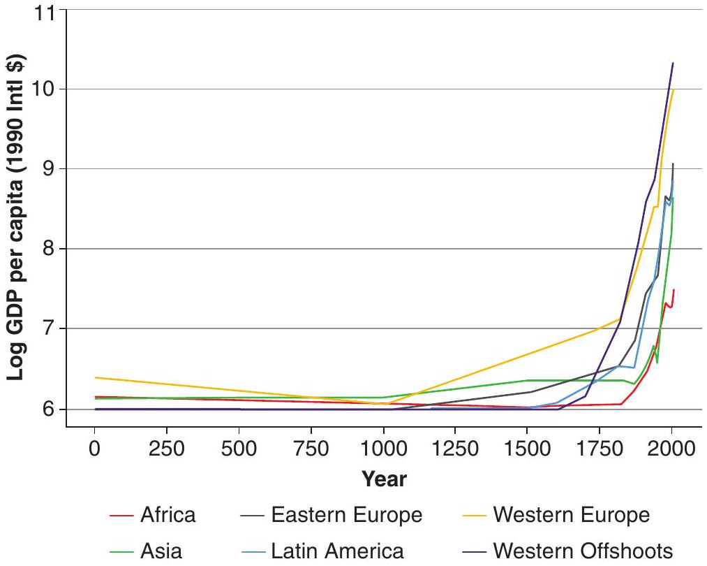
Mind you, stagnation doesn’t mean that these were boring times when nothing particularly interesting happened. Much to the contrary, hovering around subsistence level meant that negative productivity shocks (say, droughts) were devastating. The flipside of the adjustment described above would clearly hold: bad shocks would mean people dying early, fewer kids reaching adulthood, etc., bringing population down.
By the same token, there were substantial differences across countries and regions. Naturally, some places were more productive (fertile land, natural resources, location) and technology varied substantially. However, more productive countries or regions were not richer on a per capita basis - they just had more people, as in China or the Indian subcontinent. In sum, this scenario had a natural implication for cross-country comparisons: population (or more precisely, population density) is the right measure of development in this era.
As such, how do we know that, from a global perspective, technological progress and economic performance were rather unimpressive? Because global population growth was very slow over the period, according to the best historical and archaeological evidence.
10.1.1 The post-Malthusian regime
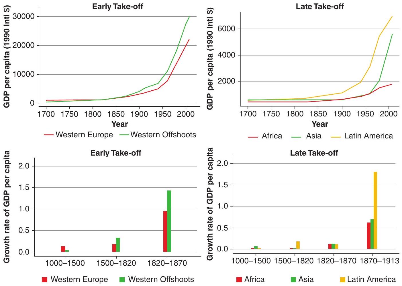
Then industrialisation happened.2 Gradually, first picking up steam (figuratively, but also literally!) in England in the mid- to late-18th century, and spreading over Western Europe and the U.S. through the 19th century, the growth rate of output per capita started a sustained increase by an order of magnitude. Eventually, this reached most other places in the world somewhere along the 20th century. Still, this initial takeoff was marked by the Great Divergence - a testament to the power of growth rates in changing living standards over time. The first countries to industrialise started to grow richer and richer, leaving behind the laggards (Figure 10.2). It also brought along a marked increase in urbanisation, with people flocking from rural areas to the more dynamic urban centers, which could now sustain substantially larger (and increasing) populations.
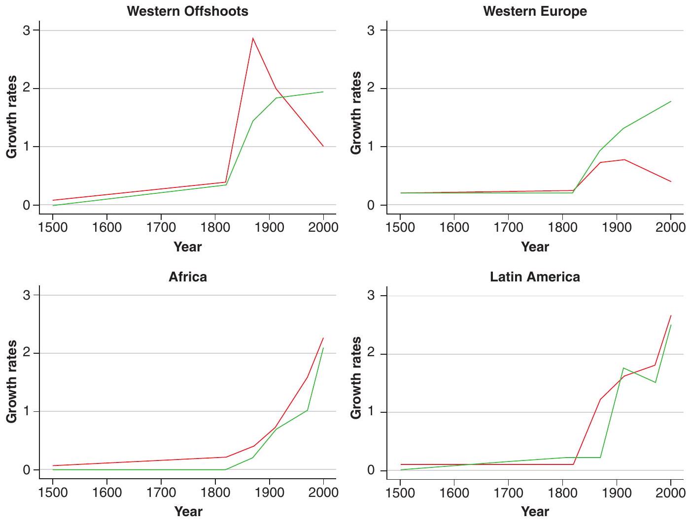
Still, this is not what we would call the full-on, modern, sustained growth regime. Why? Because a remnant of the Malthusian past remained. There remained a positive link between increased productivity and income per capita, on one side, and increased population on the other, as can be seen readily, for different parts of the world, in Figure 10.3. As such, part of the sustained increase in productivity growth was still being dissipated over more capitas.
However, a very important transition was taking place at the same time: the rise of human capital. The acceleration in productivity growth and income per capita was accompanied by rising literacy rates, schooling achievement, and improving health. This increase in human capital seems to be driven by the fact that the industrialisation process, particularly in its later stages, requires more and more “brain” relative to “brawn” - an educated, decently healthy workforce becomes a sine qua non.
10.1.2 Sustained economic growth
Then the demographic transition happened. At some point, human societies escaped definitively from the Malthusian shackles. Population growth ceased to be positively related to income per capita, and the relationship was actually reversed, with sharp declines in fertility rates. Even from a basic arithmetic perspective, this opens up the way for a historically astonishing rate of increase in living standards. In fact, the regions that first went into this transition reach a sustained speed of about 2% annual growth in income per capita over the last century or so - a rate at which living standards double in the space of one generation (35 years). Simultaneously, the relative importance of human capital increased even further, which was met by the first efforts in mass public education.
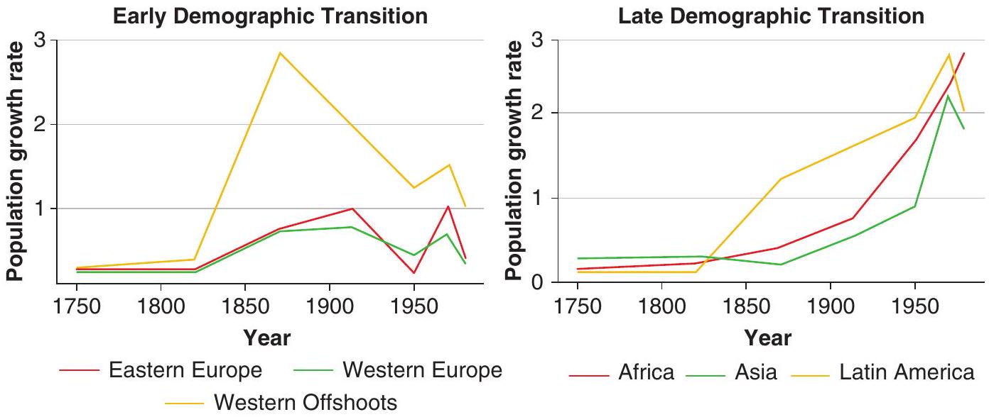
The demographic transition, i.e. the decline in fertility rates (accompanied by lower mortality and higher life expectancy), happened first in the leading industrialised nations, but then eventually reached the latecomers, as illustrated in Figure 10.4. (The exception for the moment, as we can see, is still Africa.) It actually had a three-fold impact on the growth process. First, and most obviously, it ceased the dilution of capital (and land). Second, it actually enabled the increased investment in human capital. Put simply, the tradeoff between quantity of children and the quality of the investment made in each one of them turned decisively towards the latter. Third, and more temporarily, it yielded a demographic dividend: a relatively large labour force, with relatively few young dependents.
10.2 A “unified” theory
Unified growth theory attempts to provide a single framework that can explain why growth may accelerate. One such mechanism relates to family decisions, i.e. whether to raise more kids or to raise fewer but more educated kids. Growth will force parents to educate their children at the expense of quantity of children, setting off an accelerating pattern.
The challenge is thus to come up with a framework that encompasses all the stylised facts spelled out in the previous section. In other words, we need a theory that has room for the Malthusian era, but then explains (i.e. endogenously generates) the transition to a post-Malthusian equilibrium with sustained productivity growth brought about by industrialisation and the attending increased importance of human capital. It must also account for the demographic transition and the possibility of sustained increases in living standards.
One could have told a story in which we combine the neoclassical growth model (which, after all, has zero growth in living standards in the long run) with the eventual takeoff of productivity being accounted for by the world of the endogenous growth models. However, how do we explain when and why we would move from one world to the other? And how do we incorporate the demographic aspect that seems to be such a central part of the story, and which lies thoroughly outside of the theories that we have seen so far?
We will start by sketching a model of parental investment that explains the links between demographic trends and productivity, while keeping the evolution of productivity exogenous. We will then endogenise productivity growth in order to complete our full very-long-run picture.
10.2.1 A simple model of the demographic transition
Consider a discrete-time framework in which individuals live for two periods, as in our basic OLG model, but now each individual, instead of coming into the economy out of nowhere, has a single parent. In the first period of life (childhood), individuals consume a fraction of their parent’s endowment of time (normalised to 1). This fraction will have to be greater to increase the child’s quality. In the second period of life (parenthood), individuals are endowed with one unit of time, which they allocate between child-rearing and labour force participation. At this stage, the individual’s problem is to choose the optimal mixture of quantity and quality of (surviving) children and supply their remaining time in the labour market, consuming their wages.
Let us consider the building blocks of this model in order.
Production
We assume that output is produced using land (exogenous and constant over time) and (efficiency units of) labour. We capture this using a constant returns to scale (CRS) production function:
\[ Y_{t}=H_{t}^{\alpha}\left(A_{t} X\right)^{1-\alpha}, \tag{10.1}\]
where \(Y_{t}\) is total output, \(H_{t}\) is total efficiency units of labour, \(A_{t}\) is (endogenous) productivity, and \(X\) is land employed in production. We can write this in per worker terms as
\[ y_{t}=h_{t}^{\alpha} x_{t}^{1-\alpha}, \tag{10.2}\]
where \(y_{t}=\equiv \frac{Y_{t}}{L_{t}}, h_{t}=\equiv \frac{H_{t}}{L_{t}}\), and \(x_{t}=\equiv \frac{A_{t} X}{L_{t}}\) (we can think of \(x_{t}\) as effective (land) resources per worker).
Preferences
An individual who is a parent in time \(t\) cares about consumption \(c_{t}\), and also about the number of children \(n_{t}\), and their quality \(h_{t+1}\). We summarise this in the following utility function:
\[ u^{t}=c_{t}^{1-\gamma}\left(n_{t} h_{t+1}\right)^{\gamma} . \tag{10.3}\]
We assume that individuals need to consume at least a subsistence level \(\tilde{c}\), which will be very important for the results. Children are passive recipients of their parents’ decisions. This means that this is not a full-fledged OLG model, such as the ones we have seen before, in which young and old made meaningful economic decisions, which in turn entailed intergenerational conflicts of interest. The OLG structure here is more meant to highlight the demographic structure of the problem.
Budget constraint
Let \(\tau\) be the amount of time needed to raise a child, regardless of quality. Any additional quality that an individual parent in time \(t\) bestows upon each child (to be reflected in the quality \(h_{t+1}\) ) requires some additional effort, \(e_{t+1}\) (education). Whatever is left of the unit time endowment will be supplied in the labour market, in exchange for a wage of \(w_{t}\) (per efficiency unit of labour). We assume that there are no property rights over land, so that the individual rate of return on that is zero.
For an individual who was given quality \(h_{t}\) by her parent, we thus have
\[ c_{t} \leq w_{t} h_{t}\left(1-n_{t} \tau-n_{t} e_{t+1}\right) . \tag{10.4}\]
This simply states that the individual can consume up to the level of income that she obtains from paid work.
Note that we can rearrange this budget constraint as follows:
\[ c_{t}+w_{t} h_{t} n_{t}\left(\tau+e_{t+1}\right) \leq w_{t} h_{t} . \tag{10.5}\]
The RHS of this inequality, which we may call \(z_{t} \equiv w_{t} h_{t}\), corresponds to total potential income, i.e. the income that the individual would obtain if all of her time were devoted to paid work. We can then reinterpret the budget constraint as stating that the individual can choose to devote her potential income to consumption or to raising her children, and the cost of raising children is the foregone income.
10.2.2 Investing in human capital
We take human capital to be determined by a combination of individual quality and the technological environment. Specifically, we posit a function
\[ h_{t+1}=h\left(e_{t+1}, g_{t+1}\right), \tag{10.6}\]
where \(g_{t+1} \equiv \frac{A_{t+1}-A_{t}}{A_{t}}\) is the rate of technological progress. The idea is that \(\frac{\partial h}{\partial e}>0\) (more education leads to more human capital), and \(\frac{\partial h}{\partial g}<0\) (faster technological progress erodes previously acquired human capital by making it obsolete). We also assume that more education increases adaptability to technological progress, so that \(\frac{\partial^{2} h}{\partial g \partial e}>0\). In the absence of investment in quality, each individual has a basic-level human capital that is normalised to 1 in a stationary technological environment: \(h(0,0)=1\).
Solution
We can substitute (10.4) and (10.6) into (10.3) to obtain:
\[ u^{t}=\left(w_{t}\left[1-n_{t}\left(\tau+e_{t+1}\right)\right] h_{t}\right)^{1-\gamma}\left(n_{t} h\left(e_{t+1}, g_{t+1}\right)\right)^{\gamma} . \tag{10.7}\]
Parents will choose \(n_{t}\) and \(e_{t+1}\) (how many children to have, and how much to invest in the education of each one of them) in order to maximise this utility. The FOC with respect to \(n_{t}\) will yield:
\[ (1-\gamma) c_{t}^{-\gamma}\left(n_{t} h\left(e_{t+1}, g_{t+1}\right)\right)^{\gamma} w_{t} h_{t}\left(\tau+e_{t+1}\right)=\gamma c_{t}^{1-\gamma} n_{t}^{\gamma-1} h\left(e_{t+1}, g_{t+1}\right)^{\gamma} \Rightarrow \tag{10.8}\]
\[ \frac{c_{t}}{w_{t} h_{t}}=\frac{1-\gamma}{\gamma} n_{t}\left(\tau+e_{t+1}\right) . \tag{10.9}\]
Note, from (10.4), that the LHS of this equation is the fraction of time devoted to labour market activities, \(1-n_{t}\left(\tau+e_{t+1}\right)\). It follows immediately that the individual will choose to devote a fraction \(\gamma\) of her time to child-rearing, and a fraction \(1-\gamma\) to labour.
The FOC characterises an interior solution, however, and we must take into account the subsistence consumption constraint. If \((1-\gamma) w_{t} h_{t}<\tilde{c}\), it follows that the interior solution would not be enough to sustain the individual. In that case, the subsistence constraint is binding, and the optimal thing to do is to work as much as needed to reach \(\tilde{c}\), and devote whatever is left to child-rearing. In other words, any individual whose potential income is below \(\tilde{z} \equiv \frac{\tilde{c}}{1-\gamma}\) will be constrained to subsistence consumption, and to limited investment in their kids.
This means that, below subsistence level, increases in potential income generate no increase in consumption, and an increase in the time spent raising kids (number and quality). After the subsistence threshold, it is consumption that increases, while the time spent in child-rearing stays flat.
How about the choice of education, \(e_{t+1}\) ? With some algebra, you can show that the FOC with respect to \(e_{t+1}\) can be written as
\[ \frac{\gamma}{1-\gamma} \frac{c_{t}}{n_{t} w_{t} h_{t}}=\frac{h\left(e_{t+1}, g_{t+1}\right)}{\frac{\partial h}{\partial e}} . \tag{10.10}\]
Substituting the LHS using (10.9), we get the following:
\[ \tau+e_{t+1}=\frac{h\left(e_{t+1}, g_{t+1}\right)}{\frac{\partial h}{\partial e}}, \tag{10.11}\]
which implicitly defines \(e_{t+1}\) as a function of the productivity growth rate \(g_{t+1}\). Using the implicit function theorem, we can see that, as long as \(h\) is decreasing in \(g\), and concave in \(e\), as we have assumed, \(e_{t+1}\) will be increasing in \(g_{t+1}\). In other words, parents will choose to invest in more education when productivity grows faster, because education increases adaptability and compensates for the erosion of human capital imposed by technological change.
But how about the number of children? It is easy to see that there is no link between wages and the choice between quantity \(\left(n_{t}\right)\) and quality \(\left(e_{t+1}\right)\) in child-rearing: potential income doesn’t show up in (10.11), and (10.9) only speaks to the overall amount of time (i.e. number times quality). However, (10.11) shows that productivity growth does affect that tradeoff: \(n_{t}\) doesn’t show up in that equation, but \(e_{t+1}\) does. This means that an increase in \(g\) will increase the quality of kids, and reduce their quantity to keep consistency with (10.9).
In sum
This simple model therefore predicts a number of key stylised facts regarding the demographic transition:
An increase in (potential) income raises the number of children, but has no effect on their quality, as long as the subsistence constraint is binding.
An increase in (potential) income does not affect the number of children and their quality, as long as the subsistence constraint ceases to be binding.
An increase in the rate of technological progress reduces the number of children and increases their quality.
The first two results are driven by the subsistence requirement. As long as it is binding, any increase in potential income will imply that fewer hours of work are needed to obtain subsistence and more time can be devoted to having children. However, if the rate of technological change is constant, this will be translated into a greater number of kids, and not in higher quality: the point about investing in quality is to counteract the erosion of human capital imposed by faster technological change. When the subsistence constraint is no longer binding, then increased potential income will be reverted into increasing consumption.
10.2.3 The dynamics of technology, education and population
In order to close the picture, we need to have a model of how technological progress takes place. Inspired by the models of endogenous growth that we have seen, we think of productivity growth being driven by the accumulation of knowledge, which is enhanced by human capital and by scale effects. Quite simply, we posit
\[ g_{t+1} \equiv \frac{A_{t+1}-A_{t}}{A_{t}}=g\left(e_{t}, L_{t}\right), \tag{10.12}\]
where \(g(\cdot, \cdot)\) is increasing and concave in both arguments: more and more educated people increase the rate of growth, at decreasing rates. (Remember that our discussion of scale effects argued that there is good evidence for their presence in this very long-run context, as per the models of innovation studied in Chapter 6 and synthesised in Kremer (1993).)
Obviously, the evolution of the size of the adult population is described by \(L_{t+1}=n_{t} L_{t}\), since \(n_{t}\) is the number of children that each individual adult alive at time \(t\) chooses to have. The model of demographic decisions shows that \(n_{t}\) is a function of the rate of technological progress and, when the subsistence constraint is binding, also of potential income. Potential income, in turn, is a function of the existing technology, education levels, and the amount of effective resources per worker.
The one thing that is missing is the evolution of potential resources per worker, \(x_{t} \equiv \frac{A_{t} X}{L_{t}}\), but that is easy to state: \(x_{t+1}=\frac{1+g_{t+1}}{n_{t}} x_{t}\), that is, effective resources per worker grow at the rate of productivity, adjusted by the growth of population.
We now have a dynamic system in four variables: \(g_{t}, x_{t}, e_{t}\), and \(L_{t}\). These capture all of our variables of interest, namely productivity growth, productivity levels, human capital investment, and population.
Closing the model
The dynamics of the model can be analysed graphically, and we start by looking at the joint evolution of education and technology. Since the dynamics of education and technological progress are not affected by whether the subsistence constraint is binding, we can analyse then independently, as depicted in Figure 10.5. If population is small (Panel A), the rate of technological progress is slow because of scale effects. Then the only steady state is with zero levels of education: it is not worth investing in the quality of children, since the erosion caused by technological progress is really small. However, as population size grows, which the \(g\) curve shifts up, until we end up in the world of Panel B. Here there are two additional positive-education steady states ( \(e_{M}\) and \(e_{h}\), which is stable). As population grows even larger, we end up in Panel C, with a unique, stable steady state with high levels of educational investment.
10.3 The full picture
Figure 10.5 encompasses all of our story, from the Malthusian regime to sustained growth. Consider an economy in early stages of development. Population size is relatively small and the implied slow rate of technological progress does not provide an incentive to invest in the education of children: this is the world of Figure 10.5A - the Malthusian Regime. Over time, the slow growth in population that takes place in the Malthusian Regime raises the rate of technological progress and shifts the \(g\) in
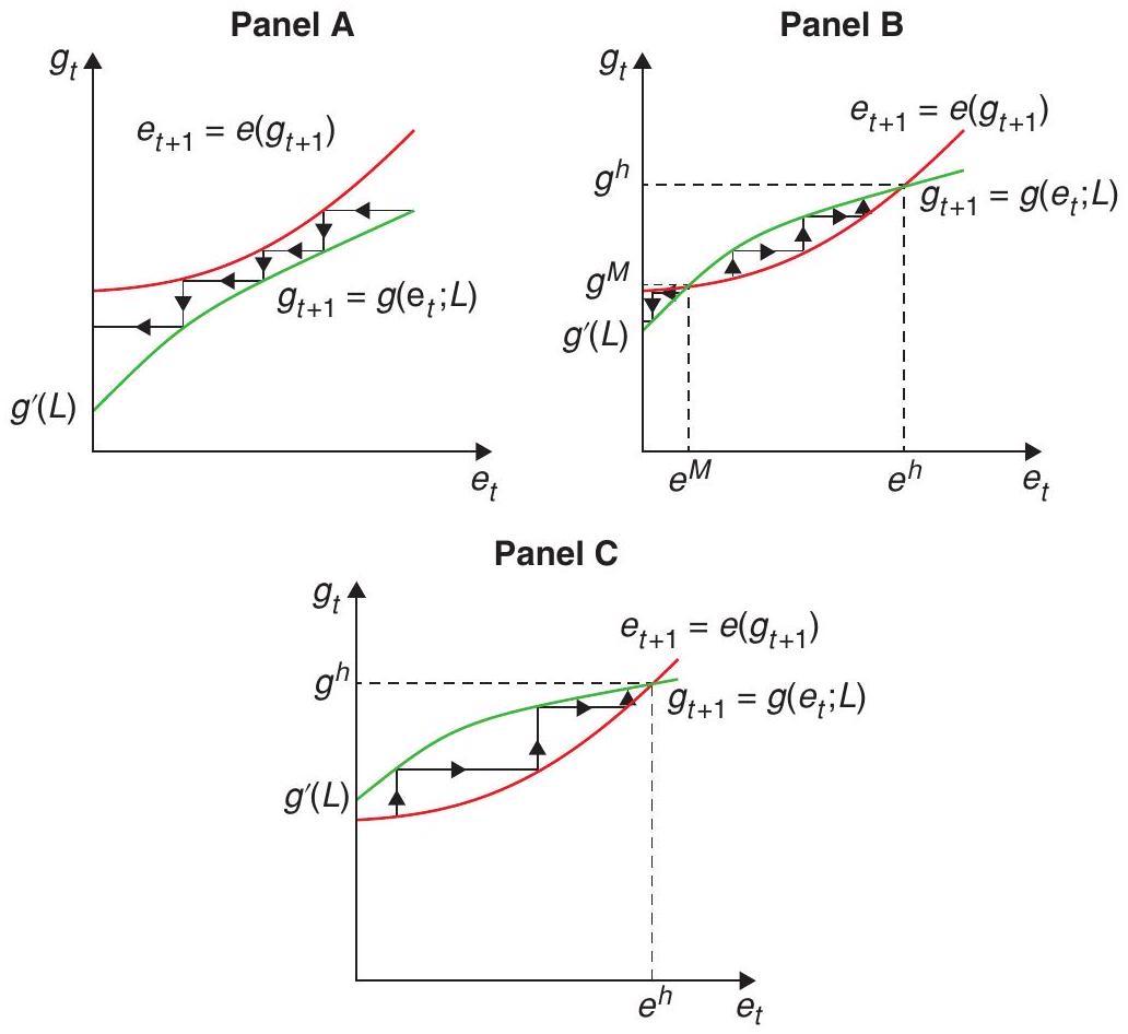
Panel A enough to generate a qualitative change to Panel B. This is characterised by multiple, history-dependent, stable steady-state equilibria: some countries may take off and start investing in human capital, while others lag behind. However, since the economy started in the Malthusian steady state, it initially sticks in the vicinity of that steady state, which is still stable in the absence of major shocks.
Eventually, the continued increase in population leads us to Panel C: the Malthusian steady state disappears, and the economy starts converging to the steady state with high education. The resulting increase in the pace of technological progress, due to the increased levels of education, has two opposing effects on the evolution of population. On the one hand, it allows for the allocation of more resources for raising children. On the other hand, it induces a reallocation of these additional resources toward child quality. Initially, there is low demand for human capital, and the first effect dominates: this is the Post-Malthusian Regime.
The interaction between investment in human capital and technological progress generates a virtuous circle: human capital formation pushes faster technological progress, which further raises the demand for human capital, which fosters more investment in child quality. Eventually, the subsistence constraint seizes to bind, triggering a demographic transition and sustained economic growth.
10.4 What have we learned?
In sum, this theory explains growth over the very long run by marrying the insights of endogenous growth theory (the role of scale effects and human capital in increasing the growth rate of productivity) to a theory of endogenous population growth and human capital investment. In the presence of a subsistence level of consumption, this marriage produces an initial period of stagnation, and the eventual transition to sustained economic growth with high levels of human capital investment and the demographic transition.
10.5 What next?
For those interested in this transition Galor (2005) is a great starting point.
References
Galor, O. (2005). From stagnation to growth: Unified growth theory. Handbook of Economic Growth, 1, 171-293.
Kremer, M. (1993). Population growth and technological change: One million B.C. to 1990. The Quarterly Journal of Economics, 108(3), 681-716.
Notice that the Kremer model does not solve this riddle. Even though it starts from a Malthusian framework, by assuming a specific process of economic growth, it only explains the divergent part of the story.↩︎
While industrialisation is considered the turning point for economic growth, arguably their impact was possible (or at least complemented) by two other world-changing events occurring at the same time. First, the French Revolution that dismantled the segmented labour market of the middle ages, opened up labour so that anybody could find his or her best use of their own abilities, thus increasing productivity dramatically. Second, the U.S. Constitution; a key attempt to have a government controlled by its citizens and not the other way around. Reigning in the authoritarian tendencies or the possibility of capricious use of resources also provided significant productivity gains through better infrastructure and better public goods provision.↩︎