20 Rules vs Discretion
Now, let’s move back to the New Keynesian world of Chapter 15 where the existence of nominal rigidities implies that monetary policy (MP) can have real effects. Most central banks believe this a more realistic description of the environment, at least in the short run. In such a world, MP has to assess the trade-offs when it comes to stabilising inflation versus stabilising output. In this chapter we develop a framework that will let us analyse this.
20.1 A basic framework
Fortunately, we have already developed most of the ingredients of such framework: it’s the canonical New Keynesian model! As you may recall, it is founded on two basic equations, the New Keynesian IS curve (NKIS), and the New Keynesian Phillips curve (NKPC), which we rewrite here for your convenience. First, the NKIS:
\[ y_{t}=E_{t}\left[y_{t+1}\right]-\sigma\left(i_{t}-E_{t}\left[\pi_{t+1}\right]-\rho\right)+u_{t}^{I S} . \tag{20.1}\]
This is exactly as we had before, with \(u_{t}^{I S}\) corresponding to an (aggregate demand) shock. We specify shocks being a random, white-noise disturbance.
Now, the NKPC:
\[ \pi_{t}=\kappa\left(y_{t}-y_{t}^{n}\right)+\beta E_{t}\left[\pi_{t+1}\right]+u_{t}^{\pi}, \tag{20.2}\]
with \(u_{t}^{\pi}\) corresponding to an (aggregate supply) shock. If you check this against the specification of previous chapters, the main difference you will notice is the existence of these demand and supply shocks.
You will recall that, when we discussed the canonical NK model, we talked about an interest rate rule, namely the celebrated Taylor rule. Now is the time to think about the nature of monetary policy rules more broadly.
20.1.1 Time inconsistency
The first thing we have to do is to think about what the central bank/policy-maker (CB, for shorthand) wants to do. We assume that, when it comes to inflation, it wants to minimise departures from the optimal level, which we normalize to zero. (Again, it could be positive, could be negative - it’s just
a normalization.) When it comes to output, we will introduce a more consequential assumption: we take that the CB wants to minimise deviations not from the natural rate \((y)\), but rather from what we may call the Walrasian rate of output, which we call \(y^{*}\). Think of this as the output level that would prevail in the absence of any market distortions, such as monopoly power or distortionary taxation. The idea is that it is almost surely the case that \(y^{*}>y\)-monopolies produce suboptimal quantities, distortionary taxes lead to suboptimal effort, etc.
In order to capture this idea, we will usually think of the CB as minimising a loss function like this:
\[ L=\frac{1}{2}\left[\alpha \pi_{t}^{2}+\left(y_{t}-y^{*}\right)^{2}\right], \tag{20.3}\]
where \(\alpha>0\) denotes the relative importance of inflation as compared to output deviations.
To discuss the implications, let’s develop a model to deal with this issue in the spirit of Rogoff (1985). The details follow Velasco (1996) which uses a simpler Phillips curve, but which captures the spirit of (20.2). In this simplified version the economy is fully characterised by the expectational Phillips curve
\[ y_{t}-y=\theta\left(\pi_{t}-\pi_{t}^{e}\right)+z_{t}, \quad \theta>0, \tag{20.4}\]
where \(\pi\) is the actual rate of inflation, \(\pi^{e}\) is the expected rate, \(y_{t}\) is actual output, \(y\) is steady state (or natural rate) output, and \(z_{t}\) is a random shock (which should be interpreted here as a supply shock) with mean zero and variance \(\sigma^{2}\). The term \(\theta\left(\pi_{t}-\pi_{t}^{e}\right)\) implies that whenever actual inflation is below expected inflation, output falls. Notice that the supply shock is the only shock here (we assume away demand shocks, whether of the nominal or real kind).
The social loss function is
\[ L=\left(\frac{1}{2}\right)\left(\alpha \pi_{t}^{2}+\left(y_{t}-\gamma y\right)^{2}\right), \quad \alpha>0, \gamma>1 . \tag{20.5}\]
The function (20.5) indicates that society dislikes fluctuations in both inflation and output. Notice that the bliss output rate is \(y^{*}=\gamma y\), is above the natural rate of \(y\). This will be a source of problems.
The timing of actions is as follows. The economy has a natural output rate \(y\) which is known by all players. The public moves first, setting its expectations of inflation. The shock \(z_{t}\) is then realised. The policymaker moves next, setting \(\pi\) to minimise (20.5) subject to (20.4), the realisation of the shock (known to the policymaker) and the public’s expectations of inflation. Notice this timing implies the policymaker has an informational advantage over the public.
By assuming that the policymaker can control \(\pi_{t}\) directly, we are finessing the issue of whether that control is exercised via a money rule (and, therefore, flexible exchange rates), an interest rate rule, or an exchange rate rule. What is key is that the authorities can set whatever policy tool is at their disposal once expectations have been set.
The policy maker, acting with discretion sets, \(\pi_{t}\) optimally, taking \(\pi_{t}^{e}\) (which has been already set) as given. Substituting (20.4) into (20.5) the objective function becomes
\[ L=\left(\frac{1}{2}\right) \alpha \pi_{t}^{2}+\left(\frac{1}{2}\right)\left[\theta\left(\pi_{t}-\pi_{t}^{e}\right)+z_{t}-y(\gamma-1)\right]^{2} . \tag{20.6}\]
Minimising with respect to \(\pi_{t}\) yields
\[ \alpha \pi_{t}+\theta\left[\theta\left(\pi_{t}-\pi_{t}^{e}\right)+z_{t}-y(\gamma-1)\right]=0 . \tag{20.7}\]
Rearranging we arrive at
\[ \theta \pi_{t}=(1-\lambda)\left[\theta \pi_{t}^{e}-z_{t}+y(\gamma-1)\right], \tag{20.8}\]
where \(\lambda \equiv \frac{\alpha}{\alpha+\theta^{2}}<1\).
If, in addition, we impose the rational expectations condition that \(\pi_{t}^{e}=E \pi_{t}\), we have from (20.8) that
\[ \theta \pi_{t}^{e}=\left(\frac{1-\lambda}{\lambda}\right)(\gamma-1) y . \tag{20.9}\]
Hence, under discretion, inflation expectations are positive as long as \((\gamma-1) y\) is positive. Since \((\gamma-1) y\) is the difference between the natural rate of output and the target rate in the policymaker’s loss function, we conclude that, as long as this difference is positive, the economy exhibits an inflation bias: expected inflation is positive.
\[ \theta \pi_{t}=\left(\frac{1-\lambda}{\lambda}\right)(\gamma-1) y-(1-\lambda) z_{t}, \tag{20.10}\]
or, more simply,
\[ \pi_{t}=\left(\frac{1-\lambda}{\theta \lambda}\right)(\gamma-1) y-\frac{(1-\lambda)}{\theta} z_{t}, \tag{20.11}\]
so that actual inflation depends on the shock as well as on the fixed inflation bias term. The fact that the CB wants to boost output above its natural level leads to a problem of dynamic inconsistency and inflationary bias that was originally pointed out by Kydland and Prescott (1977), and Barro and Gordon (1983). This is one of the most important and influential results for modern macroeconomic policy-making, and its intuition points squarely at the limits of systematic policy in a world where people are rational and forward-looking: they will figure out the CB’s incentives, and, because of that, the tradeoff that the CB would like to exploit vanishes. Rational expectations implies that the equilibrium will occur at an inflation rate sufficiently high so that the cost of increasing inflation further would not be desirable to the CB. Once this anticipation is included in the model, discretion does not help expand output. In fact, if all could agree to a lower inflation, everybody would be better off.
The main takeaway is that credibility is a key element of monetary policy practice: if people believe the CB’s commitment to fight inflation and not to exploit the inflation-output tradeoff systematically, the terms of the tradeoff in the short run become more favourable. This idea has been encapsulated in the mantra of rules vs discretion: policy-makers are better off in the long run if they are able to commit to rules, rather than trying to make policy in discretionary fashion.
20.1.2 A brief history of monetary policy
In common policy parlance, the lesson is that being subject to time inconsistency, the CB needs to find an anchor for monetary policy. This anchor helps keep inflation expectations in check, and ameliorate the time inconsistency problem. The drawback is that the anchor may be too rigid, and make monetary policy less effective or have other side effects. Therefore the key issue is how to find an anchor that delivers credibility while not jeopardising the ability to react to shocks. One such mechanism is to appoint conservative central bankers,1 who would have a low \(\gamma\); or insuring the independence of the CB and having it focus squarely on inflation. These two policies, now widely used, have helped to reduce the inflation bias as shown in Figure 20.1. But in addition to these obvious solutions, the quest to build a monetary framework that provides credibility and flexibility has gone on for decades. Mishkin (1999)) provides a nice narrative that we summarize as follows:
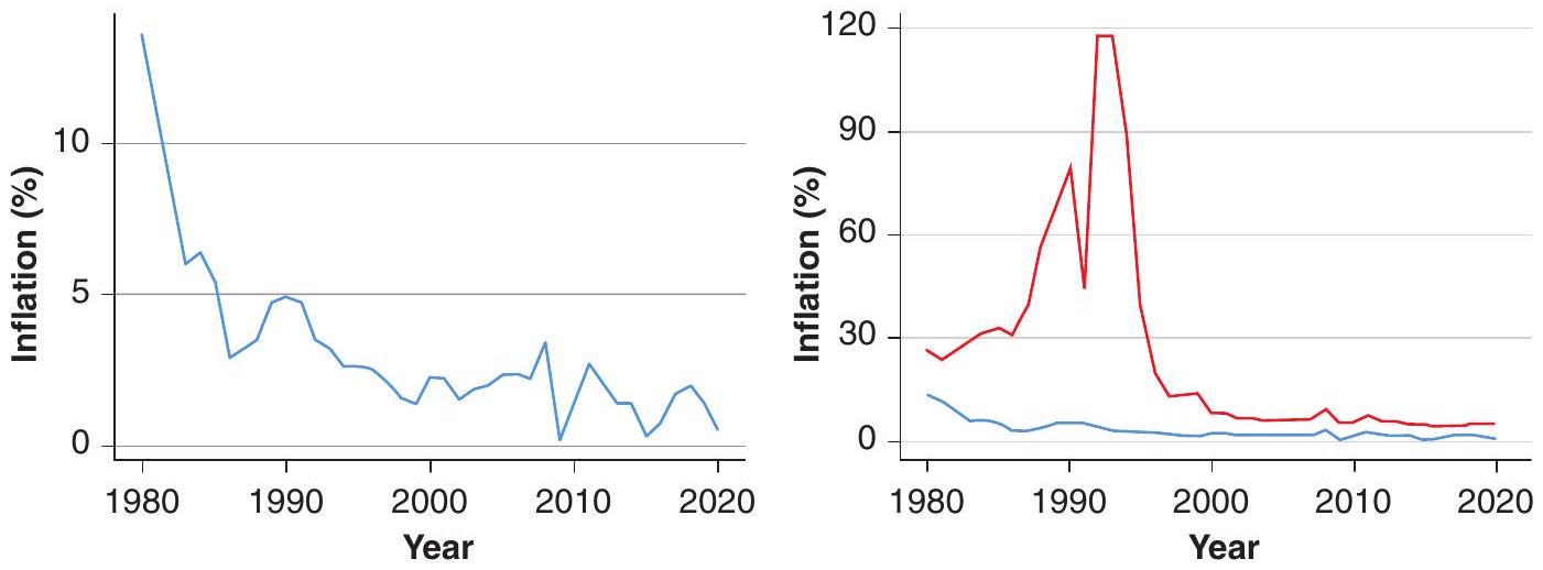
The age of discretion lasted until the early 70s when there was a belief that there was a long term tradeoff between inflation and output. During this period there were no major objections to the use of monetary policy. The Keynesian/monetarist debate focused on the relative merits of fiscal vs. monetary policy.
The rise of inflation in the 1970s led to increased skepticism on the role of monetary policy, and led to the acknowledgement that a nominal anchor was required. The discussion took place mostly in the U.S., as most other countries still had a fixed exchange rate that they carried over from the Bretton Woods system (and therefore no monetary policy of their own). But once countries started recovering their monetary policies by floating the exchange rate, monetary aggregates became the prime nominal anchor. Central banks committed to a certain growth in monetary aggregates over the medium term, while retaining flexibility in the short run.
By the 1980s, it was clear that monetary aggregate targeting was not working very well, mostly due to instability in the demand for money. Gerald Bouey, then governor of the Bank of Canada, described the situation in his famous quote “We didn’t abandon monetary aggregates, they abandoned us.”
Starting in the 1990s, central banks have increasingly used inflation itself as the nominal target. This is the so called inflation targeting regime. Other central banks (the Fed in the U.S.) have remained committed to low inflation, but without adopting an explicit target (though Fed governors embrace openly the idea of a 2% target for annual inflation recently updated to “an average of 2% over time”). Other countries remained using fixed exchange rates, while monetary targeting went in disuse.
Inflation targeting, however, has a drawback: it magnifies output volatility when the economy is subject to substantial supply shocks. As a response many central bankers do not run a strict inflation targeting but a flexible inflation targeting, where the target is a long run objective retaining substantial flexibility in the short run.2
More recently, some central banks have veered away from targeting inflation and started targeting inflation expectations instead (see Adrian et al. (2018)).
20.2 The emergence of inflation targeting
Given its increasing popularity, let’s spend some time analysing the monetary framework of inflation targeting. We laid the framework above which gave us a solution for the inflation rate.
Recall that using (20.9) in (20.8) yields
\[ \theta \pi_{t}=\left(\frac{1-\lambda}{\lambda}\right)(\gamma-1) y-(1-\lambda) z_{t}, \tag{20.12}\]
so that actual inflation depends on the shock as well as on the fixed inflation bias term. Subtracting (20.9) from (20.12) yields
\[ \theta\left(\pi_{t}-\pi_{t}^{e}\right)=-(1-\lambda) z_{t}, \tag{20.13}\]
or
\[ y_{t}=y+\lambda z_{t} . \tag{20.14}\]
That is, deviations of output from the natural rate are random and depend on the shock and on the parameter \(\lambda\).
Finally, using (20.12) and (20.14) in (20.5) yields
\[ L=\left(\frac{1}{2}\right)\left(\frac{1-\lambda}{\lambda}\right)\left[(\gamma-1) y-\lambda z_{t}\right]^{2}+\left(\frac{1}{2}\right)\left(y(1-\gamma)+\lambda z_{t}\right)^{2}, \tag{20.15}\]
and taking expectations we have
\[ L=\left(\frac{1}{2}\right)\left(\frac{1}{\lambda}\right)\left[(\gamma-1)^{2} y^{2}+\lambda^{2} E z_{t}^{2}\right], \tag{20.16}\]
or
\[ E L^{d i s c}=\left(\frac{1}{2}\right)\left[\frac{(\gamma-1)^{2} y^{2}}{\lambda}+\lambda \sigma^{2}\right], \tag{20.17}\]
where \(\sigma^{2}\) is the variance of \(z_{t}\) and the expectation is unconditional - that is, taken without knowing the realisation of \(z_{t}\). Hence, expected social loss is increasing in the natural rate \(y\), in the difference between \(\gamma\) and 1, and in the variance of the shock.
20.2.1 A rigid inflation rule
Consider what happens, on the other hand, if the policymaker has precommitted not to manipulate inflation, therefore setting \(\pi_{t}=0\). The Phillips curve dictates that
\[ y_{t}=y-\theta \pi_{t}^{e}+z_{t} . \tag{20.18}\]
If, in addition, the rule is credible, so that \(\pi_{t}^{e}=0\), we have
\[ y_{t}=y+z_{t} . \tag{20.19}\]
Notice that, unlike the case of discretionary policy (see expression (20.14)), here output absorbs the full impact of the shock (the coefficient \(\lambda\) is missing).
The corresponding loss is
\[ L^{\text {rule }}=\left(\frac{1}{2}\right)\left[-y(\gamma-1)+z_{t}\right]^{2} . \tag{20.20}\]
The unconditional expectation of (20.20) is
\[ E L^{r u l e}=\left(\frac{1}{2}\right)\left[y^{2}(\gamma-1)^{2}+\sigma^{2}\right] . \tag{20.21}\]
20.2.2 | Which regime is better?
If the unconditional expectation of the loss is the welfare criterion, then deciding which regime is better depends on parameter values. Expressions (20.17) and (20.21) reveal that \(E L^{\text {rule }}<E L^{\text {disc }}\) if and only if \((\gamma-1) y>\sigma \sqrt{\lambda}\). The LHS is a proxy for the inflation bias under discretion; the RHS is a proxy for the variability cost under a rigid rule. The rigid rule is better when the former is larger, and vice versa. In short, you prefer a fixed rule if your inflation bias is large and the supply shocks small.
20.2.3 | The argument for inflation targeting
Suppose now that the social objective function is still given by (20.5), but that now the policymaker is given the objective function
\[ L^{p}=\left(\frac{1}{2}\right) \alpha\left(\pi_{t}+\pi\right)^{2}+\left(\frac{1}{2}\right)\left(y_{t}-\gamma y\right)^{2}, \tag{20.22}\]
where \(-\pi\) is the bliss rate of inflation for the policymaker. We can interpret this as the target assigned to the policymaker by society.
Substituting (20.4) into (20.22), one gets
\[ L^{p}=\left(\frac{1}{2}\right) \alpha\left(\pi_{t}+\pi\right)^{2}+\left(\frac{1}{2}\right)\left[\theta\left(\pi_{t}-\pi_{t}^{e}\right)+z_{t}-(\gamma-1) y\right]^{2} . \tag{20.23}\]
Minimising with respect to \(\pi_{t}\) yields
\[ \alpha\left(\pi_{t}+\pi\right)+\theta\left[\theta\left(\pi_{t}-\pi_{t}^{e}\right)+z_{t}-(\gamma-1) y\right]=0 . \tag{20.24}\]
Rearranging we arrive at
\[ \theta \pi_{t}=(1-\lambda)\left[\theta \pi_{t}^{e}-z_{t}+y(\gamma-1)\right]-\lambda \theta \pi . \tag{20.25}\]
Taking expectations we have
\[ \theta \pi_{t}^{e}=\left(\frac{1-\lambda}{\lambda}\right)(\gamma-1) y-\theta \pi, \tag{20.26}\]
so the inflation bias is positive or negative depending on the setting of \(\pi\). Suppose the target is set so that the inflation bias is zero. Having \(\theta \pi_{t}^{e}=0\) implies
\[ \lambda \theta \pi=(1-\lambda)(\gamma-1) y . \tag{20.27}\]
Using this in (20.25) yields
\[ \theta \pi_{t}=-(1-\lambda) z_{t} . \tag{20.28}\]
Using this and \(\pi_{t}^{e}=0\) in (20.4) yields
\[ y_{t}-y=\lambda z_{t}, \tag{20.29}\]
so that deviations of output from its long run level are the same as under discretion.
Finally, using (20.28) and (20.29) into the public’s loss function (20.5) yields
\[ L=\left(\frac{1}{2}\right) \lambda(1-\lambda) z_{t}^{2}+\left(\frac{1}{2}\right)\left[\lambda z_{t}-(\gamma-1) y\right]^{2} . \tag{20.30}\]
Taking expectations and rearranging
\[ E L^{\text {target }}=\left(\frac{1}{2}\right)\left[\lambda \sigma^{2}+(\gamma-1)^{2} y^{2}\right] . \tag{20.31}\]
It is easy to check that \(E L^{\text {target }}\) is smaller than either \(E L^{\text {disc }}\) or \(E L^{\text {rule }}\). That is, inflation targeting is better for welfare than fully discretionary policy and a rigid rule. The intuition should be simple: targeting enjoys the flexibility benefits of discretion and the credibility benefits of a rule (the inflation bias is zero).
20.2.2 In sum
As inflation in the world decreased, monetary policy entered into a happy consensus by the 2000s. Credibility had been restored, and even those central banks that did not explicitly target inflation were widely understood to be essentially doing the same. The short-term interest rate was the policy tool of choice. Enhanced credibility, or the so called “flattening of the Phillips curve” made monetary policy more powerful as a stabilisation mechanism, and as a result became the tool of choice for steering the business cycle. Some central bankers even acquired heroic, pop-culture status.
But then, the 2008/2009 crisis hit. The consensus was revealed inadequate to deal with the crisis at its worst, and questions were raised as to the extent to which monetary policy had failed to prevent (and perhaps contributed to) the Great Recession and, later on, the European Crisis. Perhaps with the benefit of hindsight, the challenge proved to be central bank’s finest hour: the recoveries were relatively swift and inflation remained low. The hard-gained credibility provided the room for massive increases in liquidity, that shattered not a bit the credibility of the central banks and allowed to counteract the drainage of liquidity during the crises. This was perhaps best epitomised in a celebrated quote by Mario Draghi, then governor of the European Central Bank who, in July 2012, announced that the Central Bank would do “whatever it takes”. This phrase, as of today, is the symbol of the coming of age of modern CB when full discretion can be pursued without rising an eyebrow or affecting expectations!
References
Adrian, T., Laxton, M. D., & Obstfeld, M. M. (2018). Advancing the frontiers of monetary policy. International Monetary Fund.
Barro, R. J. & Gordon, D. B. (1983). Rules, discretion and reputation in a model of monetary policy. Journal of Monetary Economics, 12(1), 101-121.
Kydland, F. E. & Prescott, E. C. (1977). Rules rather than discretion: The inconsistency of optimal plans. Journal of Political Economy, 85(3), 473-491.
Mishkin, F. S. (1999). International experiences with different monetary policy regimes. Journal of Monetary Economics, 43(3), 579-605.
Rogoff, K. (1985). The optimal degree of commitment to an intermediate monetary target. The Quarterly Journal of Economics, 100(4), 1169-1189.
Velasco, A. (1996). Fixed exchange rates: Credibility, flexibility and multiplicity. European Economic Review, 40, 1023-1035.
One way of illustrating this debate is to remember the discussion surrounding the creation of the European Central Bank. As a novel institution whose governance was in the hands of a number of countries, it was not clear how it would build its credibility. Someone suggested to locate it in Frankfurt, so it could absorb (by proximity?) Germany’s conservative approach to monetary policy. The french wanted to control the presidency, but this was considered not sufficiently strong at least at the beginning, so they compromised on a two year presidency with a Dutch. However, after two years, when French Jean Marie Trichet took over, he still had to be overly conservative to build his, and the institution’s, credibility.↩︎
We should also keep in mind that inflation targeting does not mean that the central bank or policy maker does not care about anything other than inflation. As we show in the model in the next section, the central bank’s objective function may take deviations of output into account - the relative weight of output will affect the tolerance of the central bank to deviations of inflation from the target as a result of shocks.↩︎