6  Endogenous growth models II: Technological change

As we’ve seen, the challenge of the endogenous growth literature is how to generate growth within the model, and not simply as an assumption as in the Neoclassical Growth Model (NGM) with exogenous technological progress. The basic problem with the NGM (without exogenous technological progress) was that the incentives to capital accumulation decreased with the marginal product of capital. So, if we are to have perpetual growth we need a model that somehow gets around this issue. To do so, the literature has gone two ways. One is to change features of the production function or introduce additional factors that are complementary to the factors that are being accumulated in a way that keep the incentives to accumulation strong. The other alternative is to endogenise technological change. The first approach was the subject of the previous chapter, this chapter will focus on the second one.

Our final discussion in the previous chapter already hinted at the issues that arise when endogenising technological change. Most crucially, knowledge or ideas have many of the properties of a public good. In particular, ideas might be (or be made) excludable (e.g. using patents or secrecy), but they are distinctly non-rival. Because of that, there is a big incentive to free-ride on other people’s ideas - which is a major reason why governments intervene very strongly in the support of scientific activities. We have already looked at stories based on externalities (from learning-by-doing) and specialisation. We have also seen how they give rise to a wedge between the decentralised equilibrium and the optimal rate of growth.

In this chapter, we will take this discussion further by properly studying models where technological change emerges endogenously, through firms purposefully pursuing innovation. This is not only for the pure pleasure of solving models - though that can also be true, if you are so inclined! In fact, we will be able to see how the incentives to innovate interplay with market structure. This in turn opens a window into how the links between policy domains such as market competition, intellectual property rights, or openness to trade are fundamentally related to economic growth. We will also see that it may be the case (perhaps surprisingly) that technological innovation - and, hence economic growth - may be too fast from a social welfare perspective.

There are two ways of modelling innovation: one where innovation creates additional varieties, and another where new products sweep away previous versions in a so-called quality ladder. In the product variety model, innovation introduces a new variety but it does not (fully) displace older alternatives, like introducing a new car model or a new type of breakfast cereal. This is very much along the lines of

the model of specialisation that we have already seen (and to which we will return later in the chapter). In the quality ladder approach (also known as the Schumpeterian model), a new variety is simply better than old versions of the same thing and displaces it fully. (Schumpeter famously talked about firms engaging in “creative destruction” - this is what gives this approach its name.) Examples we face everyday: typewriters wiped out by word-processing computer software; the USB keys phasing out the older 5.4-inch diskette, and in turn later being displaced by cloud storage; VCRs displaced by DVD players, and eventually by online streaming; lots of different gadgets being killed by smartphones, and so on. We will develop two standard models of innovation, one for each version, and discuss some of the most important among their many implications for policy.

6.1 Modelling innovation as product specialisation

Following up on the previous chapter, we develop a full-fledged model of innovation through the development of new product varieties. It highlights a few important points: the role of monopoly profits in spurring the pursuit of innovation by firms, and the presence of scale effects (larger economies grow faster).

We start with this version because it will be familiar from the previous chapter. It is the model of innovation through specialisation, from Romer (1990). While we then left unspecified the process through which innovation takes place - where did the new varieties come from, after all? - we will now take a direct look at that.

Let’s consider a slightly different version of the production function we posited then

\[ Y(X)=\left[\int_{0}^{M} X(i)^{\alpha} d i\right]^{\frac{1}{\alpha}} \tag{6.1}\]

where again \(X(i)\) stands for the amount of intermediate input of variety \(i\), and \(M\) is the range of varieties that are currently available. Recall that we treat each sector \(i\) as infinitesimally small within a continuum of sectors. We are leaving aside the role of labour in producing final output for simplicity. Instead, we will assume that labour is used in the production of intermediate inputs on a one-for-one basis so that \(X(i)\) also stands for the amount of labour used to produce that amount of intermediate input.¹

How are new varieties developed? First of all, we must devote resources to producing new varieties - think about this as the resources used in the R&D sector. To be more concrete, let’s say we need workers in the R&D sector, which we will denote as \(Z_{M}\), and workers to produce intermediate inputs, which we will label \(Z\) to follow the notation from the previous chapter, where we had (somewhat vaguely) used that designation for the total resources devoted to intermediate inputs. It follows from this that \(Z \equiv \int_{0}^{M} X(i) d i\). To pin down the equilibrium, we will posit a labour market-clearing condition: \(Z_{M}+Z=L\), the total labour force in the economy, which we will assume constant. We will also take \(Z_{M}\) (and, hence, Z) to be constant.² We will assume that the production of new varieties is linear in R&D labour, and proportional to the existing stock of varieties, according to

\[ \dot{M}_{t}=B Z_{M} M_{t} . \tag{6.2}\]

Note also that we can use in (6.1) the fact that each symmetric intermediate sector in equilibrium will use \(X(i)=\bar{X}=\frac{Z}{M}\), given the definition of Z, just as in the previous chapter. This means we can write

\(Y_{t}=M^{\frac{1-\alpha}{\alpha}} Z\). Given that \(Z\) is constant, it follows that \(Y\) grows at \(\frac{1-\alpha}{\alpha}\) times the growth rate of \(M\), and, hence (using (6.2)) the growth rate of \(Y\) is \(\frac{1-\alpha}{\alpha} B Z_{M}\). It follows that, to figure out the growth rate of the economy, we need to figure out the amount of resources devoted to producing new varieties, \(Z_{M}\). In short, just as in the previous chapter, economic growth comes from the amount of resources devoted to the R&D sector, which is what drives innovation.

So we need to figure out what determines \(Z_{M}\). For that, we need to start by positing the market structure in this economy, in terms of the intermediate inputs, final output, and the production of varieties. On the first, we assume that each variety is produced by a monopolist that holds exclusive rights to it. The final output is then produced by competitive firms that take the price of inputs as given as well. What would one of these competitive firms do? They would try to minimise the cost of producing each unit of output at any given point in time. If \(p(i)\) is the price of variety \(i\) of the intermediate input, this means choosing \(X(i)\) to minimise:

\[ \int_{0}^{M} p(i) X(i) d i, \tag{6.3}\]

subject to \(\left[\int_{0}^{M} X(i)^{\alpha} d i\right]^{\frac{1}{\alpha}}=1\), that is, the unit of final output. The FOC for each \(X(i)\) is³

\[ p(i)=\lambda X(i)^{\alpha-1}, \tag{6.4}\]

where \(\lambda\) is the corresponding Lagrange multiplier. This yields a downward-sloping demand curve for the monopolist producing intermediate input \(i\) :

\[ X(i)=\left[\frac{\lambda}{p(i)}\right]^{\frac{1}{1-\alpha}} . \tag{6.5}\]

You will know from basic microeconomics - but can also easily check! - that this is a demand function with a constant elasticity equal to \(\varepsilon \equiv \frac{1}{1-\alpha}\).

As for the R&D sector: there is free entry into the development of new varieties such that anyone can hire R&D workers, and take advantage of (6.2), without needing to compensate the creators of previous varieties. Free entry implies that firms will enter into the sector as long as it is possible to obtain positive profits. To determine the varieties that will emerge, we thus need to figure out what those profits are. It will take a few steps, but it will all make sense!

First, consider that if you create a new variety of the intermediate input, you get perpetual monopoly rights to its production. A profit-maximising monopolist facing a demand curve with constant elasticity \(\varepsilon\) will choose to charge a price equal to \(\frac{\varepsilon}{\varepsilon-1}\) times the marginal cost, which in our case translates into the marginal cost divided by \(\alpha\). Since you have to use one worker to produce one unit of the intermediate input, the marginal cost is equal to the wage, and the profit per unit will be given by \(\left[\frac{w_{t}}{\alpha}-w_{t}\right]=\frac{1-\alpha}{\alpha} w_{t}\).

But how many units will the monopolist sell or, in other words, what is \(X(i)\) ? As we have indicated above, given the symmetry of the model, where all varieties face the same demand, we can forget about the \(i\) label and write \(X(i)=\bar{X}=\frac{Z}{M}\). We can thus write the monopolist’s profit at any given point in time:

\[ \pi_{t}=\frac{1-\alpha}{\alpha} \frac{L-Z_{M}}{M_{t}} w_{t} . \tag{6.6}\]

So we now see that profits will be a function of \(Z_{M}\), but we need to find the present discounted value of the flow of profits, and for that we need the interest rate.

That’s where we use the NGM, for which the solution is given by (you guessed it) the Euler equation. We can write the interest rate as a function of the growth rate of consumption, namely (with logarithmic utility),

\[ r_{t}=\frac{\dot{c}_{t}}{c_{t}}+\rho . \tag{6.7}\]

But consumption must grow at the same rate of output, since all output is consumed in this model. Hence,

\[ r_{t}=\frac{1-\alpha}{\alpha} B Z_{M}+\rho, \tag{6.8}\]

which is constant. The present value of profits is thus given by⁴

\[ \Pi_{t}=\frac{\frac{1-\alpha}{\alpha} \frac{L-Z_{M}}{M_{t}} w_{t}}{B Z_{M}+\rho} . \tag{6.9}\]

The free-entry (zero profit) condition requires that the present discounted value of the flow of profits be equal to the cost of creating an additional variety, which (using (6.2)) is given by \(\frac{w_{t}}{B M_{t}}\). In sum:

\[ \frac{\frac{1-\alpha}{\alpha} \frac{L-Z_{M}}{M_{t}} w_{t}}{B Z_{M}+\rho}=\frac{w_{t}}{B M_{t}} . \tag{6.10}\]

Solving this for \(Z_{M}\) allows us to pin down

\[ Z_{M}=(1-\alpha) L-\frac{\alpha \rho}{B} . \tag{6.11}\]

This gives us, at long last, the endogenous growth rate of output:

\[ \frac{\dot{Y}_{t}}{Y_{t}}=\frac{(1-\alpha)^{2}}{\alpha} B L-(1-\alpha) \rho, \tag{6.12}\]

again using the fact that the growth rate of \(Y\) is \(\frac{1-\alpha}{\alpha} B Z_{M}\).

An increase in the productivity of innovation \((B)\) would lead to a higher growth rate, and, as before, the same would be true for a decrease in the discount rate. So far, so predictable. More importantly, the model shows scale effects, as a higher \(L\) leads to higher innovation. The intuition is that scale plays a two-fold role, on the supply and on the demand side for ideas. On the one hand, \(L\) affects the number of workers in the R&D sector and, as described in (6.2), this increases the production of new varieties. In short, more people means more ideas, which leads to more growth. But \(L\) also affects the demand for final output and, hence, for new varieties. This is why profits also depend on the scale of the economy, as can be seen by substituting (6.11) into (6.9). In short, a larger market size allows for bigger profits, and bigger profits make innovation more attractive. This is fundamentally related to the presence of increasing returns. As per the last chapter: developing ideas (new varieties) is a fixed cost in production, and a larger market allows that fixed cost to be further diluted, thereby increasing profits.

The model also brings to the forefront the role of competition, or lack thereof. Innovation is fueled by monopoly profits obtained by the firms that develop new varieties. There is competition in the entry to innovation, of course, which ultimately brings profits to zero once you account for innovation costs. Still, in the absence of monopoly profits in the production of intermediate inputs, there is

no incentive to innovate. This immediately highlights the role of policies related to competition and property rights.

We will return to these central insights of endogenous growth models later in the chapter. (Spoiler alert: things are a bit more subtle than in the basic model…)

6.2 Modelling innovation in quality ladders

We develop a model of innovation through quality ladders, capturing the creative destruction feature of innovation. Besides a similar role as before for scale and monopoly profits as drivers of technological progress and growth, there is now the possibility of excessive growth. Innovation effort may be driven by the possibility of replacing existing monopolies and reaping their profits, even when the social payoff of the innovation is small.

The Schumpeterian approach to modelling innovation is associated with Aghion and Howitt (1990) and Grossman and Helpman (1991). We will follow the latter in our discussion.

The model has a continuum of industries \(j \in[0,1]\). Unlike in the previous model, the number of sectors is now fixed, but each of them produces a good with infinite potential varieties. We will think of these varieties as representing different qualities of the product, ordered in a quality ladder. Let’s call \(q_{m}(j)>0\) the quality \(m\) of variety \(j\). The (discrete) jumps in quality have size \(\lambda>1\), which we assume exogenous and common to all products so that \(q_{m}(j)=\lambda q_{m-1}(j)\).

The representative consumer has the following expected utility:

\[ u_{t}=\int_{0}^{\infty} e^{-\rho t}\left(\int_{0}^{1} \log \left(\sum_{m} q_{m}(j) x_{m}(j, t)\right) d j\right) d t \]

where \(\rho\) is the discount factor, and \(x_{m}(j, t)\) is the quantity of variety \(j\) (with quality \(m\) ) consumed in period \(t\). The consumer derives (log) utility from each of the goods and, within each good, preferences are linear. This means that any two varieties are perfect substitutes, which in turn means that the consumer will allocate all their spending on this good to the variety that provides the lowest quality-adjusted cost. As cost of production will be the same in equilibrium, this entails that only the highest-quality variety will be used. Yet, the consumer has the same preferences across varieties, often referred to as Dixit-Stiglitz preferences. They imply that the consumer will allocate their spending equally across varieties, which will come in handy below when solving the model. We call the term \(D=\int_{0}^{1} \log \sum_{m} q_{m}(j) x_{m}(j, t) d j\) the period demand for goods.

All of this can be summarised as follows: If we denote by \(E(t)\) the total amount spent in period \(t\), in all goods put together, the solution to the consumer problem implies

\[ x_{m t}(j)= \begin{cases}\frac{E(t)}{p_{m}(j, t)} & \text { if } \left.\frac{q_{m}(j)}{p_{m}(j, t)}=\max \left\{\frac{q_{n}(j)}{p_{n}(j, t)}\right\} \forall n\right\} \\ 0 & \text { if } \left.\frac{q_{m}(j)}{p_{m}(j, t)} \neq \max \left\{\frac{q_{n}(j)}{p_{n}(j, t)}\right\} \forall n\right\} .\end{cases} \]

In words, you spend the same amount on each good, and within each good, only on the highest-quality variety. We can set \(E(t)\) equal to one (namely, we choose aggregate consumption to be the numeraire) for simplicity of notation.

The structure of demand provides a fairly straightforward framework for competition. On the one hand, there is monopolistic competition across industries. Within industry, however, competition is

fierce because products are perfect substitutes, and firms engage in Bertrand competition with the lowest (quality-adjusted) price taking the whole market. A useful way to think about this is to assume firms have monopoly rights (say, because of patent protection) over their varieties. Thus, only they can produce their variety, but innovators do know the technology so that if they innovate they do so relative to the state-of-the-art producer. This splits the market between state-of-the-art (leading) firms and follower firms, all trying to develop a new highest-quality variety that allows them to dominate the market.

We assume the production function of quality \(m\) in industry \(j\) to be such that one unit of labour is required to produce one unit of the good. The cost function is trivially

\[ c_{m}(j)=w x_{m}(j), \]

with \(w\) being the wage rate. It follows that the minimum price required to produce is \(w\), and, at this price, profits are driven to zero. If followers’ price their product at \(w\), the best response for the leading firm is to charge ever-so-slightly below \(\lambda w\), as consumers would still be willing to pay up to that amount given the quality adjustment. For practical purposes, we assume that price to be equal to \(\lambda w\), and this will be common to all industries. Using \(E(t)=1\), profits are trivially given by

\[ \pi(t)=x_{m}(j, t) p_{m}(j, t)-c_{m}(j, t)=1-\frac{w}{\lambda w}=1-\frac{1}{\lambda}=1-\delta . \]

where \(\delta=1 / \lambda\).

The innovation process is modelled as follows. Firms invest resources, with intensity \(i\) for a period \(d t\), to obtain a probability \(i d t\) of discovering a new quality for the product, and become the state-of-the-art firm. To produce intensity \(i\) we assume the firm needs \(\alpha\) units of labour with cost \(w \alpha\).

Let us think about the incentives to innovate, for the different types of firms. First, note that the state-of-the-art firm has no incentive to innovate. Why so? Intuitively, by investing in R&D the firm has a probability of a quality jump that allows it to set its price at \(\lambda^{2} w\). This corresponds to an increase in profit of \(\frac{\lambda-1}{\lambda^{2}}\). However, this is smaller than the increase in benefits for followers, for whom profits move from zero to \((1-1 / \lambda)\). In equilibrium, the cost of resources is such that only followers will be able to finance the cost of investment, as they outcompete the state-of-the-art firm for resources, and thus make the cost of capital too high for the latter to turn an expected profit. (Do we really think that leading firms do not invest in innovation? We will return to that later on.)

How about followers? If a follower is successful in developing a better variety, it will obtain a flow of profits in the future. We will denote the present discounted value for the firm as \(V\), which of course will need to consider the fact that the firm will eventually lose its edge because of future innovations. So the firm will invest in R&D if the expected value of innovation is bigger than the cost, that is if Vidt \(\geq\) waidt or \(V \geq w \alpha\). In an equilibrium with free entry, we must have \(V=w \alpha\).

But what is \(V\), that is, the value of this equity? In equilibrium, it is easy to see that

\[ V=\frac{(1-\delta)}{i+\rho} . \tag{6.13}\]

The value of the firm is the discounted value of profits, as usual. But here the discounting has two components: the familiar discount rate, capturing time preferences, and the rate at which innovation may displace this producer.⁵

The final equation that closes the model is the labour market condition. Similar to the model in the previous section, equilibrium in the labour market requires

\[ \alpha i+\frac{\delta}{w}=L, \tag{6.14}\]

which means that the labour demand in R&D (αi) plus in production \(\left(\frac{\delta}{w}\right)\) equals the supply of labour.⁶

Equations (6.13) and (6.14), plus the condition that \(V=w \alpha\), allow us to solve for the rate of innovation

\[ i=(1-\delta) \frac{L}{\alpha}-\delta \rho . \tag{6.15}\]

Note that innovation is larger the more patient people are, since innovation is something that pays off in the future. It also increases in how efficient the innovation process is - both in terms of the jump it produces and of the cost it takes to obtain the breakthrough. Finally, we once again see scale effects: larger \(L\) means larger incentives to innovation. In other words, larger markets foster innovation for the same reasons as in the product-variety model from the previous section . Even though the process of innovation is discrete, by the law of large numbers the process smooths out in the aggregate. This means that the growth rate of consumption is \(g=i \log \lambda\), which is the growth rate delivered by the model.

What are the implications for welfare? We know from our previous discussion that, in this world with increasing returns and monopolistic behaviour, there can be a wedge between social optimum and market outcomes. But how does that play out here? To answer this question, we can distinguish three effects. First, there is the effect of innovation on consumption, which we can call the consumer surplus effect: more innovation produces more quality, which makes consumption cheaper. Second, there is an effect on future innovators, which we can call the intertemporal spillover effect: future innovations will occur relative to existing technology, so, by moving the technological frontier, innovation generates additional future benefits. There is, however, a third effect that is negative on current producers that become obsolete, and whose profits evaporate as a result. We call this the business stealing effect.

When we put all of this together, a surprising result emerges: the model can deliver a rate of innovation (and growth) that is higher than the social optimum. To see this, imagine that \(\lambda\) is very close to 1, but still larger, such that \(\delta=1-v\) for a small but positive \(v\). In other words, there is very little social benefit to innovation. However, followers still benefit from innovation because displacing the incumbent (even by a tiny sliver of a margin) gives them monopoly profits. From (6.15) it is clear that, for any given \(v, L\) (and hence profits) can be large enough that we will have innovation although the social value is essentially not there. The divergence between the social and private value, because of the business stealing effect, is what delivers this result.

6.3 Policy implications

We show how endogenous growth models allow us to think about many policy issues, such as imitation, competition, and market size.

As it turns out, these models of technological change enable us to study a whole host of policy issues as they affect economic growth. Let us consider issues related to distance to the technological frontier, competition policy, and scale effects.

6.3.1 Distance to the technological frontier and innovation

Put yourself in the role of a policy-maker trying to think about how to foster technological progress and growth. Our models have focused on (cutting-edge) innovation, but there is another way of improving technology: just copy what others have developed elsewhere. What are the implications of that possibility for policy?

To organise our ideas, let us consider a reduced-form, discrete-time setting that captures the flavour of a Schumpeterian model, following Aghion and Howitt (2006). We have an economy with many sectors, indexed by \(i\), each of which has a technology described by

\[ Y_{i t}=A_{i t}^{1-\alpha} K_{i t}^{\alpha}, \tag{6.16}\]

where \(A_{i t}\) is the productivity attained by the most recent technology in industry \(i\) at time \(t\), and \(K_{i t}\) is the amount of capital invested in that sector. If we assume that all sectors are identical ex ante, aggregate output (which is the sum of \(Y_{i t}\) ’s) will be given by

\[ Y_{t}=A_{t}^{1-\alpha} K_{t}^{\alpha}, \tag{6.17}\]

where \(A_{t}\) is the unweighted sum of \(A_{i t}\) ’s.⁷ The Solow model tells us that the long-run growth rate of this economy will be given by the growth rate of \(A_{t}\). But how is it determined? Following the ideas in the previous section, we assume that, in each sector, only the producer with the most productive technology will be able to stay in business. Now assume that a successful innovator in sector \(i\) improves the parameter \(A_{i t}\); they will thus be able to displace the previous innovator and become a monopolist in that sector, until another innovator comes along to displace them. This is the creative destruction we have examined.

Now consider a given sector in a given country. A technological improvement in this context can be a new cutting-edge technology that improves on the existing knowledge available in the global economy. Or, more humbly, it can be the adoption of a best practice that is already available somewhere else in the globe. We will distinguish between these two cases by calling them leading-edge and implementation innovation, respectively. As before, leading-edge innovation implies that the innovator obtains a new productivity parameter that is a multiple \(\lambda\) of the previous technology in use in that sector. Implementation, in contrast, implies catching up to a global technology frontier, described by \(\bar{A}_{t}\). We denote \(\mu_{n}\) and \(\mu_{m}\) as the frequency with which leading-edge and implementation innovations take place in that country, as a reduced-form approach of capturing the mechanics from the previous section.

It follows that the change in aggregate productivity will be given by

\[ A_{t+1}-A_{t}=\mu_{n} \lambda A_{t}+\mu_{m} \bar{A}_{t}+\left(1-\mu_{n}-\mu_{m}\right) A_{t}-A_{t}=\mu_{n}(\lambda-1) A_{t}+\mu_{m}\left(\bar{A}_{t}-A_{t}\right) . \tag{6.18}\]

The growth rate will be

\[ g=\frac{A_{t+1}-A_{t}}{A_{t}}=\mu_{n}(\lambda-1)+\mu_{m}\left(a_{t}-1\right), \tag{6.19}\]

where \(a_{t} \equiv \frac{\bar{A}_{t}}{A_{t}}\) measures the country’s average distance to the global technological frontier.

Here’s the crucial insight from this simple framework: growth depends on how close the country is to the technological frontier. Given a certain frequency of innovations, being far from the frontier will lead to faster growth since there is room for greater jumps in productivity - the “advantages of

backwardness”, so to speak, benefit the imitators. The distance to the frontier also affects the mix of innovation that is more growth-enhancing. A country that is far from the frontier will be better off investing more in implementation than another country that is closer to the frontier. This has farreaching consequences in terms of growth policy. The policies and institutions that foster leading-edge innovation need not be the same as those that foster implementation (see Acemoglu et al. 2006). For instance, think about investment in primary education versus investment in tertiary education, or the role of intellectual property rights protection.⁸

6.3.2 Competition and innovation

We have seen in the previous sections that the incentive to innovate depends on firms’ ability to keep the profits generated by innovation, as captured by the monopoly power innovators acquire. As we pointed out, this formalises an important message regarding the role of monopolies. While monopolies are inefficient in a static context, they are crucial for economic growth.⁹ This tradeoff is precisely what lies behind intellectual property rights and the patent system, as had already been noted by Thomas Jefferson in the late 1700s.¹⁰ But is competition always inimical to growth?

The modern Schumpeterian view is more subtle than that. Aghion and coauthors have shown that the relationship between innovation and competition is more complex. The key is that, in addition to this appropriability effect, there is also an escape competition effect. Increased competition may lead to a greater incentive to innovate as firms will try to move ahead and reap some monopoly profits. In other words, while competition decreases the monopoly rents enjoyed by an innovator, it may decrease the profits of a non-innovator by even more. The overall effect of competition on innovation will critically depend on the nature of where the firms are relative to the frontier. In sectors where competition is neck-and-neck, the escape competition effect is strong. However, if firms are far behind, competition discourages innovation because there is little profit to be made from catching up with the leaders. (Note that this escape competition effect can justify innovation by the leading firms, unlike in the most basic model. In other words, innovation is not simply done by outsiders!)

A similar effect emerges as a result of competition by firms that did not exist previously, namely entrants. We can see that in a simple extension of the reduced-form model above, now focusing on leading-edge innovation. Assume the incumbent monopolist in sector \(i\) earns profits equal to

\[ \pi_{i t}=\gamma A_{i t} . \]

In every sector the probability of a potential entrant appearing is \(p\), which is also our measure of entry threat. We focus on technologically advanced entry. Accordingly, each potential entrant arrives with the leading-edge technology parameter \(\bar{A}_{t}\), which grows by the factor \(\lambda\) with certainty each period. If the incumbent is also on the leading edge, with \(A_{i t}=\bar{A}_{t}\), then we assume he can use a first-mover advantage to block entry and retain his monopoly. But if he is behind the leading edge, with \(A_{i t}<\bar{A}_{t}\), then entry will occur, Bertrand competition will ensue, and the technologically-dominated incumbent will be eliminated and replaced by the entrant.

The effect of entry threat on incumbent innovation will depend on the marginal benefit \(v_{i t}\), which the incumbent expects to receive from an innovation. Consider first an incumbent who was on the frontier last period. If they innovate then they will remain on the frontier, and hence will be immune to entry. Their profit will then be \(\gamma \bar{A}_{t}\). If they fail to innovate then with probability \(p\) they will be eliminated by entry and earn zero profit, while, with probability \(1-p\), they will survive as the incumbent earning a profit of \(\gamma \bar{A}_{t-1}\). The expected marginal benefit of an innovation to this firm is the difference

between the profit they will earn with certainty if they innovate and the expected profit they will earn if not:

\[ v_{i t}=[\lambda-(1-p)] \gamma \bar{A}_{t-1} . \]

Since \(v_{i t}\) depends positively on the entry threat \(p\), an increase in entry threat will induce this incumbent to spend more on innovating and, hence, to innovate with a larger probability. Intuitively, a firm close to the frontier responds to increased entry threat by innovating more in order to escape the threat.

Next consider an incumbent who was behind the frontier last period, and who will therefore remain behind the frontier even if they manage to innovate, since the frontier will also advance by the factor \(\lambda\). For this firm, profits will be zero if entry occurs, whether they innovate or not, because they cannot catch up with the frontier. Thus their expected marginal benefit of an innovation will be

\[ v_{i t}=(1-p)(\lambda-1) \gamma A_{i, t-1} . \]

The expected benefit is thus a profit gain that will be realised with probability \((1-p)\), the probability that no potential entrant shows up. Since in this case \(v_{i t}\) depends negatively on the entry threat \(p\), therefore an increase in entry threat will induce the firm to spend less on innovating. Intuitively, the firm that starts far behind the frontier is discouraged from innovating by an increased entry threat because they are unable to prevent the entrant from destroying the value of their innovation if one happens to show up.

The theory generates the following predictions:

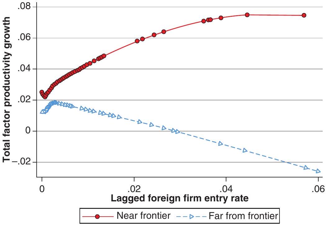
• Entry and entry threat enhance innovation and productivity growth among incumbents in sectors or countries that are initially close to the technological frontier, as the escape entry effect dominates in that case.

• Entry and entry threat reduce innovation and productivity growth among incumbents in sectors or countries that are far below the frontier, as the discouragement effect dominates in that case.

• Entry and entry threat enhance average productivity growth among incumbent firms when the threat has exceeded some threshold, but reduce average productivity growth among incumbents below that threshold. This is because as the probability \(p\) measuring the threat approaches unity, then almost all incumbents will be on the frontier, having either innovated or entered last period, and firms near the frontier respond to a further increase in \(p\) by innovating more frequently.

• Entry (and therefore, turnover) is growth-enhancing overall in the short run, because even in those sectors where incumbent innovation is discouraged by the threat of entry, the entrants themselves will raise productivity by implementing a frontier technology.

Figure 6.1, taken from Aghion et al. (2009), provides empirical support for the claim. The graph shows data for UK industries at the four-digit level. Firms are split as those close to the frontier and those away from the frontier (below the sample median for that industry). The level of competition is measured by the rate of foreign firm entry which is measured in the horizontal axis. The vertical axis shows subsequent productivity growth for domestic incumbents. As can be seen, close to the frontier entry accelerates growth. Further away it tends to slow it down.

Figure 6.1: Entry effects, from Aghion et al. (2009)

Interest groups as barriers to innovation

There’s another way in which monopolies can affect innovation. Imagine that monopolists use some of their profits to actually block the entry of new firms with better technologies - say, by paying off regulators to bar such entry. In fact, it may be a better deal than trying to come up with innovations! If that’s the case, then monopoly profits may actually facilitate the imposition of these barriers, by giving these monopolists more resources to invest in erecting barriers.

Monopolies are particularly dangerous in this regard, because they tend to be better able to act on behalf of their interests. Mancur Olson’s The Logic of Collective Action (2009) argues that policy is a recurrent conflict between the objectives of concentrated interest groups and those of the general public, for which benefits and costs are typically diffused. According to Olson, the general public has less ability to organise collective action because each actor has less at stake, at least relative to concentrated interest groups, which thus have the upper hand when designing policy. In short, monopolies have an advantage in organising and influencing policy. One implication of this logic is that the seeds of the decline of an economy are contained in its early rise: innovation generates rents that help the development of special-interest lobbies that can then block innovation. This is the argument raised by Mancur Olson, again, in his 1983 book The Rise and Decline of Nations (1983).

More recently, the theme of incumbents blocking innovation and development has been taken up by other authors. Parente and Prescott (1999) develop a model capturing this idea, and argue that the effects can be quantitatively large. Restricting the model so that it is consistent with a number of observations between rich and poor countries, they find that eliminating monopoly rights would increase GDP by roughly a factor of 3! Similarly, in their the popular book Why Nations Fail,

Acemoglu and Robinson (2012) argue, with evidence from a tour de force through history and across every continent, that the typical outcome is that countries fail to develop because incumbents block innovation and disruption.

6.3.3 Scale effects

The models of the previous section delivered a specific but fundamental result: scale effects. In other words, they predict that the growth rates will increase with the size of the population or markets. Intuitively, as we discussed, there are two sides to this coin. On the supply side, if growth depends on ideas, and ideas are produced by people, having more people means having more ideas. On the demand side, ideas are a fixed cost - once you produce a blueprint for a flying car, you can produce an arbitrary amount of flying cars using the same blueprint - and having a larger market enables one to further dilute that fixed cost.

The big question is: do the data support that prediction? Kremer (1993) argues that over the (very) long run of history the predictions of a model with scale effects are verified. He does so by considering what scale effects imply for population growth, which is determined endogenously in his model: population growth is increasing in population. He goes on to test this by checking that, using data from 1,000,000 B.C. to 1990, it does seem to be the case that population growth increases with population size. He also shows that, comparing regions that are isolated from each other (e.g. the continents over pre-modern history), those with greater population displayed faster technological progress.

This suggests that scale effects are present on a global scale, but that remains controversial. For instance, Jones (1995) argues that the data does not support the function in (6.2). For example, the number of scientists involved in R&D grew manifold in the post-World War II period without an increase in the rate of productivity growth. Instead, he argues that the evidence backs a modified version of the innovation production function, in which we would adapt (6.2) to look like this:

\[ \frac{\dot{M}}{M}=B Z_{M} M^{-\beta}, \tag{6.20}\]

with \(\beta>0\). This means that ideas have a diminishing return as you need more people to generate the same rate of innovation. In a world like this, research may deliver a constant rate of innovation (such as the so-called Moore’s law on the evolution of the processing capability of computers), but only due to substantially more resources devoted to the activity. This model leads to growth without scale effects, which Jones (1995) refers to as semi-endogenous growth.

It is also worth thinking about what scale effects mean for individual countries. Even if there are scale effects for the global economy, it seems quite obvious that they aren’t really there for individual countries: it’s not as if Denmark has grown that much slower than the U.S., relative to the enormous difference in size of the two economies. This can be for two reasons. First, countries are not fully isolated from each other, so the benefits of scale leak across borders. Put simply, Danish firms can have access to the U.S. market (and beyond) via trade. This immediately generates a potential connection between trade policy and growth, operating via scale effects. A second reason, on the flip-side, is that countries are not fully integrated domestically, i.e. there are internal barriers to trade that prevent countries from benefiting from their size. A paper by Ramondo et al. (2016) investigates the two possibilities, calibrating a model where countries are divided into regions, and find that the second point is a lot more important in explaining why the Denmarks of the world aren’t a lot poorer than the Indias and Chinas and U.S.

6.4 The future of growth

Are we headed to unprecedented growth? Or to stagnation?

The forces highlighted in these models of innovation, and their policy implications, have huge consequences for what we think will happen in the future when it comes to economic growth. There is a case for optimism, but also for its opposite.

Consider the first. If scale effects are present on a global scale, then as the world gets bigger growth will be faster, not the other way around. To see this, it is worth looking at the Kremer (1993) model in more detail, in a slightly simplified version. Consider the production function in

\[ Y=A p^{\alpha} T^{1-\alpha}=A p^{\alpha}, \tag{6.21}\]

where \(p\) is population and \(T\) is land which is available in fixed supply which, for simplicity, we will assume is equal to 1 . We can rewrite it as

\[ y=A p^{\alpha-1} . \tag{6.22}\]

The population dynamics have a Malthusian feature in the sense that they revert to a steady state that is sustainable given the technology. In other words, population adjusts to technology so that output per capita remains at subsistence level; as in the Malthusian framework, all productivity gains translate into a larger population, not into higher standards of living. (This is usually thought of as a good description of the pre-industrial era, as we will discuss in detail in Chapter 10.)

\[ p=\left(\frac{\bar{y}}{A}\right)^{\frac{1}{\alpha-1}} . \tag{6.23}\]

Critically, the scale effects come into the picture via the assumption that

\[ \frac{\dot{A}}{A}=p g . \tag{6.24}\]

i.e. the rate of technological progress is a function of world population, along the lines of the endogenous growth models we have seen. We can now solve for the dynamics of population, using (6.23) and then (6.24):

\[ \ln p=\left(\frac{1}{\alpha-1}\right)[\ln \bar{y}-\ln A], \tag{6.25}\]

\[ \frac{\dot{p}}{p}=-\left(\frac{1}{\alpha-1}\right) \frac{\dot{A}}{A}=\frac{1}{1-\alpha} \frac{\dot{A}}{A}=\frac{1}{1-\alpha} p g, \tag{6.26}\]

\[ \frac{\dot{p}}{p}=\left(\frac{g}{1-\alpha}\right) p . \tag{6.27}\]

In other words, population growth is increasing in population - which means that growth is explosive!

If true, this has enormous consequences for what we would expect growth to be in the future. For instance, if we think that both China and India have recently become much more deeply integrated into the world economy, can you imagine how many ideas these billions of people can come up with?

Can you fathom how much money there is to be made in developing new ideas and selling the resulting output to these billions of people? China and India’s integration into the world economy is an added boost to growth prospects on a global scale. In fact, as growth accelerates we may reach a point where machines take over in the accumulation of knowledge, making growth explode without bounds. (You may have heard of this being described as the singularity point.¹¹ )

Yet others have argued that, to the contrary, we are looking at a future of stagnation. Gordon (2018) argues that technological progress has so far relied on three main waves of innovation: the first industrial revolution (steam engine, cotton spinning, and railroads), the second industrial revolution (electricity, internal combustion engine, and running water), and the third industrial revolution (computers and the internet). He argues that the fruit of those waves has been reaped, and mentions a number of factors that may lead to lower future growth:

• The end of the demographic dividend. The process of absorption of women in the labour forces has ended, and the decline in birth rates further pushes down the growth of the labour force.

• Growth in education achievements also has been steadily declining as all the population achieves a minimum standard.

• The scope for growth via imitation falls as previous imitators reach the technological frontier.

• Climate change will require a reduction in future growth.

Some of these factors apply to a greater or lesser degree to other countries. China, for example, also faces a population challenge as its population ages at an unheard-of rate, and education levels have universally improved. At the same time, one might argue that the scope for imitation remains huge. Only assuming that all countries below average world income attain average world income in the next 100 years will deliver an extra \(2 \%\) growth in world GDP for the next 100 years. Time will tell, we suppose.

6.5 What have we learned?

In this chapter we presented models of technological innovation, but including technology as a factor of production implies increasing returns to scale, meaning that innovation has to be paid for in some way that cannot be simply via its marginal product. We tackled the issue in three steps. First, we modelled innovation as an increase in the complexity of the production function through a larger number of varieties. Second, as a process of improved quality in varieties which displace previous versions, we developed a framework more akin to Schumpeter’s idea of creative destruction. We saw that these two versions both highlight the importance of non-competitive behaviour, with monopoly profits driving the incentive to innovation. They also showcase scale effects: bigger market size implies faster innovation and growth because of the supply and demand for new ideas. In addition, the Schumpeterian version highlighted that there can be too much innovation and growth from a social perspective, as some of the incentive to innovate for private firms is simply to steal monopoly rents from incumbents without a counterpart in social welfare.

We then went over a number of policy issues, through the lens of the models of endogenous growth based on innovation. We saw that distance to the technological frontier can affect the incentives to innovate or imitate. We also saw that the relationship between competition and growth is more subtle than the basic model may indicate. Competition stimulates innovation for firms close to the frontier, but discourages innovation for firms farther away from the frontier. We then went over the debate on the extent to which scale effects matter in practice, presenting a number of arguments on both

directions. Finally, we briefly discussed an ongoing debate between those who believe growth will falter and those who think that growth will accelerate.

6.6 What next?

Acemoglu’s (2009) textbook on economic growth provides further details and nuances on the issues discussed here. You can also follow Acemoglu’s more recent work on automation. How would the world look if growth accelerates and, for example, robots become ubiquitous? Will this lead to pervasive unemployment? Will this lead to increased income inequality? This has been explored in Acemoglu and Restrepo (2017) and Acemoglu and Restrepo (2020).

In terms of innovation models, an excellent source is the classic Grossman and Helpman (1991) book. In our description of their models we have focused on the steady states, whereas there you will find a full description of the dynamics of the models discussed here. They also go into a lot more detail on the links between trade and economic growth, well beyond our discussion on market size and protection. Similarly, the book by Aghion and Howitt (2008) is a great starting point for further exploration of the Schumpeterian approach that the authors pioneered, and especially on the subtle interplay between competition and innovation. A more recent book by Aghion et al. (2021) also covers and develops these ideas in highly accessible fashion.

If you want more on the debate on the future of growth, the book by Gordon (2017) is a good starting point. That discussion is also the bread-and-butter of futurologists, among which Harari (2018) is a good example. It is interesting to read these books through the lenses of the endogenous growth models we have seen here.

References

Acemoglu, D. (2009). Introduction to modern economic growth. Princeton University Press.

Acemoglu, D., Aghion, P., & Zilibotti, F. (2006). Distance to frontier, selection, and economic growth. Journal of the European Economic Association, 4(1), 37-74.

Acemoglu, D. & Restrepo, P. (2017). Secular stagnation? The effect of aging on economic growth in the age of automation. American Economic Review, 107(5), 174-79.

Acemoglu, D. & Restrepo, P. (2020). Robots and jobs: Evidence from U.S. labor markets. Journal of Political Economy, 128(6), 2188-2244.

Acemoglu, D. & Robinson, J. A. (2012). Why nations fail: The origins of power, prosperity, and poverty. Currency.

Aghion, P., Blundell, R., Griffith, R., Howitt, P., & Prantl, S. (2009). The effects of entry on incumbent innovation and productivity. The Review of Economics and Statistics, 91(1), 20-32.

Aghion, P. & Howitt, P. (1990). A model of growth through creative destruction. National Bureau of Economic Research.

Aghion, P. & Howitt, P. (2006). Appropriate growth policy: A unifying framework. Journal of the European Economic Association, 4(2-3), 269-314.

Aghion, P. & Howitt, P. W. (2008). The economics of growth. MIT Press.

Gordon, R. J. (2017). The rise and fall of American growth: The U.S. standard of living since the Civil War. Princeton University Press.

Gordon, R. J. (2018). Why has economic growth slowed when innovation appears to be accelerating? National Bureau of Economic Research.

Grossman, G. M. & Helpman, E. (1991). Innovation and growth in the global economy. MIT Press.

Harari, Y. N. (2018). 21 lessons for the 21st century. Random House.

Jones, C. I. (1995). R & d-based models of economic growth. Journal of Political Economy, 103(4), 759-784.

Kremer, M. (1993). Population growth and technological change: One million B.C. to 1990. The Quarterly Journal of Economics, 108(3), 681-716.

Olson, M. (1983). The rise and decline of nations: Economic growth, stagflation, and social rigidities. Yale University Press.

Olson, M. (2009). The logic of collective action: Public goods and the theory of groups, second printing with a new preface and appendix. Harvard University Press.

Parente, S. L. & Prescott, E. C. (1999). Monopoly rights: A barrier to riches. American Economic Review, 89(5), 1216-1233.

Ramondo, N., Rodríguez-Clare, A., & Saborío-Rodríguez, M. (2016). Trade, domestic frictions, and scale effects. American Economic Review, 106(10), 3159-84.

Romer, P. M. (1990). Endogenous technological change. Journal of Political Economy, 98(5, Part 2), S71-S102.

Schumpeter, J. A. (1942). Capitalism. Socialism and democracy, 3, 167.

Williams, H. L. (2013). Intellectual property rights and innovation: Evidence from the human genome. Journal of Political Economy, 121(1), 1-27.

---

1. You may also notice the new exponent \(\frac{1}{\alpha}\), which will afford notational simplicity as we pursue the algebra.

2. This happens to be a property of the equilibrium of this model, and not an assumption, but we will simply impose it here for simplicity.

3. To see this, note that differentiating the term \(\left[\int_{0}^{M} X(i)^{\alpha} d i\right]^{\frac{1}{\alpha}}\) with respect to \(X(i)\) yields \(X(i)^{\alpha-1}\) \(\left[\int_{0}^{M} X(i)^{\alpha} d i\right]^{\frac{1-\alpha}{\alpha}}\), and \(\left[\int_{0}^{M} X(i)^{\alpha} d i\right]^{\frac{1-\alpha}{\alpha}}=1\) because of our normalisation to unit output.

4. Why is the denominator \(B Z_{M}+\rho\) the appropriate discount rate by which to divide \(\pi_{t}\) ? If \(\pi_{t}\) were constant, obtaining the present value of profits would require simply dividing it by the (constant) interest rate. But \(\pi_{t}\) is not constant: it grows at the rate at which \(\frac{w_{t}}{M_{t}}\) grows. Since wages must in equilibrium grow at the rate of output, it follows that \(\frac{w_{t}}{M_{t}}\) grows at the growth rate of output minus the growth rate of \(M_{t}: \frac{1-2 \alpha}{\alpha} B Z_{M}\). Subtracting this from the interest rate gives us the appropriate discount rate: \(B Z_{M}+\rho\).

5. We can use the consumer discount rate \(\rho\) because we assume firms are held in a diversified portfolio and there is no idiosyncratic risk.

6. Labour demand in production follows from this: each sector uses one unit of labor per unit of the good being produced. With total expenditure normalized to one, it follows that they sell \(x=\frac{1}{p}=\) \(\frac{1}{\text { lambdaw }}=\frac{\delta}{w}\) units each, which integrated between 0 and 1, for all sectors, yields the result.

7. Not quite the sum, but close enough. For those of you who are more mathematically inclined: define \(x_{i t} \equiv \log X_{i t}\) for any \(X\), then from (6.16) you can write \(y_{i t}=(1-\alpha) a_{i t}+\alpha k_{i t}\). Now assume the many sectors in the economy fall in the interval [0, 1], and integrate \(y_{i t}\) over that interval: \(\int_{0}^{1} y_{i t} d i=(1-\alpha) \int_{0}^{1} a_{i t}+\alpha \int_{0}^{1} k_{i t} \Rightarrow y_{t}=(1-\alpha) a_{t}+\alpha k_{t}\). Define \(Y_{t} \equiv \exp \left(y_{t}\right)\), and (6.17) follows. In sum, (6.17) essentially defines \(X_{t}=\exp \left(\left(\int_{0}^{1} \log X_{i t} d i\right)\right)\) for any variable \(X\). These are all monotonic transformations, so we are fine.

8. Williams (2013) shows an interesting piece of evidence: gene sequences subject to IP protection by private firm Celera witnessed less subsequent scientific research and product development, relative to those sequenced by the public Human Genome Project.

9. This is an insight that Schumpeter himself had pioneered in his book Capitalism, Socialism and Democracy, back in 1942. See Schumpeter (1942).

10. See https://www.monticello.org/site/research-and-collections/patents.

11. As in \(\frac{1}{x}\) when it approaches 0.