17 Fiscal policy I: Public debt and the effectiveness of fiscal policy
We have now reached the point at which we can use our hard-earned theoretical tools to study in depth the main policy instruments of macroeconomics, and eventually their long-run and short-run effects. We will start by considering fiscal policy, which means we will now address some of the most pressing policy questions in both developing and developed countries: does an increase in government expenditure increase output, or does it reduce it? What are the determinants of fiscal policy? What are the views?
Fiscal policy can always be thought of under two lights. On one level, it is a component of aggregate demand and will interest us as a tool of macroeconomic stabilisation; on the other hand, it also has a role in terms of determining the provision of public goods which brings in a whole host of other long-run considerations associated with the quality of that spending.
As a tool of macroeconomic stabilisation it is fundamentally different from monetary policy because fiscal policy requires resources, in other words, it needs to be financed. The result is that whatever expansion is obtained by fiscal spending will be diluted by the negative effect produced by the fact that it needs to obtain resources from the economy to finance itself. As a result it will always unavoidably put in motion a countervailing effect that must be taken into account.
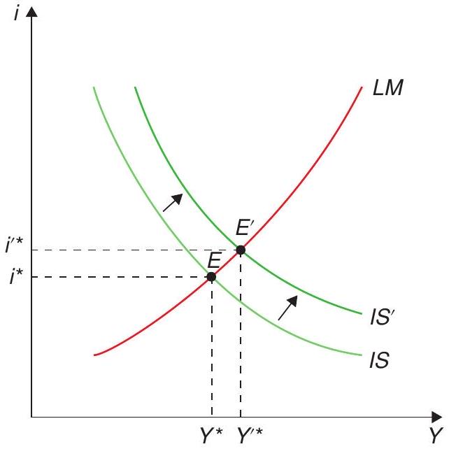
This chapter will deal with the first role of fiscal policy, its role for demand management, which happens to be where we typically have our first encounter with the topic at the undergraduate level. In fact, our treatment of fiscal policy illustrates how the things we learn in undergraduate-level macro can be misleading. For instance, in the traditional Keynesian rendition, fiscal policy helps stabilise output you may remember that an increase in G moves the IS to the right (see Figure 17.1). But this “undergraduate level” analysis is incomplete because it assumes that private consumption or investment are not affected by the increased expenditure. But how is the expenditure financed? Does this financing affect other components of aggregate demand? Imagine a permanent increase in expenditures financed with taxes. Our model of permanent income would anticipate a one to one decrease in private consumption, quite the opposite of a consumption function that is a rigid function of income.
In fact, if we ignore the financing side of the expenditure (be it through taxes or debt) it is evident that some budget constraint will be violated. Either the government is spending what it does not have, or consumers are spending what they cannot afford. Once we include the complete picture we realise that some variables need to adjust - but when does this occur? And how? And by how much? It is these issues that make the analysis of fiscal policy so complex.
We will thus start our analysis by considering the government’s intertemporal budget constraint. We have also explored the role of intertemporal budget constraints in analysing consumption and current account dynamics, the same analytical tools we used then will come in handy here. We will see the results that flow from this analysis in terms of the scope of fiscal policy and public debt dynamics.
17.1 The government budget constraint
We must recognise that the government cannot create resources out of nothing, so it must respect an intertemporal budget constraint. This entails that the present value of government spending is limited by the present value of taxes (minus initial debt).
Let us start by looking carefully at the government budget constraint. Let \(g_{t}\) and \(\tau_{t}\) denote the government’s real purchases and tax revenues at time \(t\), and \(d_{0}\), its initial real debt outstanding. The simplest definition of the budget deficit is that it is the rate of change of the stock of debt. The rate of change in the stock of real debt equals the difference between the government’s purchases and revenues, plus the real interest on its debt. That is,
\[ \dot{d}_{t}=\left(g_{t}-\tau_{t}\right)+r d_{t}, \tag{17.1}\]
where \(r\) is the real interest rate.
The term in parentheses on the right-hand side of (17.1) is referred to as the primary deficit. It is the deficit excluding interest payments of pre-existing debt, and it is often a better way of gauging how fiscal policy at a given time is contributing to the government’s budget constraint, since it leaves aside the effects of what was inherited from previous policies.
The government is also constrained by the standard solvency (no-Ponzi game) condition
\[ \lim _{T \rightarrow \infty}\left(d_{T} e^{-r T}\right) \leq 0 . \tag{17.2}\]
The government’s budget constraint does not prevent it from staying permanently in debt, or even from always increasing the amount of its debt. Recall that the household’s budget constraint in the Ramsey model implies that in the limit the present value of its wealth cannot be negative. Similarly, the restriction the budget constraint places on the government is that in the limit of the present value of its debt cannot be positive. In other words, the government cannot run a Ponzi scheme in which it raises new debt to pay for the ballooning interest on pre-existing debt. This condition is at the heart of the discussions on the solvency or sustainability of fiscal policy, and is the reason why sustainability exercises simply test that dynamics do not have government debt increase over time relative to GDP.
How do we impose this solvency condition on the government? We follow our standard procedure of solving the differential equation that captures the flow budget constraint. We can solve (17.1) by applying our familiar method of multiplying it by the integrating factor \(e^{-r t}\), and integrating between 0 and \(T\) :
\[ \begin{aligned} & \dot{d}_{e} e^{-r t}-r d_{t} e^{-r t}=\left(g_{t}-\tau_{t}\right) e^{-r t} \Rightarrow \\ & d_{T} e^{-r T}=d_{0}+\int_{0}^{T}\left(g_{t}-\tau_{t}\right) e^{-r t} d t . \end{aligned} \tag{17.3}\]
\[ \lim _{T \rightarrow \infty}\left(d_{T} e^{-r T}\right)=d_{0}+\int_{0}^{\infty}\left(g_{t}-\tau_{t}\right) e^{-r t} d t \leq 0, \tag{17.4}\]
Applying the solvency condition (17.2) and rearranging, this becomes
\[ \int_{0}^{\infty} g_{t} e^{-r t} d t \leq-d_{0}+\int_{0}^{\infty} \tau_{t} e^{-r t} d t \tag{17.5}\]
A household’s budget constraint is that the present value of its consumption must be less than or equal to its initial wealth plus the present value of its labour income. A government faces an analogous constraint: the present value of its purchases of goods and services must be less than or equal to its initial wealth plus the present value of its tax receipts. Note that because \(d_{0}\) represents debt rather than wealth, it enters negatively into the budget constraint.
An alternative way of writing this constraint is
\[ \int_{0}^{\infty}\left(\tau_{t}-g_{t}\right) e^{-r t} d t \geq d_{0} \tag{17.6}\]
Expressed this way, the budget constraint states that the government must run primary surpluses large enough in present value to offset its initial debt.
17.2 Ricardian equivalence
We add households to our problem, and derive a very important result in the theory of fiscal policy, namely Ricardian equivalence: given a path for government spending, it doesn’t matter whether it is financed via taxes or debt. We discuss the conditions under which this result holds, and the caveats to its application in practice.
Let us now add households to the story, and ask questions about the effects of fiscal policy decisions on private actions and welfare. In particular, for a given path of spending, a government can choose
to finance it with taxes or bonds. Does this choice make any difference? This question is actually at the heart of the issue of countercyclical fiscal policy. If you remember the standard Keynesian exercise, a fiscal stimulus is an increase in government spending that is not matched by an increase in current taxes. In other words, it is a debt-financed increase in spending. Is this any different from a policy that would raise taxes to finance the increased spending?
A natural starting point is the neoclassical growth model we have grown to know and love. To fix ideas, consider the case in which the economy is small and open, domestic agents have access to an international bond \(b\) which pays an interest rate \(r\) (the same as the interest rate on domestic government debt), and in which all government debt is held by domestic residents.
When there are taxes, the representative household’s budget constraint is that the present value of its consumption cannot exceed its initial wealth plus the present value of its after-tax labour income:
\[ \int_{0}^{\infty} c_{t} e^{-r t} d t=b_{0}+d_{0}+\int_{0}^{\infty}\left(y_{t}-\tau_{t}\right) e^{-r t} d t \tag{17.7}\]
Notice that initial wealth now apparently has two components: international bond-holdings \(b_{0}\) and domestic public debt holdings \(d_{0}\).
17.2.1 The effects of debt vs tax financing
Breaking the integral on the right-hand side of (17.7) in two gives us
\[ \int_{0}^{\infty} c_{t} e^{-r t} d t=b_{0}+d_{0}+\int_{0}^{\infty} y_{t} e^{-r t} d t-\int_{0}^{\infty} \tau_{t} e^{-r t} d t \tag{17.8}\]
It is reasonable to assume that the government satisfies its budget constraint, (17.5), with equality. If it did not, its wealth would be growing forever, which does not seem realistic. With that assumption, (17.5) implies that the present value of taxes, \(\int_{t=0}^{\infty} \tau_{t} e^{-r t} d t\), equals initial debt \(d_{0}\) plus the present value of government purchases, \(\int_{t=0}^{\infty} g_{t} e^{-r t} d t\). Substituting this fact into (17.8) gives us
\[ \int_{0}^{\infty} c_{t} e^{-r t} d t=b_{0}+\int_{0}^{\infty} y_{t} e^{-r t} d t-\int_{0}^{\infty} g_{t} e^{-r t} d t \tag{17.9}\]
Equation (17.9) shows that we can express the households’ budget constraint in terms of the present value of government purchases without any reference to the division of the financing of those purchases at any point in time between taxes and bonds. Since the path of taxes does not enter either households’ budget constraint or their preferences, it does not affect consumption. Thus, we have a key result: only the quantity of government purchases, not the division of the financing of those purchases between taxes and bonds, affects the economy. This was first pointed out by British economist David Ricardo, back in the 19th century, which is why it is called Ricardian equivalence. Barro (1974) revived this result, proving it in the context of the NGM.
To see the point more starkly, focus on the case in which the agent maximises
\[ \int_{0}^{\infty} u\left(c_{t}\right) e^{-\rho t} d t \tag{17.10}\]
where \(\rho>0\) is the rate of time preference. Assume moreover that \(r=\rho\), as we have done in the past. This implies that the optimal consumption path is flat:
\[ c_{t}=c \text { for all } t \geq 0 . \tag{17.11}\]
Applying this to (17.9) yields
\[ c=r b_{0}+r \int_{0}^{\infty} y_{t} e^{-r t} d t-r \int_{0}^{\infty} g_{t} e^{-r t} d t \tag{17.12}\]
so that consumption is equal to permanent income. Again, since the path of taxes does not enter the RHS of (17.12), it does not affect consumption.
What is the intuition for this remarkable result? If a certain amount of spending is financed by issuing debt, the solvency condition implies that this debt must be repaid at some point. In order to do so, the government will have to raise taxes in the exact present value of that spending. This means that government bonds are not net wealth: for a given path of government expenditures, a higher stock of debt outstanding means a higher present value of taxes to be paid by households. In other words, the government cannot create resources out of nothing, it can only transfer them over time; rational, forward-looking consumers recognise this, and do not change their behaviour from what it would have been had that spending been financed with taxes immediately.
17.2.2 Caveats to Ricardian equivalence
This very strong result was obtained under rather stringent assumptions, which we now underscore:
Consumers live forever, so that a change in taxes even very far away in time matters to them. But note, if consumers had finite lives but acted altruistically in regards their sons and daughters, the result would still hold. This was the insight of Barro (1974).
Taxes are lump-sum and therefore non-distortionary. If the present value of private income \(\int_{0}^{\infty} y_{t} e^{-r t} d t\), for instance, fell if taxes increased (due to distortionary effects on investment or labour supply), then Ricardian equivalence would not hold.
Consumers face no borrowing constraints so that all they care about is the present value of taxes. Consider, by contrast, an agent who cannot borrow and who has no initial wealth. Then, a tax increase today that was perfectly offset (in present value terms) by a tax break \(T\) periods later would reduce his income today - and therefore his consumption today- regardless of what happened in the future.
Agents and the government can borrow at the same rate of interest \(r\). If government could borrow more cheaply than consumers, for instance, by cutting taxes and running a larger deficit today, it would increase the wealth of consumers, enabling them to increase their consumption.
17.3 Effects of changes in government spending
We show that changes in government spending have real effects, and that they are very different depending on whether they are temporary or permanent. Permanent increases are matched one-forone by decreases in consumption. Temporary increases are matched less than one-for-one, with a current account deficit emerging as a result.
Now ask the opposite question. What is the effect of changes in government spending on consumption, savings, and the current account of the economy?
To get started, notice that the private budget constraint is
\[ \dot{b}_{t}+\dot{d}_{t}=r\left(b_{t}+d_{t}\right)+y_{t}-\tau_{t}-c_{t} . \tag{17.13}\]
Combining this with the government budget constraint (17.1) we have
\[ \dot{b}_{t}=r b_{t}+y_{t}-g_{t}-c_{t} . \tag{17.14}\]
Suppose now that income is constant throughout, but government consumption can vary. In particular, suppose that \(g_{t}\) can take two values: \(g^{H}\) and \(g^{L}\), with \(g^{H}>g^{L}\). To gain further insights, we study the effects of permanent and temporary changes in government spending that take place at time 0.
17.3.1 The initial steady state
Assume that just prior to the shock, spending is expected to remain constant forever; that is, \(g_{t}=g^{L}\) for all \(t\). The economy is thus in a steady state in which consumption is given by
\[ c=r b_{0}+y-g^{L} . \tag{17.15}\]
In the initial steady state, the current account is zero.
17.3.2 Permanent increase in government spending
Suppose now that at time 0 there is an unanticipated and permanent increase in spending from \(g^{L}\) to \(g^{H}\). From (17.12) it follows that consumption adjusts instantaneously to its new (and lower) value:
\[ c^{\prime}=r b_{0}+y-g^{H}, \quad t \geq 0 . \tag{17.16}\]
Since consumption falls one-to-one with government spending, the trade and current accounts do not change. Hence, an unanticipated and permanent increase in spending has no impact on the current account.
17.3.3 Temporary increase in spending
Suppose that the economy is in the initial steady state described above, with consumption given by (17.15). At time 0 , there is an unanticipated and temporary increase in spending:
\[ g_{t}= \begin{cases}g^{H}, & 0 \leq t<T \\ g^{L}, & t \geq T,\end{cases} \tag{17.17}\]
for some \(T>0\).
First compute the consumption path. From (17.12) it follows that consumption falls immediately to the level given by
\[ c^{\prime \prime}=r b_{0}+y-g^{H}\left(1-e^{-r T}\right)-g^{L} e^{-r T}, \quad t \geq 0 . \tag{17.18}\]
Next compute the current account path. Plugging (17.18) into (17.14) we have
\[ \dot{b}_{t}=r\left(b_{t}-b_{0}\right)+\left(g^{L}-g^{H}\right) e^{-r T}, \quad 0 \leq t<T . \tag{17.19}\]
Notice that at time \(t=0\) this implies
\[ \dot{b}_{0}=\left(g^{L}-g^{H}\right) e^{-r T}<0 . \tag{17.20}\]
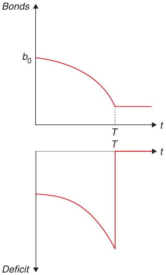
The current account is negative \(\left(\dot{b}_{0}<0\right)\) from the start. It follows that \(b_{t}-b_{0}<0\), and, from (17.19), that \(\dot{b}_{t}<0\) for all times between 0 and \(T\). The current account worsens over time and then jumps back to zero at time \(T\). Figure 17.2 shows the trajectory of the deficit and foreign assets in response to this temporary shock.
How do we know that the current account goes to 0 at time \(T\) ? Recall the current account is given by
\[ \dot{b}_{t}=r b_{t}+y_{t}-g_{t}-c_{t} . \tag{17.21}\]
Solving this for a constant path of income, spending, and consumption we have
\[ b_{T} e^{-r T}=b_{0}+\left(1-e^{-r T}\right)\left(\frac{y-g^{H}-c^{\prime \prime}}{r}\right) . \tag{17.22}\]
Plugging (17.18) into this expression we have
\[ r b_{T}=r b_{0}+\left(1-e^{-r T}\right)\left(g^{L}-g^{H}\right) . \tag{17.23}\]
Evaluating (17.14) at time \(T\) we have
\[ \dot{b}_{T}=r b_{T}+y-g^{L}-c^{\prime \prime} . \tag{17.24}\]
Finally, using (17.18) and (17.23) in (17.24), we obtain
\[ \begin{aligned} \dot{b}_{T}= & r b_{0}+\left(1-e^{-r T}\right)\left(g^{L}-g^{H}\right)+y-g^{L} \\ & -r b_{0}-y+g^{H}\left(1-e^{-r T}\right)+g^{L} e^{-r T} \end{aligned} \tag{17.25}\]
\[ = 0 . \tag{17.26}\]
That is, the current account is zero at time \(T\).
The key policy lesson of this discussion is that consumption does not fully offset the changes in government consumption when those changes are transitory. So, if government expenditure aims at changing aggregate demand, it has a much higher chance of achieving that objective if it moves in a transitory fashion. Here the excess spending affects the current account which can easily be governed by temporary changes in fiscal policy. This is why you may often hear mentions of twin deficits in policy debates, in reference to the idea that fiscal deficits can be accompanied by current account deficits.
17.4 Fiscal policy in a Keynesian world
We go over how fiscal policy fits into the (New) Keynesian framework. When there is the possibility of increasing output via aggregate demand (that is, in the short run), fiscal policy can affect output. That depends, however, on the consumer and firm responses, which take into account the budget constraints.
We have seen that, once we consider the government’s budget constraint, and its interaction with the households’ budget constraint, the effects of fiscal policy are radically modified, compared to what you may have been used to in undergraduate discussions.
As a starter, the effectiveness of fiscal policy as a tool for managing aggregate demand, in a full employment economy, is clearly dubious. For example, think about the NGM in a closed economy. It should be immediately clear that government spending cannot have an effect on output from the demand side: the government cannot through aggregate management increase the productive capacity of the economy, and this means its increased spending must crowd out something else. (In a small open economy model, as we have seen, it crowds out mostly consumption; in a closed or large open economy, it would also crowd out investment.) This has the flavour of Ricardian equivalence.
Having said that, we are still left with the question: where is the role for Keynesian fiscal policy? Is the conclusion that such policy is impossible? Not quite. Recall that the models so far in this chapter had no room for aggregate demand policy by assumption: the economies we’ve seen were not demand constrained and output was exogenous. In other words, one might think of them as descriptions of long-term effects. However, in a recession, the government can try to engage those that are sitting idle because of insufficient aggregate demand. This is the view that lies behind the thinking of proponents of fiscal stimulus.
To think more systematically about this, let us look at the role of government in the context of the canonical (discrete-time) New Keynesian model we saw in Chapter 15. The key change that we incorporate is to include government spending, which (in a closed economy) entails the following resource constraint:
\[ Y_{t}=C_{t}+G_{t} . \tag{17.27}\]
Expressing this in terms of (percentage) deviations from the steady state, it is easy to see that the log-linearised resource constraint is1
\[ \hat{y}_{t}=(1-\gamma) \hat{c}_{t}+\gamma \hat{g}_{t}, \tag{17.28}\]
where \(\gamma=\frac{\bar{G}}{\bar{Y}}\) is the steady state share of government spending, and the hat above a variable \(z\) represents log deviations from the steady state: \(\hat{z}_{t}=z_{t}-\bar{z}_{t}\).
Now take the Euler equation coming from consumer optimisation. Log-linearising around the (non-stochastic) steady state of the economy (and leaving aside the term in the discount rate \(\rho\), for
notational simplicity) yields our familiar
\[ \hat{c}_{t}=E_{t} \hat{c}_{t+1}-\sigma r_{t} . \tag{17.29}\]
Now, we can’t simply substitute output for consumption, as we did back in Chapter 15. Instead, substituting the new linearised resource constraint into (17.29) yields, after some simple manipulation.2
\[ \hat{y}_{t}=E_{t} \hat{y}_{t+1}-\sigma(1-\gamma)\left(i_{t}-E_{t} \pi_{t+1}-r_{g}^{n}\right), \tag{17.30}\]
where \(r_{g}^{n}=-\frac{\gamma}{\sigma(1-\gamma)} \Delta \hat{g}_{t+1}\). This term \(r_{g}^{n}\) is the modified version of the natural interest rate - that is to say, the rate that would keep output stable - that we encountered in Chapter 15.3 It is easy to see that a transitory increase in \(\hat{g}_{t}\) corresponds to an increase in that natural interest rate. In other words, a transitory fiscal expansion increases aggregate demand.
Here’s where you may ask: but isn’t the resource constraint being violated? Well, no: we have used (17.28) explicitly in our derivation, after all. The trick is that the resource constraint embodies the possibility that output itself is not fixed (in the short run), but can increase. That is the key distinction that allows for a potential effect of fiscal policy on aggregate demand.
Does that mean that an increase in government spending will lead to an increase in output? Not necessarily.
First, consumption will change as well. Note that the Euler equation that underpins the NKIS in (17.29) does not pin down the full consumption path: for that we must incorporate the intertemporal budget constraint. And we know that an increase in government spending must correspond to an increase in taxes at some point, and consumers will respond to that. In particular, in a Ricardian world, that response will be a one-for-one decrease in consumption if the increase is permanent, thereby negating the impact of government spending on aggregate demand. That a permanent increase in \(g\) has no effect on aggregate demand can be seen by noticing that a permanent increase in \(g\) will not change \(r_{g}^{n}\) in (17.30). That permanent changes in \(g\) have no effect may come as a surprise, given what it typically portrayed in intermediate texts, but on a simple inspection is obvious. Countries differ radically in the amount of government expenditures, but there is no relation between aggregate demand, recessions, or macroeconomic performance between them. Permanent changes in government spending just crowd out other components of aggregate demand.
More generally, the impact of government spending on aggregate demand is thus predicated on it being temporary, or on departures from Ricardian assumptions, as we have discussed.
On top of that, there is also a supply-side effect, via the behaviour of firms: the New Keynesian Phillips Curve (NKPC) will also be affected. You will recall that the NKPC looks like this:
\[ \pi_{t}=\beta E_{t} \pi_{t+1}+\kappa \hat{y}_{t} . \tag{17.31}\]
A shock to government spending will also have a supply-side effect via an increase in the output gap, thus affecting inflation expectations, which will feed back into the NKIS. In short, the fiscal multiplier that is, the change in output in response to a change in government spending - will depend on the specification and parameters of the model.
Finally, the NKIS makes it clear that this will depend on the response of monetary policy - and remember, the full specification of the canonical New Keynesian DSGE model requires the specification of a monetary policy rule. For instance, if monetary policy responds by increasing the nominal interest rate, it undoes the impact of fiscal expansion.
Summing up, our point is that to assess the role of fiscal policy it’s important to keep in mind that people will react to policy, and will consider (to a smaller or greater extent) its dynamic effects. Part of a fiscal stimulus will end up being saved to face future taxes, and the extent to which this will crowd out other sources of demand will depend on how demand-constrained the economy is. It must also take into account its effects on the perceived sustainability of current fiscal policies, as well as the response of monetary policy. All of these are empirical debates that take place, at least to some extent, within the context of this framework we’ve discussed. Let’s finish our discussion by considering what happens in practice.
17.4.1 The current (empirical) debate: Fiscal stimulus and fiscal adjustment
With all of these different effects in mind, we can look at some of the evidence regarding the effectiveness of fiscal policy and, closely related, on the implications of the kind of fiscal adjustment that might be needed in the face of soaring debt ratios.
The question on the effectiveness of fiscal policy as a tool for aggregate demand management is often subsumed in the discussion on the size of the multiplier: if I increase government spending a given amount, by what multiple of this amount will it increase output? The undergraduate text provides an unambiguous answer to this question: it goes up. But our model has led us to think of a number of things that might affect that multiplier: whether the increase is permanent or temporary and how agents react to it, the context in which it takes place, and what it entails for the future path of spending. There is a wide range of beliefs about that in the policy debate - as illustrated by the many countries in which proponents of fiscal expansion or austerity are pitched against one another. In practice, it is very hard to isolate that impact since there can obviously be reverse causality, and there are always lots of other things, besides the change in fiscal policy, that are going on at the same time and can also affect output. In sum, we have a classic identification challenge.
There are two main approaches to overcome that challenge. First, some people (e.g. Blanchard and Perotti 2002 and Ilzetzki et al. 2013) use what is called a structural vector autoregression (SVAR) econometric technique, which basically relies on the assumption that it takes time for fiscal policy to respond to news about the state of the economy. It uses VAR (regressing a vector of variables on their lags, essentially) to tease out predictable responses of fiscal policy to output and vice-versa, and attributes any correlation between the unpredicted components to the impact of government spending on output. The problem, of course, is that what is unpredicted by the econometrician need not be so for the agents themselves, so we can never be sure we’re estimating the true impact. The second approach is to use natural experiments where government spending increases due to some credibly exogenous factor. A popular example is wars and associated military buildups (e.g. Ramey and Shapiro 1999, Ramey 2009, Barro and Redlick 2011), and, on a similar note, a recent paper by Nakamura and Steinsson (2014) looks at the differential effect of military buildup shocks across U.S. regions. (Another example, from Shoag (2013), uses variation induced by changes in state pension fund returns.) The problem is that exercises rely on specific sources of spending that may not be typical. In other words, it’s hard to assess the external validity of these natural experiments.
The variation in the estimates is enormous. In the natural experiment literature, they range from 0.5 to 1.5, from military buildups, and reach above 2 in other approaches. The SVAR literature has wildly divergent numbers across time and countries and specific structural assumptions, ranging from -2.3 to 3.7! One state-of-the-art attempt, Ilzetzki et al. (2013), who use better (quarterly) data for a number of countries, also reached nuanced conclusions: (i) Short-run multiplier is negative
in developing countries; (ii) Multiplier is zero or negative when debt level is high; (iii) Multiplier is zero under flexible exchange rates, but positive under fixed exchange rates, and is higher in closed economies than in open economies. Note that (i) and (ii) are quite consistent with the effects we have been talking about: if people believe that higher spending is unsustainable, they would expect higher taxes in the near future, dampening the effect of the expansion. By the same token, (iii) is consistent with a simple Mundell-Fleming model, which we haven’t talked about in the book, but which you may recall from undergraduate macro: under flexible exchange rates, more government spending leads to a currency appreciation, which leads to a reduction in net exports that undoes the fiscal stimulus. These results share the flavour with our previous discussion of Ricardian equivalence: when deficits and debt levels become large, consumer behaviour seems to more clearly undo the effects of fiscal policy.
Of course, in practice, policymakers have to act even with all this uncertainty. Here’s an example, Table 17.1, shows the estimates generated by the non-partisan Congressional Budget Office (CBO) for the impact of the 2009 stimulus in the U.S. One can see patterns that are broadly in line with our discussion: (temporary) spending has a larger effect than tax cuts, tax cuts to people who are more likely to be credit-constrained have a larger effect. (Note that this short-term estimate keeps at a minimum the possible supply-side effects that might come from distortionary taxation. We will get to this in the next chapter.)
This discussion on the effectiveness of fiscal policy also colours the debate on the desirability and implications of fiscal adjustments aimed at putting the debt situation under control. As discussed in Alesina et al. (2019), the conventional wisdom that these adjustments would necessarily be contractionary is too simplistic. The inherent intertemporal nature of fiscal policy sees to that: maybe a fiscal contraction, by convincing people that a previously unsustainable debt trajectory is now sustainable, will “crowd in” private spending, as people anticipate lower taxes (or no tax hikes) in the future. It may also have the supply-side effects that will be the focus of our next chapter.
The evidence in Alesina et al. (2019) suggests that, in practice, many fiscal contractions have indeed been expansionary! It seems that this is particularly likely if the adjustment is about cutting spending rather than increasing taxes - perhaps because the former are deemed to be more sustainable in the long run. While there is controversy about the evidence - who would have thought? (see Ball et al. (2013), particularly with respect to what is selected as an episode of major fiscal contraction) - the point remains that the practice is more complex than what the simple undergraduate textbook view would have suggested.
17.5 What have we learned?
The key lesson from this chapter is that evaluating the macroeconomic impact of fiscal policy requires considering its dynamic implications and the existence of budget constraints. The fact that economic agents understand that means that any change in fiscal policy will meet with a response from the private sector, which in turn immediately affects the impact of that change.
The first expression of this logic is the Ricardian equivalence result: it does not matter whether a certain path of spending is financed via debt or taxes, because in the end it all has to come from taxes at some point. As a result, changes in government spending create a counteracting adjustment in private spending, because of future taxes. The size of the adjustment depends on whether the change is permanent or temporary - in the later case, the adjustment by consumption is less than one-for-one, and aggregate demand moves accordingly.
| Estimated Output Multipliers and Budgetary Costs of Major Provisions of the American Recovery and Reinvestment Act | ||||
|---|---|---|---|---|
| Type of Activity | Estimated Output Multipliers \({ }^{\mathbf{a}}\) | Major Provisions of ARRA | Total Budgetary Cost of Provisions, 2009-2019 \({ }^{\text {b }}\) | |
| Low Estimate | High Estimate | |||
| Purchases of Goods and Services by the Federal Government | 1.0 | 2.5 | Division A, Title II: Other; Title IV: Energy Efficiency and Renewable Energy; Title IV: Innovative Technology Loan Guarantee Program; Title IV: Other Energy Programs; Title V: Federal Buildings Fund; Title VIII: National Institutes of Health; Title VIII: Other Department of Health and Human Services | $88 billion |
| Transfer Payments to State and Local Governments for Infrastructure | 1.0 | 2.5 | Division A, Title VII: Clean Water and Drinking Water State Revolving Funds; Title XI: Other Housing Assistance; Title XII: Highway Construction; Title XII: Other Transportation | $44 billion |
| Transfer Payments to State and Local Governments for Other Purposes | 0.7 | 1.9 | Division A, Title VIII: Education for the Disadvantaged; Title VIII: Special Education; Title IX: State Fiscal Stabilization Fund; Division B, Title V: State Fiscal Relief Fund | $215 billion |
| Transfer Payments to Individuals | 0.8 | 2.2 | Division A, Title I: Supplemental Nutrition Assistance Program; Title VIII: Student Financial Assistance; Division B, Title II: Unemployment Compensation; Title III: Health Insurance Assistance | $100 billion |
| One-Time Payments to Retirees | 0.2 | 1.2 | Division B, Title II: Economic Recovery Payments, Temporary Aid to Needy Families, and Child Support \({ }^{\mathrm{c}}\) | $18 billion |
| Two-Year Tax Cuts for Lower- and MiddleIncome People | 0.5 | 1.7 | Division B, Title I: Refundable Tax Credits; Making Work Pay Credit; \({ }^{\mathrm{d}}\) American Opportunity Tax Credit \({ }^{\mathrm{d}}\) | $168 billion |
| One-Year Tax Cut for Higher-Income People | 0.1 | 0.5 | Increase in Individual AMT Exemption Amount \({ }^{\text {d }}\) | $70 billion |
| Extension of First-Time Homebuyer Credit | 0.2 | 1.0 | Extension of First-Time Homebuyer Credit \({ }^{\mathrm{d}}\) | $7 billion |
Still, we saw that fiscal policy can affect output in the short run, in a Keynesian world. But even in this case, understanding the impact of fiscal policy requires thinking about the private sector adjustments - driven by the shadow of the intertemporal budget constraints - as well as the response of monetary policy.
17.6 What next?
If you are interested in learning more about the debate on the impact of fiscal policy, a great starting point is the book Fiscal Policy After The Financial Crisis, edited by Alesina and Giavazzi (2013). It contains a thorough overview of different perspectives in that debate.
17.7 Appendix
17.7.1 Debt sustainability
Let us now turn to some practical issues when analysing fiscal policy from a dynamic perspective. Our discussion in this chapter has talked about how fiscal policy has to fit into an intertemporal budget constraint. But that raises the question: how do we know, in practice, whether a certain fiscal trajectory fits into the intertemporal budget constraint? If it does not we say the debt level is unsustainable, and we must expect some sort of change. We deal with this issue first. We then turn to some problems related to measurement, which are particularly important given the inherently dynamic nature of fiscal policy.
17.7.2 A simplified framework
An important issue in macroeconomic analysis is to figure out if the debt dynamics are sustainable. Strictly speaking, sustainability means satisfying the NPG condition: the present discounted value of debt in the long run has to be zero. This restriction is relatively imprecise as to short term debt dynamics. Debt can grow, and grow very fast, and still satisfy the NPG condition. There is an ample literature on this, but a very practical, though primitive, way of answering this question is by asking whether the debt-to-GDP ratio is increasing or not. According to this stark definition debt sustainability is achieved when the debt-to-GDP ratio is constant or declining over time.
With this in mind a typical debt sustainability analysis would start with the dynamic equation for debt:
\[ D_{t}=\left(1+r_{t}\right) D_{t-1}+(\overbrace{G_{t}-T_{t}}^{\text {primary deficit }}) . \tag{17.32}\]
(Note that this is the discrete-time equivalent of (17.1).) Divide this by \(G D P_{t}\) (we also multiply and divide the first term to the right of the equal sign by \(G D P_{t-1}\) ) to obtain
\[ \frac{D_{t}}{G D P_{t}}=\left(1+r_{t}\right) \frac{D_{t-1}}{G D P_{t-1}} \frac{G D P_{t-1}}{G D P_{t}}+\left(\frac{G_{t}}{G D P_{t}}-\frac{T_{t}}{G D P_{t}}\right) . \tag{17.33}\]
Denoting with lower cases the variables relative to GDP, the above becomes
\[ d_{t}=\frac{\left(1+r_{t}\right)}{(1+\gamma)} d_{t-1}+(\underbrace{g_{t}-t_{t}}_{p d_{t}}) \tag{17.34}\]
or
\[ d_{t}=\frac{\left(1+r_{t}\right)}{(1+\gamma)} d_{t-1}-(\underbrace{t_{t}-g_{t}}_{p s_{t}}), \]
where \(p d\) and \(p s\) stand for primary deficit and surplus (again, the difference between government expenditure and income, and vice versa, respectively, prior to interest payments), \(\gamma\) is the growth rate of GDP. Assume that we are in a steady state such that everything is constant. In this case
\[ d=\frac{(1+r)}{(1+\gamma)} d-p s, \tag{17.35}\]
which can be solved for the primary surplus needed for debt to GDP ratios to be stable:
\[ p s=d\left[\frac{(1+r)}{(1+\gamma)}-1\right]=d\left[\frac{1+r-1-\gamma}{1+\gamma}\right]=d\left[\frac{r-\gamma}{1+\gamma}\right] . \tag{17.36}\]
Any surplus larger than that in (17.36) will also do. In order to make this equation workable, practitioners typically try to estimate expected growth in the medium term (growth has to be assessed in the same denomination of the debt, so if debt is, say, in U.S. dollars, you should use the growth rate of GDP in current U.S. dollars), the interest rate can be estimated from the average interest payments, and debt to GDP ratios are typically available. Table 17.2 makes this computation for a series of values of \(g\) and \(d\) given a specific \(r\) (in this table we use 7%).
The table shows the primary surplus required to stabilise the debt to GDP ratio. It can also be used to estimate restructuring scenarios. Imagine a country (Greece?) with a debt to GDP ratio of \(150 \%\) and an expected growth rate of \(2 \%\). The table suggests it needs to run a budget surplus of \(7.6 \%\) of GDP. If only a \(2.5 \%\) surplus is feasible debt, sustainability obtains (at this interest rate) if debt is \(50 \%\) of GDP. To obtain debt sustainability the country needs a haircut of \(66 \%\).
Recent models have emphasized the stochastic nature of fiscal revenues and expenditures. Simulating these processes, rather than estimating a single number, they compute a distribution function for fiscal results thus allowing to compute the value at risk in public debt.
17.8 Measurement issues
The government budget constraint (17.5) involves the present values of the entire paths of purchases and revenues, and not the deficit at a point in time. As a result, conventional measures of either the primary or total deficit can be misleading about the real evolution of fiscal accounts. We illustrate this with three examples.
| Public debt to GDP (%) | GDP growth rate (%) | |||||
|---|---|---|---|---|---|---|
| 1 | 2 | 3 | 4 | 5 | 6 | |
| 35 | 2.1 | 1.7 | 1.4 | 1.0 | 0.7 | 0.3 |
| 40 | 2.4 | 2.0 | 1.6 | 1.2 | 0.8 | 0.4 |
| 45 | 2.7 | 2.2 | 1.7 | 1.3 | 0.9 | 0.4 |
| 50 | 3.0 | 2.5 | 1.9 | 1.4 | 1.0 | 0.5 |
| 55 | 3.3 | 2.7 | 2.1 | 1.6 | 1.0 | 0.5 |
| 60 | 3.6 | 2.9 | 2.3 | 1.7 | 1.1 | 0.6 |
| 65 | 3.9 | 3.2 | 2.5 | 1.9 | 1.2 | 0.6 |
| 70 | 4.2 | 3.4 | 2.7 | 2.0 | 1.3 | 0.7 |
| 75 | 4.5 | 3.7 | 2.9 | 2.2 | 1.4 | 0.7 |
| 80 | 4.8 | 3.9 | 3.1 | 2.3 | 1.5 | 0.8 |
| 85 | 5.0 | 4.2 | 3.3 | 2.5 | 1.6 | 0.8 |
| 90 | 5.3 | 4.4 | 3.5 | 2.6 | 1.7 | 0.8 |
| 95 | 5.6 | 4.7 | 3.7 | 2.7 | 1.8 | 0.9 |
| 100 | 5.9 | 4.9 | 3.9 | 2.9 | 1.9 | 0.9 |
| 110 | 6.5 | 5.4 | 4.3 | 3.2 | 2.1 | 1.0 |
| 120 | 7.1 | 5.9 | 4.7 | 3.5 | 2.3 | 1.1 |
| 130 | 7.7 | 6.4 | 5.0 | 3.8 | 2.5 | 1.2 |
| 140 | 8.3 | 6.9 | 5.4 | 4.0 | 2.7 | 1.3 |
| 150 | 8.9 | 7.4 | 5.8 | 4.3 | 2.9 | 1.4 |
| 160 | 9.5 | 7.8 | 6.2 | 4.6 | 3.0 | 1.5 |
17.8.1 The role of inflation
The first example is the effect of inflation on the measured deficit. The change in nominal debt outstanding - that is, the conventionally measured budget deficit - equals the difference between nominal purchases and revenues, plus the nominal interest on the debt. If we let \(D\) denote the nominal debt, the nominal deficit is thus
\[ \dot{D}_{t}=P_{t}\left(g_{t}-\tau_{t}\right)+i_{t} D_{t}, \tag{17.37}\]
where \(P\) is the price level and \(i\) is the nominal interest rate. When inflation rises, the nominal interest rate rises for a given real rate. Thus, interest payments and the deficit increase. Yet the higher interest payments are just offsetting the fact that the higher inflation is eroding the value of debt. The behaviour of the real stock of debt, and thus the government’s budget constraint is not affected.
To see this formally, we use the fact that, by definition, the nominal interest rate equals the real rate plus inflation. This allows us to rewrite our expression for the nominal deficit as
\[ \dot{D}_{t}=P_{t}\left(g_{t}-\tau_{t}\right)+\left(r+\pi_{t}\right) D_{t} . \tag{17.38}\]
Dividing through by \(P_{t}\) this yields
\[ \frac{\dot{D}_{t}}{P_{t}}=g_{t}-\tau_{t}+\left(r+\pi_{t}\right) \frac{D_{t}}{P_{t}} . \tag{17.39}\]
Next define real debt as
\[ d_{t}=\frac{D_{t}}{P_{t}}, \tag{17.40}\]
so that (17.39) becomes
\[ \frac{\dot{D}_{t}}{P_{t}}=g_{t}-\tau_{t}+\left(r+\pi_{t}\right) d_{t} . \tag{17.41}\]
But recall next from (17.1) that
\[ \dot{d}_{t}=g_{t}-\tau_{t}+r d_{t} . \tag{17.42}\]
Using this in (17.41) we finally have
\[ \frac{\dot{D}_{t}}{P_{t}}=\dot{d}_{t}+\pi_{t} d_{t} . \tag{17.43}\]
Higher inflation raises the conventional (nominal) measure of the deficit even when it is deflated by the price level. This was Brazil’s problem for many years.
17.8.2 Asset sales
The second example is the sale of an asset. If the government sells an asset, it increases current revenue and thus reduces the current deficit. But it also forgoes the revenue the asset would have generated in the future. In the natural case where the value of the asset equals the present value of the revenue it will produce, the sale has no effect on the present value of the government’s revenue. Thus, the sale affects the current deficit but does not affect the government’s net worth. It follows that the effect of privatisation on the fiscal position of the government has to be analysed carefully, as it is not given by the bump in measured current revenue. If there is a positive impact it should be predicated on the idea that the present value of the revenues to the private sector is greater than what would be the case for the government (say, because the government runs it inefficiently), so that the buyer would be willing to pay more than the present value of the revenues the government would obtain from it. But this argument, not to speak of the computation, is seldom done.
17.8.3 Contingent liabilities
The third example is a contingent liability. A contingent liability is a government commitment to incur expenses in the future that is made without provision for corresponding revenues. (Did anyone say Social Security?) In contrast to an asset sale, a contingent liability affects the budget constraint without affecting the current deficit. If the government sells an asset, the set of policies that satisfy the budget constraint is unchanged. If it incurs a contingent liability, on the other hand, satisfying the budget constraint requires higher future taxes or lower future purchases. In industrialised countries, the largest contingent or unfunded liabilities are entitlement programs, particularly social security and health insurance. These unfunded liabilities are typically larger than the conventionally measured stock of government debt; they are the main reason that fiscal policies in these countries do not appear to be on sustainable paths.
One way to compute these contingent liabilities is to do a debt decomposition exercise, decomposing the evolution of the debt-to-GDP ratio into its components: the primary deficit, economic growth, etc. The residual in this computation is the recognition of contingent liabilities over the years.
17.8.4 The balance sheet approach
Another alternative to look into fiscal accounts is to work out the whole balance sheet of the government. This requires understanding that the main asset of the government is the NPV of its taxes, and that the main liability is not explicit debt, but the NPV of future wages and pensions. If so, the budget constraint can be written as
| Assets | Liabilities |
|---|---|
| NPV of future taxes | Explicit debt |
| Liquid assets | NPV of future pensions and wages |
| Other assets | Contingent liabilities |
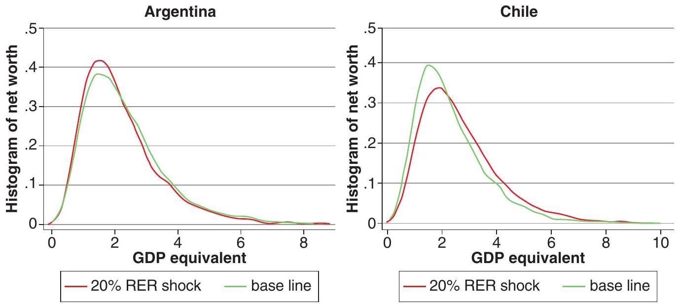
This so-called balance sheet approach has been shown to qualify quite dramatically the role played by explicit liabilities in determining the vulnerability or currency exposure of governments. For example, for many countries that issue debt in foreign currency, it is believed that a real exchange rate depreciation compromises fiscal sustainability because it increases the real value of debt. However, this statement should consider what other liabilities it has in domestic currency (say, wages), and how a real depreciation may increase its tax base. If the government collects a sizable fraction of its income, say, from export taxes, then its net worth may actually increase with a devaluation. An example is provided in Figure 17.3, by looking at the histogram of the NPV of government and its reaction to a real depreciation for Argentina and Chile.
Argentina, for example, shows an improvement in the net worth of the government as a result of a devaluation, in contrast with the results from the literature that focuses on explicit debt.
References
Alesina, A., Favero, C., & Giavazzi, F. (2019). Effects of austerity: Expenditure-and tax-based approaches. Journal of Economic Perspectives, 33(2), 141-62.
Alesina, A. & Giavazzi, F. (2013). Fiscal policy after the financial crisis. University of Chicago Press.
Ball, L., Furceri, D., Leigh, D., & Loungani, P. (2013). The distributional effects of fiscal austerity (tech. rep.) DESA Working Paper No. 129.
Barro, R. J. (1974). Are government bonds net wealth? Journal of Political Economy, 82(6), 1095-1117.
Barro, R. J. & Redlick, C. J. (2011). Macroeconomic effects from government purchases and taxes. The Quarterly Journal of Economics, 126(1), 51-102.
Blanchard, O. & Perotti, R. (2002). An empirical characterization of the dynamic effects of changes in government spending and taxes on output. The Quarterly Journal of Economics, 117(4), 1329-1368.
Ilzetzki, E., Mendoza, E. G., & Végh, C. A. (2013). How big (small?) are fiscal multipliers? Journal of Monetary Economics, 60(2), 239-254.
Levy-Yeyati, E. & Sturzenegger, F. (2007). A balance-sheet approach to fiscal sustainability. CID Working Paper Series.
Nakamura, E. & Steinsson, J. (2014). Fiscal stimulus in a monetary union: Evidence from U.S. regions. American Economic Review, 104(3), 753-92.
Ramey, V. A. (2009). Defense news shocks, 1939-2008: Estimates based on news sources. Unpublished paper, University of California, San Diego.
Ramey, V. A. & Shapiro, M. D. (1999). Costly capital reallocation and the effects of government spending. National Bureau of Economic Research.
Shoag, D. (2013). Using state pension shocks to estimate fiscal multipliers since the Great Recession. American Economic Review, 103(3), 121-24.
Is it really that easy? Let \(\bar{Y}\) be the steady state level of output, and, similarly, for \(C\) and \(G\). Now subtract \(\bar{Y}\) from both sides of the equation, and divide both sides by \(\bar{Y}\). Recognising that \(\bar{Y}=\bar{C}+\bar{G}\), this gives you \(\frac{Y_{t}-\bar{Y}}{\bar{Y}}=\frac{C_{t}-\bar{C}}{\bar{Y}}+\frac{G_{t}-\bar{G}}{\bar{Y}}\). Now multiply and divide the first term on the RHS by \(\bar{C}\), and the second term by \(\bar{G}\), and you will get the result.↩︎
Here’s how that one goes: note from the resource constraint that \(\hat{c}_{t}=\frac{1}{1-\gamma} \hat{y}_{t}-\frac{\gamma}{1-\gamma} \hat{g}_{t}\), and plug this into (17.29). Multiplying both sides by \((1-\gamma)\) yields \(\hat{y}_{t}=E_{t} \hat{y}_{t+1}-\gamma\left(E_{t} \hat{g}_{t+1}-\hat{g}_{t}\right)-\sigma(1-\gamma) r_{t}\). Define \(\Delta \hat{g}_{t+1}=\left(E_{t} \hat{g}_{t+1}-\hat{g}_{t}\right)\) and collect terms, and the result follows.↩︎
Recall that, for notational simplicity, we are leaving aside the terms in the discount rate and the productivity shock that shifts the natural rate of output, which is implicit within the log deviation term.↩︎