3 The neoclassical growth model







3.1 The Ramsey problem
We will solve the optimal savings problem underpinning the Neoclassical Growth Model, and in the process introduce the tools of dynamic optimisation we will use throughout the book. We will also encounter, for the first time, the most important equation in macroeconomics: the Euler equation.
\[ \frac{\dot{c}_{t}}{c_{t}}=\sigma\left[f^{\prime}\left(k_{t}\right)-\rho\right] \]
We have seen the lessons and shortcomings of the basic Solow model. One of its main assumptions, as you recall, was that the savings rate was constant. In fact, there was no optimisation involved in that model, and welfare statements are hard to make in that context. This is, however, a very rudimentary assumption for an able policy maker who is in possession of the tools of dynamic optimisation. Thus we tackle here the challenge of setting up an optimal program where savings is chosen to maximise intertemporal welfare.
As it turns out, British philosopher and mathematician Frank Ramsey, in one of the two seminal contributions he provided to economics before dying at the age of 26, solved this problem in 1928 (Ramsey (1928)).1 The trouble is, he was so ahead of his time that economists would only catch up in the 1960s, when David Cass and Tjalling Koopmans independently revived Ramsey’s contribution.2 (That is why this model is often referred to either as the Ramsey model or the Ramsey-Cass-Koopmans model.) It has since become ubiquitous and, under the grand moniker of Neoclassical Growth Model (NGM), it is the foremost example of the type of dynamic general equilibrium model upon which the entire edifice of modern macroeconomics is built.
To make the problem manageable, we will assume that there is one representative household, all of whose members are both consumer and producer, living in a closed economy (we will lift this assumption in the next chapter). There is one good and no government. Each consumer in the representative household lives forever, and population growth is \(n>0\) as before. All quantities in small-case letters are per capita. Finally, we will look at the problem as solved by a benevolent central planner who maximises the welfare of that representative household, and evaluates the utility of future consumption at a discounted rate.
At this point, it is worth stopping and thinking about the model’s assumptions. By now you are already used to outrageously unrealistic assumptions, but this may be a little too much. People
obviously do not live forever, they are not identical, and what’s this business of a benevolent central planner? Who are they? Why would they discount future consumption? Let us see why we use these shortcuts:
We will look at the central planner’s problem, as opposed to the decentralised equilibrium, because it is easier and gets us directly to an efficient allocation. We will show that, under certain conditions, it provides the same results as the decentralised equilibrium. This is due to the so-called welfare theorems, which you have seen when studying microeconomics, but which we should perhaps briefly restate here:
A competitive equilibrium is Pareto Optimal.
All Pareto Optimal allocations can be decentralised as a competitive equilibrium under some convexity assumptions. Convexity of production sets means that we cannot have increasing returns to scale. (If we do, we need to depart from competitive markets.)
There’s only one household? Certainly this is not very realistic, but it is okay if we think that typically people react similarly (not necessarily identically) to the parameters of the model. Specifically, do people respond similarly to an increase in the interest rate? If you think they do, then the assumption is okay.
Do all the people have the same utility function? Are they equal in all senses? Again, as above, not really. But, we believe they roughly respond similarly to basic tradeoffs. In addition, as shown by Caselli and Ventura (2000), one can incorporate a lot of sources of heterogeneity (namely, individuals can have different tastes, skills, initial wealth) and still end up with a representative household representation, as long as that heterogeneity has a certain structure. The assumption also means that we are, for the most part, ignoring distributional concerns, but that paper also shows that a wide range of distributional dynamics are compatible with that representation. (We will also raise some points about inequality as we go along.)
Do they live infinitely? Certainly not, but it does look like we have some intergenerational links. Barro (1974) suggests an individual who cares about the utility of their child: \(u\left(c_{t}\right)+\) \(\beta V\left[u\left(c_{\text {child }}\right)\right]\). If that is the case, substituting recursively gives an intertemporal utility of the sort we have posited. And people do think about the future.
Why do we discount future utility? To some extent it is a revealed preference argument: interest rates are positive and this only makes sense if people value more today’s consumption than tomorrow’s, which is what we refer to when we speak of discounting the future. On this you may also want to check Caplin and Leahy (2004), who argue that a utility such as that in (3.1) imposes a sort of tyranny of the present: past utility carries no weight, whereas future utility is discounted. But does this make sense from a planner’s point of view? Would this make sense from the perspective of tomorrow? In fact, Ramsey argued that it was unethical for a central planner to discount future utility.3
Having said that, let’s go solve the problem.
3.1.1 The consumer’s problem
The utility function is4
\[ \int_{0}^{\infty} u\left(c_{t}\right) e^{n t} e^{-\rho t} d t \tag{3.1}\]
where \(c_{t}\) denotes consumption per capita and \(\rho(>n)\) is the rate of time preference.5 Assume \(u^{\prime}\left(c_{t}\right)>0\), \(u^{\prime \prime}\left(c_{t}\right) \leq 0\), and Inada conditions are satisfied.
3.1.2 The resource constraint
The resource constraint of the economy is
\[ \dot{K}_{t}=Y_{t}-C_{t}=F\left(K_{t}, L_{t}\right)-C_{t}, \tag{3.2}\]
with all variables as defined in the previous chapter. (Notice that for simplicity we assume there is no depreciation.) In particular, \(F\left(K_{t}, L_{t}\right)\) is a neoclassical production function - hence neoclassical growth model. You can think of household production: household members own the capital and they work for themselves in producing output. Each member of the household inelastically supplies one unit of labour per unit of time.
This resource constraint is what makes the problem truly dynamic. The capital stock in the future depends on the choices that are made in the present. As such, the capital stock constitutes what we call the state variable in our problem: it describes the state of our dynamic system at any given point in time. The resource constraint is what we call the equation of motion: it characterises the evolution of the state variable over time. The other key variable, consumption, is what we call the control variable: it is the one variable that we can directly choose. Note that the control variable is jumpy: we can choose whatever (feasible) value for it at any given moment, so it can vary discontinuously. However, the state variable is sticky: we cannot change it discontinuously, but only in ways that are consistent with the equation of motion.
Given the assumption of constant returns to scale, we can express this constraint in per capita terms, which is more convenient. Dividing (3.2) through by \(L\) we get
\[ \frac{\dot{K}_{t}}{L_{t}}=F\left(k_{t}, 1\right)-c_{t}=f\left(k_{t}\right)-c_{t}, \tag{3.3}\]
where \(f(\).\() has the usual properties. Recall\)
\[ \frac{\dot{K}_{t}}{L_{t}}=\dot{k}_{t}+n k_{t} . \tag{3.4}\]
Combining the last two equations yields
\[ \dot{k}_{t}=f\left(k_{t}\right)-n k_{t}-c_{t}, \tag{3.5}\]
which we can think of as the relevant budget constraint. This is the final shape of the equation of motion of our dynamic problem, describing how the variable responsible for the dynamic nature of the problem - in this case the per capita capital stock \(k_{t}\) - evolves over time.
3.1.3 Solution to consumer’s problem
The household’s problem is to maximise (3.1) subject to (3.5) for given \(k_{0}\). If you look at our mathematical appendix, you will learn how to solve this, but it is instructive to walk through the steps here, as they have intuitive interpretations. You will need to set up the (current value) Hamiltonian for the problem, as follows:
\[ H=u\left(c_{t}\right) e^{n t}+\lambda_{t}\left[f\left(k_{t}\right)-n k_{t}-c_{t}\right] . \tag{3.6}\]
Recall that \(c\) is the control variable (jumpy), and \(k\) is the state variable (sticky), but the Hamiltonian brings to the forefront another variable: \(\lambda\), the co-state variable. It is the multiplier associated with the intertemporal budget constraint, analogously to the Lagrange multipliers of static optimisation.
Just like its Lagrange cousin, the co-state variable has an intuitive economic interpretation: it is the marginal value as of time \(t\) (i.e. the current value) of an additional unit of the state variable (capital, in this case). It is a (shadow) price, which is also jumpy.
First-order conditions (FOCs) are
\[ \frac{\partial H}{\partial c_{t}}=0 \Rightarrow u^{\prime}\left(c_{t}\right) e^{n t}-\lambda_{t}=0, \tag{3.7}\]
\[ \dot{\lambda}_{t}=-\frac{\partial H}{\partial k_{t}}+\rho \lambda_{t} \Rightarrow \dot{\lambda}_{t}=-\lambda_{t}\left[f^{\prime}\left(k_{t}\right)-n\right]+\rho \lambda_{t}, \tag{3.8}\]
\[ \lim _{t \rightarrow \infty}\left(k_{t} \lambda_{t} e^{-\rho t}\right)=0 . \tag{3.9}\]
What do these optimality conditions mean? First, (3.7) should be familiar from static optimisation: differentiate with respect to the control variable, and set that equal to zero. It makes sure that, at any given point in time, the consumer is making the optimal decision - otherwise, she could obviously do better… The other two are the ones that bring the dynamic aspects of the problem to the forefront. Equation (3.9) is known as the transversality condition (TVC). It means, intuitively, that the consumer wants to set the optimal path for consumption such that, in the “end of times” (at infinity, in this case), they are left with no capital. (As long as capital has a positive value as given by \(\lambda\), otherwise they don’t really care…) If that weren’t the case, I would be “dying” with valuable capital, which I could have used to consume a little more over my lifetime.
Equation (3.8) is the FOC with respect to the state variable, which essentially makes sure that at any given point in time the consumer is leaving the optimal amount of capital for the future. But how so? As it stands, it has been obtained mechanically. However, it is much nicer when we derive it purely from economic intuition. Note that we can rewrite it as follows:
\[ \frac{\dot{\lambda}_{t}}{\lambda_{t}}=\rho-\left(f^{\prime}\left(k_{t}\right)-n\right) \Rightarrow \rho+n=\frac{\dot{\lambda}_{t}}{\lambda_{t}}+f^{\prime}\left(k_{t}\right) . \tag{3.10}\]
This is nothing but an arbitrage equation for a typical asset price, where in this case the asset is the capital stock of the economy. Such arbitrage equations state that the opportunity cost of holding the asset ( \(\rho\) in this case), equals its rate of return, which comprises the dividend yield \(\left(f^{\prime}\left(k_{t}\right)-n\right)\) plus whatever capital gain you may get from holding the asset \(\left(\frac{\dot{\lambda}_{t}}{\lambda_{t}}\right)\). If the opportunity cost were higher (resp. lower), you would not be in an optimal position: you should hold less (resp. more) of the asset. We will come back to this intuition over and over again.
3.1.4 The balanced growth path and the Euler equation
We are ultimately interested in the dynamic behaviour of our control and state variables, \(c_{t}\) and \(k_{t}\). How can we turn our FOCs into a description of that behaviour (preferably one that we can represent graphically)? We start by taking (3.7) and differentiating both sides with respect to time:
\[ u^{\prime \prime}\left(c_{t}\right) \dot{c}_{t} e^{n t}+n u^{\prime}\left(c_{t}\right) e^{n t}=\dot{\lambda}_{t} . \tag{3.11}\]
Divide this by (3.7) and rearrange:
\[ \frac{u^{\prime \prime}\left(c_{t}\right) c_{t}}{u^{\prime}\left(c_{t}\right)} \frac{\dot{c}_{t}}{c_{t}}=\frac{\dot{\lambda}_{t}}{\lambda_{t}}-n . \tag{3.12}\]
Next, define
\[ \sigma \equiv-\frac{u^{\prime}\left(c_{t}\right)}{u^{\prime \prime}\left(c_{t}\right) c_{t}}>0 \tag{3.13}\]
as the elasticity of intertemporal substitution in consumption.6 Then, (3.12) becomes
\[ \frac{\dot{c}_{t}}{c_{t}}=-\sigma\left(\frac{\dot{\lambda}_{t}}{\lambda_{t}}-n\right) . \tag{3.14}\]
Finally, using (3.10) in (3.14) we obtain
\[ \frac{\dot{c}_{t}}{c_{t}}=\sigma\left[f^{\prime}\left(k_{t}\right)-\rho\right] . \tag{3.15}\]
This dynamic optimality condition is known as the Ramsey rule (or Keynes-Ramsey rule), and in a more general context it is referred to as the Euler equation. It may well be the most important equation in all of macroeconomics: it encapsulates the essence of the solution to any problem that trades off today versus tomorrow.7
But what does it mean intuitively? Think about it in these terms: if the consumer postpones the enjoyment of one unit of consumption to the next instant, it will be incorporated into the capital stock, and thus yield an extra \(f^{\prime}(\cdot)\). However, this will be worth less, by a factor of \(\rho\). They will only consume more in the next instant (i.e. \(\frac{\dot{c}_{t}}{c_{t}}>0\) ) if the former compensates for the latter, as mediated by their proclivity to switch consumption over time, which is captured by the elasticity of intertemporal substitution, \(\sigma\). Any dynamic problem we will see from now on involves some variation upon this general theme: the optimal growth rate trades off the rate of return of postponing consumption (i.e. investment) against the discount rate.
Mathematically speaking, equations (3.5) and (3.15) constitute a system of two differential equations in two unknowns. These plus the initial condition for capital and the TVC fully characterise the dynamics of the economy: once we have \(c_{t}\) and \(k_{t}\), we can easily solve for any remaining variables of interest.
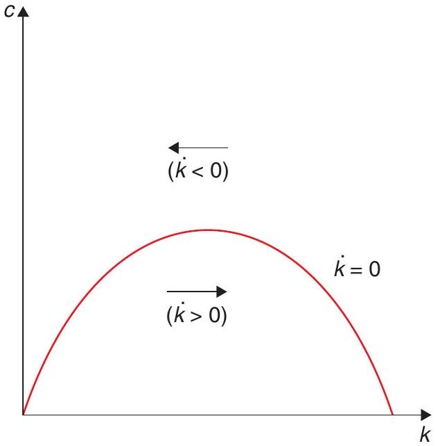
To make further progress, let us characterise the BGP of this economy. Setting (3.5) equal to zero yields
\[ c^{*}=f\left(k^{*}\right)-n k^{*}, \tag{3.16}\]
which obviously is a hump-shaped function in \(c, k\) space. The dynamics of capital can be understood with reference to this function (Figure 3.1): for any given level of capital, if consumption is higher (resp. lower) than the BGP level, this means that the capital stock will decrease (resp. increase).
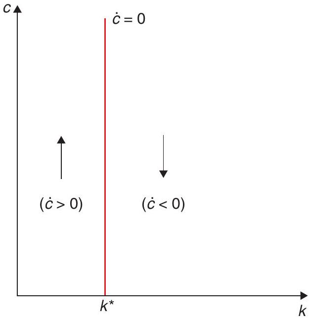
By contrast, setting (3.15) equal to zero yields
\[ f^{\prime}\left(k^{*}\right)=\rho . \tag{3.17}\]
This equation pins down the level of the capital stock on the BGP, and the dynamics of consumption can be seen in Figure 3.2: for any given level of consumption, if the capital stock is below (resp. above) its BGP level, then consumption is increasing (resp. decreasing). This is because the marginal product of capital will be relatively high (resp. low).
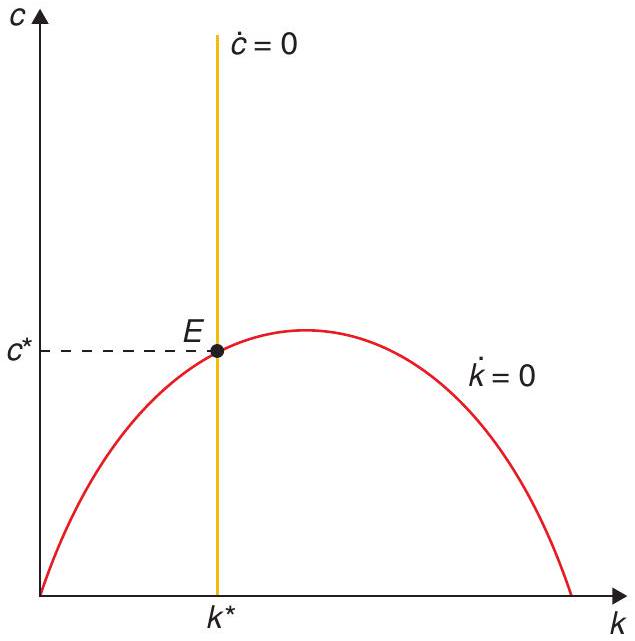
Expressions (3.16) and (3.17) together yield the values of consumption and the capital stock (both per-capita) in the BGP, as shown in Figure 3.3. This already lets us say something important about the behaviour of this economy. Let’s recall the concept of the golden rule, from our discussion of the
Solow model: the maximisation of per-capita consumption on the BGP. From (3.16) we see that this is tantamount to setting
\[ \frac{\partial c^{*}}{\partial k^{*}}=f^{\prime}\left(k_{G}^{*}\right)-n=0 \Rightarrow f^{\prime}\left(k_{G}^{*}\right)=n . \tag{3.18}\]
(Recall here we have assumed the depreciation rate is zero \((\delta=0)\).) If we compare this to (3.17), we see that the the optimal BGP level of capital per capita is lower than in the golden rule from the Solow model. (Recall the properties of the neoclassical production function, and that we assume \(\rho>n\).)
Because of this comparison, (3.17) is sometimes known as the modified golden rule. Why does optimality require that consumption be lower on the BGP than what would be prescribed by the Solow golden rule? Because future consumption is discounted, it is not optimal to save so much that BGP consumption is maximised - it is best to consume more along the transition to the BGP. Keep in mind that it is (3.17), not (3.18), that describes the optimal allocation. The kind of oversaving that is possible in the Solow model disappears once we consider optimal savings decisions.
Now, you may ask: is it the case then that this type of oversaving is not an issue in practice (or even just in theory)? Well, we will return to this issue in Chapter 8. For now, we can see how the question of dynamic efficiency relates to issues of inequality.
3.1.5 A digression on inequality: Is Piketty right?
It turns out that we can say something about inequality in the context of the NGM, even though the representative agent framework does not address it directly. Let’s start by noticing that, as in the Solow model, on the BGP output grows at the rate \(n\) of population growth (since capital and output per worker are constant). In addition, once we solve for the decentralised equilibrium, which we sketch in Section 2 below, we will see that in that equilibrium we have \(f^{\prime}(k)=r\), where \(r\) is the interest rate, or equivalently, the rate of return on capital.
This means that the condition for dynamic efficiency, which holds in the NGM, can be interpreted as the \(r>g\) condition made famous by Piketty (2014) in his influential Capital in the 21st Century. The condition \(r>g\) is what Piketty calls the “Fundamental Force for Divergence”: an interest rate that exceeds the growth rate of the economy. In short, he argues that, if \(r>g\) holds, then there will be a tendency for inequality to explode as the returns to capital accumulate faster than overall income grows. In Piketty’s words:
’This fundamental inequality (…) will play a crucial role in this book. In a sense, it sums up the overall logic of my conclusions. When the rate of return on capital significantly exceeds the growth rate of the economy (…), then it logically follows that inherited wealth grows faster than output and income.’ (pp. 25-26)
Does that mean that, were we to explicitly consider inequality in a context akin to the NGM we would predict it to explode along the BGP? Not so fast. First of all, when taking the model to the data, we could ask what \(k\) is. In particular, \(k\) can have a lot of human capital i.e. be the return to labour mostly, and this may help undo the result. In fact, it could even turn it upside down if human capital is most of the capital and is evenly distributed in the population. You may also want to see Acemoglu and Robinson (2015), who have a thorough discussion of this prediction. In particular, they argue that, in a model with workers and capitalists, modest amounts of social mobility - understood as a probability that some capitalists may become workers, and vice-versa - will counteract that force for divergence.
Yet the issue has been such a hot topic in the policy debate that two more comments on this issue are due.
First, let’s understand better the determinants of labour and income shares. Consider a typical Cobb-Douglas production function:
\[ Y=A L^{\alpha} K^{1-\alpha} . \tag{3.19}\]
With competitive factor markets, the FOC for profit maximisation would give:
\[ w=\alpha A L^{\alpha-1} K^{1-\alpha} . \tag{3.20}\]
Computing the labour share using the equilibrium wage gives:
\[ \frac{w L}{Y}=\frac{\alpha A L^{\alpha-1} K^{1-\alpha} L}{A L^{\alpha} K^{1-\alpha}}=\alpha, \tag{3.21}\]
which implies that for a Cobb-Douglas specification, labour and capital shares are constant. More generally, if the production function is
\[ Y=\left(\beta K^{\frac{\varepsilon-1}{\varepsilon}}+\alpha(A L)^{\frac{\varepsilon-1}{\varepsilon}}\right)^{\frac{\varepsilon}{\varepsilon-1}} \text { with } \varepsilon \in[0, \infty), \tag{3.22}\]
then \(\varepsilon\) is the (constant) elasticity of substitution between physical capital and labour. Note that when \(\varepsilon \rightarrow \infty\), the production function is linear ( \(K\) and \(L\) are perfect substitutes), and one can show that when \(\varepsilon \rightarrow 0\) the production function approaches the Leontief technology of fixed proportions, in which one factor cannot be substituted by the other at all.
From the FOC of profit maximisation we obtain:
\[ w=\left(\beta K^{\frac{\varepsilon-1}{\varepsilon}}+\alpha(A L)^{\frac{\varepsilon-1}{\varepsilon}}\right)^{\frac{1}{\varepsilon-1}} \alpha A(A L)^{-\frac{1}{\varepsilon}}, \tag{3.23}\]
the labour share is now:
\[ \frac{w L}{Y}=\frac{\alpha\left(\beta K^{\frac{\varepsilon-1}{\varepsilon}}+\alpha(A L)^{\frac{\varepsilon-1}{\varepsilon}}\right)^{\frac{1}{\varepsilon-1}} A^{\frac{\varepsilon-1}{\varepsilon}} L^{-\frac{1}{\varepsilon}} L}{\left(\beta K^{\frac{\varepsilon-1}{\varepsilon}}+\alpha(A L)^{\frac{\varepsilon-1}{\varepsilon}}\right)^{\frac{\varepsilon}{\varepsilon-1}}}=\alpha\left(\frac{A L}{Y}\right)^{\frac{\varepsilon-1}{\varepsilon}} . \tag{3.24}\]
Notice that as \(\frac{L}{Y} \longrightarrow 0\), several things can happen to the labour share, and what happens depends on \(A\) and \(\varepsilon\) :
\[ \text { If } \varepsilon>1 \Longrightarrow \alpha\left(\frac{A L}{Y}\right)^{\frac{\varepsilon-1}{\varepsilon}} \longrightarrow 0 \tag{3.25}\]
\[ \text { If } \varepsilon<1 \Longrightarrow \alpha\left(\frac{A L}{Y}\right)^{\frac{\varepsilon-1}{\varepsilon}} \text { increases. } \tag{3.26}\]
These two equations show that the elasticity of substitution is related to the concept of how essential a factor of production is. If the elasticity of substitution is less than one, the factor becomes more and more important with economic growth. If this factor is labour this may undo the Piketty result. This may be (and this is our last comment on the issue!) the reason why over the last centuries, while interest rates have been way above growth rates, inequality does not seem to have worsened. If anything, it seems to have moved in the opposite direction.
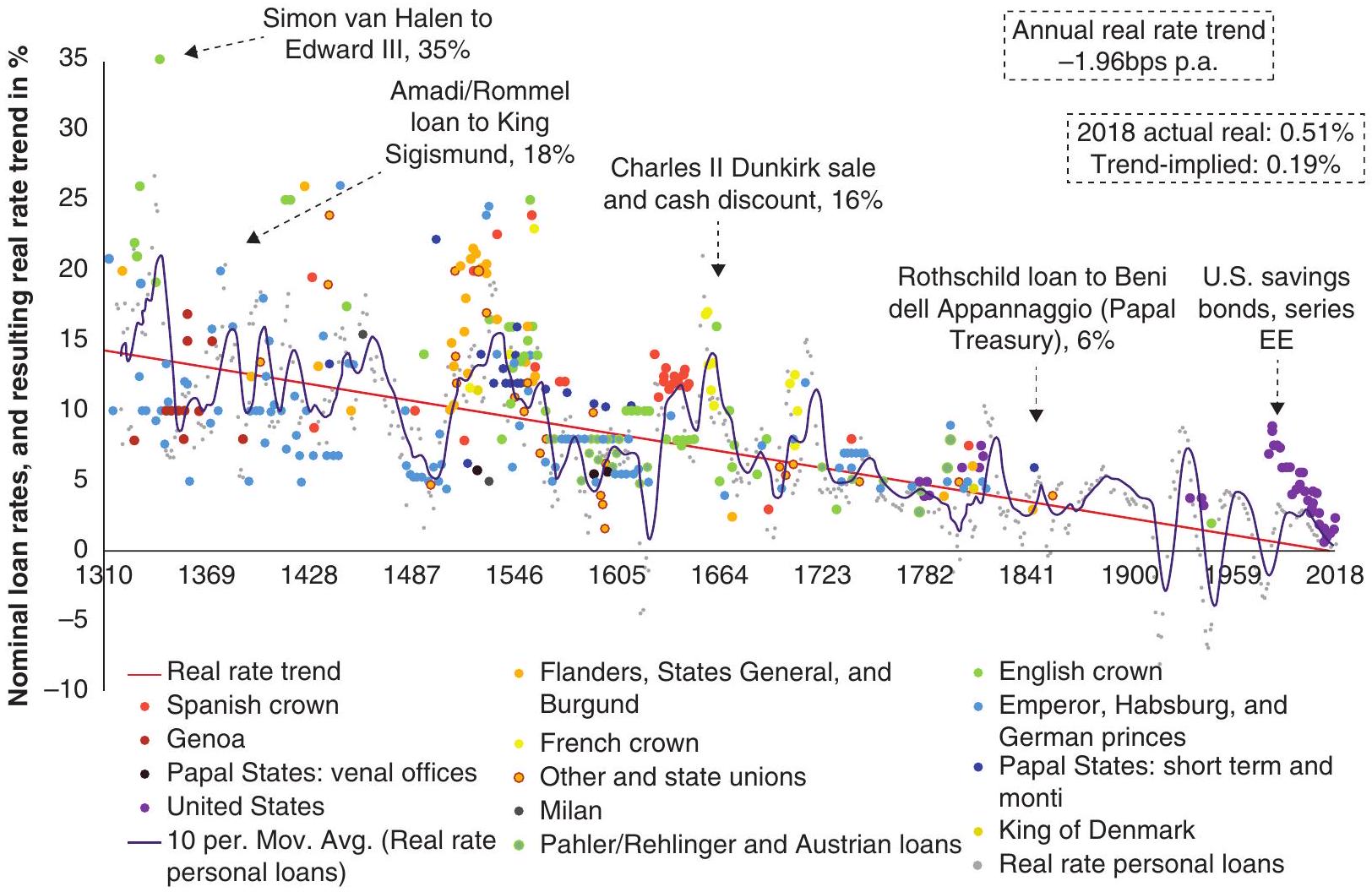
In Figure 3.4, Schmelzing (2019) looks at interest rates since the 1300s and shows that, while declining, they have consistently been above the growth rates of the economy at least until very recently. If those rates would have led to plutocracy, as Piketty fears, we would have seen it a long while ago. Yet the world seems to have moved in the opposite direction towards more democratic regimes.8
3.1.6 Transitional dynamics
How do we study the dynamics of this system? We will do so below graphically. But there are some shortcuts that allow you to understand the nature of the dynamic system, and particularly the relevant question of whether there is one, none, or multiple equilibria.
A dynamic system is a bunch of differential equations (difference equations if using discrete time). In the mathematical appendix, that you may want to refer to now, we argue that one way to approach this issue is to linearise the system around the steady state. For example, in our example here, Equations (3.5) and (3.15) are a system of two differential equations in two unknowns: \(c\) and \(k\). To linearise the system around the BGP or steady state we compute the derivatives relative to each variable as shown below:
\[ \left[\begin{array}{l} \dot{k}_{t} \\ \dot{c}_{t} \end{array}\right]=\Omega\left[\begin{array}{l} k_{t}-k^{*} \\ c_{t}-c^{*} \end{array}\right], \tag{3.27}\]
where
\[ \Omega=\left[\left.\left.\begin{array}{ll} \frac{\partial \dot{k}}{\partial k} \\ \frac{\partial \dot{c}}{\partial k} \end{array}\right|_{S S} \frac{\frac{\partial \dot{k}}{\partial c}}{\frac{\partial \dot{c}}{\partial c}}\right|_{S S}\right] \tag{3.28}\]
and
\[ \left.\frac{\partial \dot{k}}{\partial k}\right|_{S S}=f^{\prime}\left(k^{*}\right)-n=\rho-n \tag{3.29}\]
\[ \left.\frac{\partial \dot{k}}{\partial c}\right|_{S S}=-1 \tag{3.30}\]
\[ \left.\frac{\partial \dot{c}}{\partial k}\right|_{S S}=\sigma c^{*} f^{\prime \prime}\left(k^{*}\right) \tag{3.31}\]
\[ \left.\frac{\partial \dot{c}}{\partial c}\right|_{S S}=0 . \tag{3.32}\]
These computations allow us to define a matrix with the coefficients of the response of each variable to those in the system, at the steady state. In this case, this matrix is
\[ \Omega=\left[\begin{array}{cc} \rho-n & -1 \\ \sigma c^{*} f^{\prime \prime}\left(k^{*}\right) & 0 \end{array}\right] . \tag{3.33}\]
In the mathematical appendix we provide some tools to understand the importance of this matrix of coefficients. In particular, this matrix has two associated eigenvalues, call them \(\lambda_{1}\) and \(\lambda_{2}\) (not to be confused with the marginal utility of consumption). The important thing to remember from the appendix is that the dynamic equations for the variables will be of the form \(A e^{\lambda_{1}}+B e^{\lambda_{2}}\). Thus, the nature of these eigenvalues turns out to be critical for understanding the dynamic properties of the system. If they are negative their effect dilutes over time (this configuration is called a sink, as variables converge to their steady state). If positive, the variable blows up (we call these systems a source, where variables drift away from the steady state). If one is positive and the other is negative the system typically blows up, except if the coefficient of the positive eigenvalue is zero (we call these saddle-path systems).
You may think that what you want is a sink, a system that converges to an equilibrium. While this may be the natural approach in sciences such as physics, this reasoning would not be correct in the realm of economics. Imagine you have one state variable (not jumpy) and a control variable (jumpy), as in this system. In the system we are analysing here \(k\) is a state variable that moves slowly over time and \(c\)
is the control variable that can jump. So, if you have a sink, you would find that any \(c\) would take you to the equilibrium. So rather than having a unique stable equilibrium you would have infinite alternative equilibria! Only if the two variables are state variables do you want a sink. In this case the equilibrium is unique because the state variables are uniquely determined at the start of the program.
In our case, to pin down a unique equilibria we would need a saddle-path configuration. Why? Because for this configuration there is only one value of the control variable that makes the coefficient of the explosive eigenvalue equal to zero. This feature is what allows to pin the unique converging equilibria. In the figures below this will become very clear.
What happens if all variables are control variables? Then you need the system to be a source, so that the control variables have only one possible value that attains sustainability. We will find many systems like this throughout the book.
In short, there is a rule that you may want to keep in mind. You need as many positive eigenvalues as jumpy or forward-looking variables you have in your system. If these two numbers match you have uniqueness!9
Before proceeding, one last rule you may want to remember. The determinant of the matrix is the product of the eigenvalues, and the trace is equal to the sum. This is useful, because, for example, in our two-equation model, if the determinant is negative, this means that the eigenvalues have different sign, indicating a saddle path. In fact, in our specific case,
- \(\operatorname{Det}(\Omega)=\sigma c^{*} f^{\prime \prime}\left(k^{*}\right)<0\).
If \(\operatorname{Det}(\Omega)\) is the product of the eigenvalues of the matrix \(\Omega\) and their product is negative, then we know that the eigenvalues must have the opposite sign. Hence, we conclude one eigenvalue is positive, while the other is negative.
Recall that \(k\) is a slow-moving, or sticky, variable, while \(c\) can jump. Hence, since we have the same number of negative eigenvalues as of sticky variables, we conclude the system is saddle-path stable, and the convergence to the equilibrium unique. You can see this in a much less abstract way in the the phase diagram in Figure 3.5.
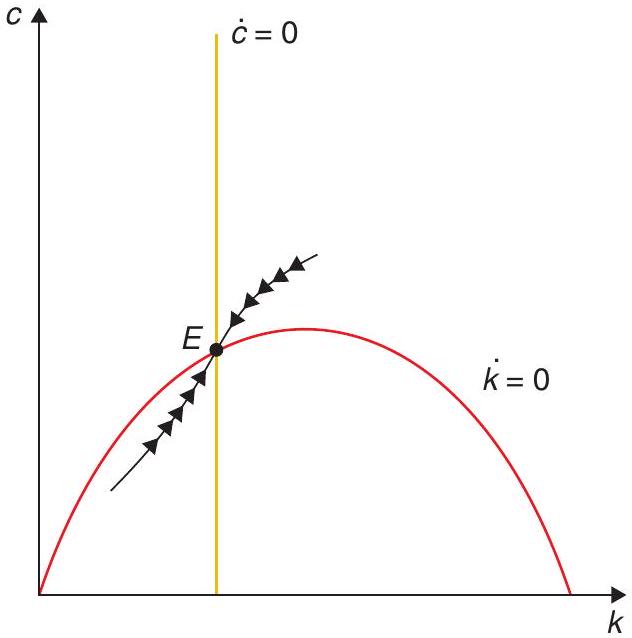
Notice that since \(c\) can jump, from any initial condition for \(k(0)\), the system moves vertically ( \(c\) moves up or down) to hit the saddle path and converge to the BGP along the saddle path. Any other trajectory is divergent. Alternative trajectories appear in Figure 3.6.
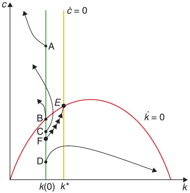
The problem is that these alternative trajectories either eventually imply a jump in the price of capital, which is inconsistent with rationality, or imply above-optimal levels of the capital stock. In either case this violates the transversality condition. In short, the first two dynamic equations provide the dynamics at any point in the \((c, k)\) space, but only the TVC allows us to choose a single path that we will use to describe our equilibrium dynamics.10
3.1.7 The effects of shocks
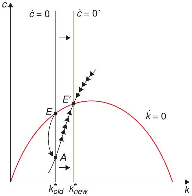
Consider the effects of the following shock. At time 0 and unexpectedly, the discount rate falls forever (people become less impatient). From the relevant \(\dot{k}=0\) and \(\dot{c}=0\) schedules, we see that the former does not move ( \(\rho\) does not enter) but the latter does. Hence, the new BGP will have a higher capital stock. It will also have higher consumption, since capital and output are higher. Figure 3.7 shows the old BGP, the new BGP, and the path to get from one to the other. On impact, consumption falls (from point \(E\) to point \(A\) ). Thereafter, both \(c\) and \(k\) rise together until reaching point \(E^{\prime}\).
Similar exercises can be carried out for other permanent and unanticipated shocks.
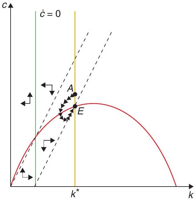
Consider, for example, an increase in the discount rate (Figure 3.8). (The increase is transitory, and that is anticipated by the planner.) The point we want to make is that there can be no anticipated jump in the control variables throughout the optimal path as this would allow for infinite capital gains. This is why the trajectory has to put you on the new saddle path when the discount rate goes back to normal.
3.2 The equivalence with the decentralised equilibrium
We will show that the solution to the central planner’s problem is exactly the same as the solution to a decentralised equilibrium.
Now we will sketch the solution to the problem of finding the equilibrium in an economy that is identical to the one we have been studying, but without a central planner. We now have households
and firms (owned by households) who independently make their decisions in a perfectly competitive environment. We will only sketch this solution.
The utility function to be maximised by each household is
\[ \int_{0}^{\infty} u\left(c_{t}\right) e^{n t} e^{-\rho t} d t \tag{3.34}\]
where \(c_{t}\) is consumption and \(\rho(>n)\) is the rate of time preference.
The consumer’s budget constraint can be written as
\[ c_{t} L_{t}+\dot{A}=w_{t} L_{t}+r A_{t}, \tag{3.35}\]
where \(L_{t}\) is population, \(A_{t}\) is the stock of assets, \(\dot{A}\) is the increase in assets, \(w_{t}\) is the wage per unit of labour (in this case per worker), and \(r\) is the return on assets. What are these assets? The households own the capital stock that they then rent out to firms in exchange for a payment of \(r\); they can also borrow and lend money to each other, and we denote their total debt by \(B_{t}\). In other words, we can define
\[ A_{t}=K_{t}-B_{t} . \tag{3.36}\]
You should be able to go from (3.35) to the budget constraint in per worker terms:
\[ c_{t}+\frac{d a_{t}}{d t}+n a_{t}=w_{t}+r a_{t} . \tag{3.37}\]
Households supply factors of production, and firms maximise profits. Thus, at each moment, you should be able to show that equilibrium in factor markets involves
\[ r_{t}=f^{\prime}\left(k_{t}\right), \tag{3.38}\]
\[ w_{t}=f\left(k_{t}\right)-f^{\prime}\left(k_{t}\right) k_{t} . \tag{3.39}\]
In this model, we must impose what we call a no-Ponzi-game (NPG) condition.11 What does that mean? That means that households cannot pursue the easy path of getting arbitrarily rich by borrowing money and borrowing even more to pay for the interest owed on previously contracted debt. If possible that would be the optimal solution, and a rather trivial one at that. The idea is that the market will not allow these Ponzi schemes, so we impose this as a constraint on household behaviour.
\[ \lim _{t \rightarrow \infty} a_{t} e^{-(r-n) t} \geq 0 \tag{3.40}\]
You will have noticed that this NPG looks a bit similar to the TVC we have seen in the context of the planner’s problem, so it is easy to mix them up. Yet, they are different! The NPG is a constraint on optimisation - it wasn’t needed in the planner’s problem because there was no one in that closed economy from whom to borrow. In contrast, the TVC is an optimality condition - that is to say, something that is chosen in order to achieve optimality. They are related, in that both pertain to what happens in the limit, as \(t \rightarrow \infty\). We will see how they help connect the decentralised equilibrium with the planner’s problem.
3.2.1 Integrating the budget constraint
The budget constraint in (3.37) holds at every instant \(t\). It is interesting to figure out what it implies for the entire path to be chosen by households. To do this, we need to integrate that budget constraint. In future chapters we will assume that you know how to do this integration, and you can consult the mathematical appendix for that. But the first time we will go over all the steps.
So let’s start again with the budget constraint for an individual family:
\[ \dot{a}_{t}-(r-n) a_{t}=w_{t}-c_{t} . \tag{3.41}\]
This is a first-order differential equation which (as you can see in the Mathematical Appendix) can be solved using integrating factors. To see how that works, multiply both sides of this equation by \(e^{-(r-n) t}\) :
\[ \dot{a}_{t} e^{-(r-n) t}+(n-r) a_{t} e^{-(r-n) t}=\left(w_{t}-c_{t}\right) e^{-(r-n) t} . \tag{3.42}\]
The left-hand side is clearly the derivative of \(a_{t} e^{(n-r) t}\) with respect to time, so we can integrate both sides between 0 and \(t\) :
\[ a_{t} e^{-(r-n) t}-a_{0}=\int_{0}^{t}\left(w_{s}-c_{s}\right) e^{-(r-n) s} d s . \tag{3.43}\]
Taking the \(\lim t \longrightarrow \infty\) (and using the no-Ponzi condition) yields:
\[ 0=\int_{0}^{\infty}\left(w_{s}-c_{s}\right) e^{-(r-n) s} d s+a_{0} \tag{3.44}\]
which can be written as a standard intertemporal budget constraint:
\[ \int_{0}^{\infty} w_{s} e^{-(r-n) s} d s+a_{0}=\int_{0}^{\infty} c_{s} e^{-(r-n) s} d s \tag{3.45}\]
This is quite natural and intuitive: all of what is consumed must be financed out of initial assets or wages (since we assume that Ponzi schemes are not possible).
3.2.2 Back to our problem
Now we can go back to solve the consumer’s problem
\[ \operatorname{Max} \int_{0}^{\infty} u\left(c_{t}\right) e^{n t} e^{-\rho t} d t \tag{3.46}\]
s.t.
\[ c_{t}+\dot{a}+(n-r) a_{t}=w_{t} . \tag{3.47}\]
The Hamiltonian now looks like this
\[ H=u\left(c_{t}\right) e^{n t}+\lambda_{t}\left[w_{t}-c_{t}-(n-r) a_{t}\right] . \tag{3.48}\]
From this you can obtain the FOCs and, following the same procedure from the previous case, you should be able to get to
\[ -c_{t} \frac{u^{\prime \prime}\left(c_{t}\right)}{u^{\prime}\left(c_{t}\right)} \frac{\dot{c}_{t}}{c_{t}}=(r-\rho) . \tag{3.49}\]
How does that compare to (3.15), the Euler equation, which is one of our dynamic equations in the central planner’s solution? We leave that to you.
You will also notice that, from the equivalent FOCs (3.7) and (3.8), we have
\[ \frac{\dot{u}^{\prime}}{u^{\prime}}=(\rho-r), \tag{3.50}\]
or
\[ u^{\prime}\left(c_{t}\right)=e^{(\rho-r) t} . \tag{3.51}\]
Using this in the equivalent of (3.7) yields:
\[ e^{(n-r) t}=\lambda_{t} e^{-\rho t} . \tag{3.52}\]
This means that the NPG becomes:
\[ \lim _{t \rightarrow \infty} a_{t} \lambda_{t} e^{-\rho t}=\lim _{t \rightarrow \infty} a_{t} e^{-(r-n) t} . \tag{3.53}\]
You can show that this is exactly the same as the TVC for the central planner’s problem. (Think about it: since all individuals are identical, what is the equilibrium level of \(b_{t}\) ? If an individual wants to borrow, would anyone else want to lend?)
Finally, with the same reasoning on the equilibrium level of \(b_{t}\), you can show that the resource constraint also matches the dynamic equation for capital, (3.5), which was the relevant resource constraint for the central planner’s problem.
3.3 Do we have growth after all?
Not really.
Having seen the workings of the Ramsey model, we can see that on the BGP, just as in the Solow model, there is no growth in per capita variables: \(k\) is constant at \(k^{*}\) such that \(f^{\prime}\left(k^{*}\right)=\rho\), and \(y\) is constant at \(f\left(k^{*}\right)\). (It is easy to show that once again we can obtain growth if we introduce exogenous technological progress.)
3.4 What have we learned?
We are still left with a growth model without long-run growth: it was not the exogeneity of the savings rate that generated the unsatisfactory features of the Solow model when it comes to explaining longrun growth. We will have to keep looking by moving away from diminishing returns or by modelling technological progress.
On the other hand, our exploration of the Ramsey model has left us with a microfounded framework that is the foundation of a lot of modern macroeconomics. This is true not only of our further explorations that will lead us into endogenous growth, but eventually also when we move to the realm of short term fluctuations. At any rate, the NGM is a dynamic general equilibrium framework that we will use over and over again.
Even in this basic application some key results have emerged. First, we have the Euler equation that encapsulates how consumers make optimal choices between today and tomorrow. If the marginal benefit of reducing consumption - namely, the rate of return on the extra capital you accumulate -
is greater than the consumer’s impatience - the discount rate - then it makes sense to postpone consumption. This crucial piece of intuition will appear again and again as we go along in the book, and is perhaps the key result in modern macroeconomics. Second, in this context there is no dynamic inefficiency, as forward-looking consumers would never choose to oversave in an inefficient way.
Most importantly, now we are in possession of a powerful toolkit for dynamic analysis, and we will make sure to put it to use from now on.
it cannot continue. When that happens the price of capital increases, and consumers would have arbitraged that jump away, so that that path would have not occurred in the first place.
References
Acemoglu, D. & Robinson, J. A. (2015). The rise and decline of general laws of capitalism. Journal of Economic Perspectives, 29(1), 3-28.
Barro, R. J. (1974). Are government bonds net wealth? Journal of Political Economy, 82(6), 1095-1117.
Caplin, A. & Leahy, J. (2004). The social discount rate. Journal of Political Economy, 112(6), 1257-1268.
Caselli, F. & Ventura, J. (2000). A representative consumer theory of distribution. American Economic Review, 90(4), 909-926.
Cass, D. (1965). Optimum growth in an aggregative model of capital accumulation. The Review of Economic Studies, 32(3), 233-240.
Koopmans, T. C. et al. (1963). On the concept of optimal economic growth (tech. rep.) Cowles Foundation for Research in Economics, Yale University.
Piketty, T. (2014). Capital in the twenty-first century. Harvard University Press.
Ramsey, F. P. (1927). A contribution to the theory of taxation. The Economic Journal, 37(145), 47-61.
Ramsey, F. P. (1928). A mathematical theory of saving. The Economic Journal, 38(152), 543-559.
Schmelzing, P. (2019). Eight centuries of global real rates, r-g, and the ’suprasecular’ decline, 1311-2018, Available at SSRN: https://ssrn.com/abstract=3485734 or http://dx.doi.org/10.2139/ssrn.3485734.
The other one was to the theory of optimal taxation (Ramsey 1927).↩︎
See Cass (1965) and Koopmans et al. (1963).↩︎
Another interesting set of questions refer to population policies: say you impose a policy to reduce population growth. How does that play into the utility function? How do you count people that have not been and will not be born? Should a central planner count those people?↩︎
We are departing from standard mathematical convention, by using subscripts instead of parentheses to denote time, even though we are modelling time as continuous and not discrete. We think it pays off to be unconventional, in terms of making notation look less cluttered, but we apologise to the purists in the audience nonetheless!↩︎
Note that we must assume that \(\rho>n\), or the problem will not be well-defined. Why? Because if \(\rho<n\), the representative household gets more total utility out of a given level of consumption per capita in the future as there will be more “capitas” then. If the discount factor does not compensate for that, it would make sense to always postpone consumption! And why do we have \(e^{n t}\) in the utility function in the first place? Because we are incorporating the utility of all the individuals who are alive at time \(t\) - the more, the merrier!↩︎
Recall that the elasticity of a variable \(x\) with respect to another variable \(y\) is defined as \(\frac{\frac{d x}{d y}}{\frac{x}{y}}\). As such, \(\frac{1}{\sigma}\) is the elasticity of the marginal utility of consumption with respect to consumption - it measures how sensitive the marginal utility is to increases in consumption. Now, think about it: the more sensitive it is, the more I will want to smooth consumption over time, and this means I will be less likely to substitute consumption over time. That is why the inverse of that captures the intertemporal elasticity of substitution: the greater \(\sigma\) is, the more I am willing to substitute consumption over time.↩︎
This is the continuous-time analogue of the standard optimality condition that you may have encountered in microeconomics: the marginal rate of substitution (between consumption at two adjacent points in time) must be equal to the marginal rate of transformation.↩︎
At any rate, it may also be argued that maybe we haven’t seen plutocracies because Piketty was right. After all, the French and U.S. revolutions may be explained by previous increases in inequality.↩︎
It works the same for a system of difference equation in discrete time, except that the cutoff is with eigenvalues being larger or smaller than one.↩︎
To rule out the path that leads to the capital stock of when the \(\dot{k}=0\) locus crosses the horizontal axis to the right of the golden rule, notice that \(\lambda\) from (3.8) grows at the rate \(\rho+n-f^{\prime}(k)\) so that \(\lambda e^{-\rho t}\) grows at rate \(n-f^{\prime}(k)\), but to the right of the golden rule \(n>f^{\prime}(k)\), so that the term increases. Given that the capital stock is eventually fixed we conclude that the transversality condition cannot hold. The paths that lead to high consumption and a zero capital stock imply a collapse of consumption to zero when the path reaches the vertical axis. This trajectory is not feasible because at some point↩︎
Or should it now be the no-Madoff-game condition?↩︎