18  Fiscal policy II: The long-run determinants of fiscal policy

In our previous chapter we learned that it may be quite misleading to think about fiscal policy without thinking about the budget constraint. Our overarching question was whether fiscal policy can actually affect aggregate demand, and the central message was that the existence of budget constraints limits substantially what fiscal policy can do in that domain. In particular, all fiscal policy interventions will have to be eventually paid for, and rational individuals will understand that and adjust their consumption in ways that might undo the effects of those interventions - completely or partially, depending on the nature of the latter. Fiscal policy is more constrained than our old IS-LM world had led us to believe.

This relatively muted effect on aggregate demand, led to skepticism with respect to the prospects of government spending as a tool for macroeconomic stabilisation, with monetary policy taking over as the go-to aggregate demand management tool. In fact, over the years, Central Bankers have taken a much more prominent role in managing stabilisation policies than fiscal policy. (The very low interest rates of recent times changed more than a few minds on this point, particularly because of the zerorate lower bound issue. We will turn to that in due course.)

In any event, this leads us to think of fiscal policy as it relates to the needs for public good provision, the second angle we highlighted at the start of the last chapter. We can think of this as a long-run view: that of setting up a system aimed at providing these public goods (though keeping in mind that some of these may depend on the cycle, such as unemployment insurance). With this view in mind, how should the level of government spending and taxes move over time? How stable should they be?

In order to think that optimal long-run fiscal policy we will initially consider a government that faces an exogenous stream of government expenditures (public goods and entitlements, which may be shocked by natural disasters, wars, pandemics, etc.) How should it finance them? What should the path of taxes and borrowing be?

As it turns out, with non-distortionary taxation, long-lived individuals, and perfect capital markets, we know that this choice is inconsequential: it’s the world of Ricardian equivalence! But assume now that taxes are in fact distortionary, so that a high tax rate is costly - for instance, because it reduces incentives to work and/or to invest. What should the government do? After analysing this problem,

we will discuss the decision of how government spending itself may react to shocks. If income falls, should government expenditure remain the same?

We then go over the question of whether fiscal policy, in practice, behaves in the way that theory would prescribe. The answer is that, of course, there are significant departures, because policy makers are often not behaving in the way our simple theory suggests - in particular, they are not benevolent planners, but rather part of an often messy political process. We need to get into the political economy of fiscal policy to think through these issues.

Finally, we briefly address the issue of what type of taxes should be raised to finance government expenditure, in particular whether it makes sense to finance expenditures with taxes on labor or taxes on capital. While this is a topic that overlaps with issues discussed in the field of public finance, it delivers a remarkable result with implications for capital accumulation, and therefore for the macroeconomics discussion.

But let’s start at the beginning by looking at the optimal path for aggregate taxes.

18.1 Tax smoothing

We establish the tax smoothing principle, that suggests a countercyclical pattern for fiscal policy: one should run deficits when spending needs are higher than normal, and surpluses when they are below normal. By the same token, temporary expenditures should be financed by deficits.

Let \(g_{t}\) and \(\tau_{t}\) denote the government’s real purchases and tax revenues at time \(t\), and \(d_{0}\) is the initial real debt outstanding. The budget deficit is

\[ \dot{d}_{t}=\left(g_{t}-\tau_{t}\right)+r d_{t}, \tag{18.1}\]

where \(r\) is the real interest rate.

The government is also constrained by the standard solvency condition:

\[ \lim _{T \rightarrow \infty}\left(d_{T} e^{-r T}\right) \leq 0, \tag{18.2}\]

In the limit the present value of its debt cannot be positive.

18.1.1 The government objective function

The government wants to minimise tax distortions:

\[ L=\int_{0}^{\infty} y_{t} \ell\left(\frac{\tau_{t}}{y_{t}}\right) e^{-r t} d t \tag{18.3}\]

where \(\ell(0)=0, \ell(.)^{\prime}>0\) and \(\ell^{\prime \prime}()>\).0 . This function is a shorthand to capture the fact that taxes usually distort investment and labour-supply decisions, such that the economy (the private sector) suffers a loss, which is higher the higher is the ratio of tax revenues to income. Notice that we can think of the ratio \(\frac{\tau_{t}}{y_{t}}\) as the tax rate. The loss function is also convex: the cost increases at an increasing rate as the tax rate \(\frac{\tau_{t}}{y_{t}}\) rises. Notice also that these are pecuniary losses, which the government discounts at the rate of interest.

18.1.2 Solving the government’s problem

Assume that the government controls tax revenue \(\tau_{t}\) (which becomes the control variable) while government spending \(g_{t}\) is given. The Hamiltonian for the problem is

\[ H=y_{t} \ell\left(\frac{\tau_{t}}{y_{t}}\right)+\lambda_{t}\left(g_{t}-\tau_{t}+r d_{t}\right), \tag{18.4}\]

where \(\operatorname{debt} d_{t}\) is the state variable and \(\lambda_{t}\) the costate. The FOCs are

\[ \ell^{\prime}\left(\frac{\tau_{t}}{y_{t}}\right)=\lambda_{t}, \tag{18.5}\]

\[ \dot{\lambda}_{t}=\lambda_{t}(r-r)=0, \tag{18.6}\]

\[ \lim _{T \rightarrow \infty}\left(\lambda_{T} d_{T} e^{-r T}\right)=0 . \tag{18.7}\]

18.1.3 The time profile of tax distortions

The combination of (18.5) and (18.6) implies that tax revenue as a share of output should be constant along a perfect foresight path:

\[ \ell^{\prime}\left(\frac{\tau_{t}}{y_{t}}\right)=\lambda \text { for all } t \geq 0 \text {. } \tag{18.8}\]

We call this tax smoothing. The intuition is the same as in consumption smoothing. With the rate of interest equal to the rate at which loss is discounted, there is no incentive to have losses be higher in one moment than in another. The intuition is that, because the marginal distortion cost per unit of revenue raised is increasing in the tax rate (the ratio \(\frac{\tau_{t}}{y_{t}}\) ), a smooth tax rate minimises distortion costs.

Denote the implicit tax rate by

\[ \phi_{t}=\frac{\tau_{t}}{y_{t}} . \tag{18.9}\]

Expression (18.8) says that along a perfect foresight path, the tax rate should be constant:

\[ \phi_{t}=\frac{\tau_{t}}{y_{t}}=\phi \text { for all } t . \tag{18.10}\]

This is known as the “tax smoothing” principle, and is the key result of the paper by Barro (1979).¹

Notice also that, if \(\lambda\) is constant and non-zero, the TVC (18.7) implies that

\[ \lim _{T \rightarrow \infty}\left(d_{T} e^{-r T}\right)=0 . \tag{18.11}\]

That is, the solvency condition will hold with equality. Since the shadow value of debt is always positive, the government will choose to leave behind as much debt as possible (in present value) - that is to say, zero.

18.1.4 The level of tax distortions

Solving (18.1) forward starting from some time 0 yields

\[ d_{T} e^{-r T}=d_{0}+\int_{0}^{T}\left(g_{t}-\tau_{t}\right) e^{-r t} d t \tag{18.12}\]

Next, apply to this last equation the transversality/solvency condition (18.11) to get

\[ \lim _{T \rightarrow \infty}\left(d_{T} e^{-r T}\right)=d_{0}+\int_{0}^{\infty}\left(g_{t}-\tau_{t}\right) e^{-r t} d t=0 \tag{18.13}\]

Rearranging, this becomes

\[ \int_{0}^{\infty} \tau_{t} e^{-r t} d t=d_{0}+\int_{0}^{\infty} g_{t} e^{-r t} d t \tag{18.14}\]

But, given (18.10), this can be rewritten as

\[ \phi \int_{0}^{\infty} y_{t} e^{-r t} d t=d_{0}+\int_{0}^{\infty} g_{t} e^{-r t} d t \tag{18.15}\]

or

\[ \phi=\frac{d_{0}+\int_{0}^{\infty} g_{t} e^{-r t} d t}{\int_{0}^{\infty} y_{t} e^{-r t} d t} \tag{18.16}\]

That is to say, the optimal flat tax rate equals the ratio of the present value of the revenue the government must raise to the present value of output.

18.1.5 The steady state

Imagine that initially both output and expenditures are expected to remain constant, at levels \(g_{t}=g^{L}\) and \(y_{t}=y\). Then, (18.16) implies

\[ \tau=\phi y=r d_{0}+g^{L}, \tag{18.17}\]

so that the chosen tax revenue is equal to the permanent expenditures of government. Using this result in budget constraint (18.1) we have

\[ \dot{d}_{t}=r d_{t}+g^{L}-\tau_{t}=r d_{t}+g^{L}-r d_{0}-g^{L}=r\left(d_{t}-d_{0}\right) . \tag{18.18}\]

Evaluating this expression at time 0 we obtain

\[ \dot{d}_{0}=r\left(d_{0}-d_{0}\right)=0 . \tag{18.19}\]

Hence, the stock of debt is constant as well.

18.1.6 Changes in government expenditures

Suppose now that at time 0 there is an unanticipated and permanent increase in spending from \(g^{L}\) to \(g^{H}\). From (18.17) it follows that tax revenue adjusts instantaneously to its new (and higher) value:

\[ \tau^{\prime}=\phi^{\prime} y=r d_{0}+g^{H}, \quad t \geq 0 . \tag{18.20}\]

The adjustment takes place via an increase in the tax rate \(\phi\), to a higher level \(\phi^{\prime}\). Since revenues increases one-to-one with government spending, fiscal deficit does not change. Hence, an unanticipated and permanent increase in spending has no impact on the deficit nor on government debt.

How about temporary shocks? Suppose that the economy is in the initial steady-state described above, with revenue given by (18.17). At time 0, there is an unanticipated and temporary increase in spending:

\[ g_{t}= \begin{cases}g^{H}, & 0 \leq t<T \\ g^{L}, & t \geq T,\end{cases} \tag{18.21}\]

for some \(T>0\).

First compute the revenue path. Expression (18.16) becomes

\[ \phi=\frac{r d_{0}+r \int_{0}^{\infty} g_{t} e^{-r t} d t}{y} . \tag{18.22}\]

Combining (18.21) and (18.22) we have that revenue rises immediately to the level given by:

\[ \tau^{\prime \prime}=\phi^{\prime \prime} y=r d_{0}+g^{H}\left(1-e^{-r T}\right)+g^{L} e^{-r T}, \quad t \geq 0 . \tag{18.23}\]

where \(\phi^{\prime \prime}>\phi\) is now the new and constant tax rate.

Note that, quite naturally, the increase in the tax rate is lower under the temporary increase in spending than under the permanent increase:

\[ \phi^{\prime}-\phi^{\prime \prime}=\frac{\left(g^{H}-g^{L}\right) e^{-r T}}{y}>0 . \tag{18.24}\]

Next, compute the path for the fiscal deficit. Plugging (18.23) into (18.1) we have

\[ \dot{d}_{t}=r\left(d_{t}-d_{0}\right)+\left(g^{H}-g^{L}\right) e^{-r T}, \quad 0 \leq t<T . \tag{18.25}\]

Notice that at time \(t=0\) this implies

\[ \dot{d}_{0}=\left(g^{H}-g^{L}\right) e^{-r T}>0 . \tag{18.26}\]

There is a fiscal deficit \(\left(\dot{d}_{0}>0\right)\) from the start. From (18.25), this means that \(d_{t}>d_{0}\) for all times between 0 and \(T\). The fiscal deficit worsens over time and then jumps back to zero at time \(T\). Figure 18.1 shows the evolution of the deficit and government debt in response to this temporary spending shock.

How do we know that the fiscal deficit goes to 0 at time \(T\) ? Recall from (18.12) that

\[ d_{T} e^{-r T}=d_{0}+\left(1-e^{-r T}\right)\left(\frac{g^{H}-\tau^{\prime \prime}}{r}\right) . \tag{18.27}\]

Plugging (18.23) into this expression we have

\[ r d_{T}=r d_{0}+\left(1-e^{-r T}\right)\left(g^{H}-g^{L}\right) . \tag{18.28}\]

Figure 18.1: Response to an increase in government spending

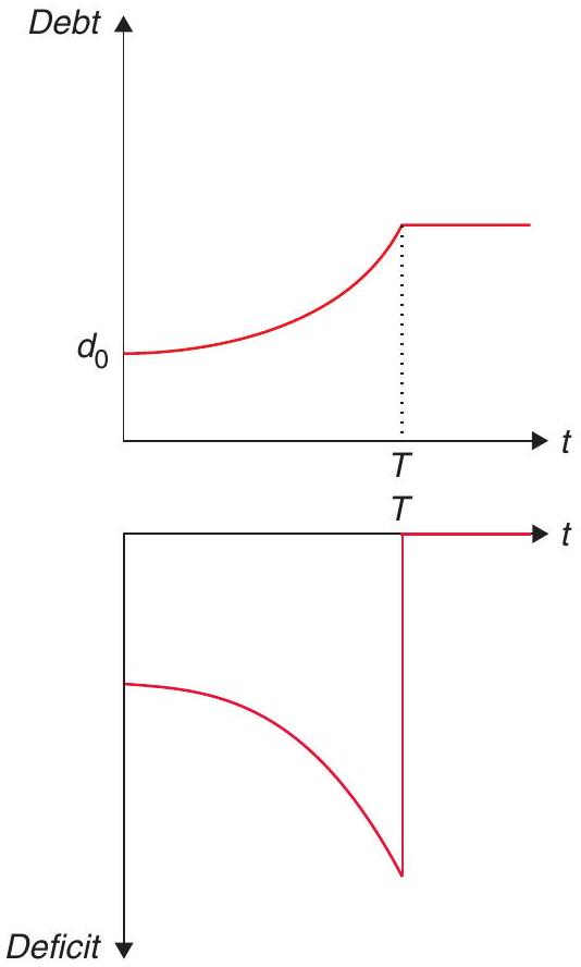
Evaluating (18.1) at time \(T\) we have

\[ \dot{d}_{T}=r d_{T}+g^{L}-\tau^{\prime \prime} . \tag{18.29}\]

Finally, using (18.23) and (18.28) in (18.29) we obtain

\[ \begin{aligned} \dot{d}_{T}= & r d_{0}+\left(1-e^{-r T}\right)\left(g^{H}-g^{L}\right)+g^{L} \\ & -r d_{0}-g^{H}\left(1-e^{-r T}\right)-g^{L} e^{-r T} \\ = & 0 . \end{aligned} \tag{18.30}\]

Hence, debt is constant at time \(T\) and thereafter.

18.1.7 Countercyclical fiscal policy

The pattern we have just established gives us a standard framework for thinking about how fiscal policy should respond to fluctuations: you should run deficits when expenditure needs are unusually high, and compensate with surpluses when they are relatively low. In short, the logic of tax smoothing provides a justification for running a countercyclical fiscal policy, based on long-run intertemporal optimisation.

This basic principle can be even stronger under plausible alternative assumptions, relative to what we have imposed so far. Consider, for instance, the case of a loss function for the deadweight loss of

taxes that depends uniquely on the tax rate (i.e. eliminating the factor \(y_{t}\) that multiplies \(\ell(\cdot)\) in (18.3) above). Then it is easy to see that the FOC is

\[ \ell^{\prime}\left(\frac{\tau_{t}}{y_{t}}\right) \frac{1}{y_{t}}=\lambda, \tag{18.31}\]

which means that the tax rate should be higher in booms and lower in recessions. The same happens if, plausibly, distortions are higher in recessions.² Or if government expenditure has a higher value in recessions than in booms - say, because of unemployment insurance. All of these changes further strengthen the countercyclical nature of fiscal policy.

18.1.8 Smoothing government spending

The opposite happens if there is a desire to smooth government spending over time. Consider, for example, a case where tax revenues are now exogenous, though maybe hit by exogenous shocks. This may capture important cases, such as those in which economies are heavily reliant on the proceeds from natural resources, on whose prices they may not have much influence.³ How should such an economy plan its spending profile?

To discuss this question imagine the case of a country where the government maximises

\[ \int_{0}^{\infty}\left(\frac{\sigma}{1-\sigma}\right) g_{t}^{\frac{\sigma-1}{\sigma}} e^{-\rho t} d t \tag{18.32}\]

subject to the budget constraint:

\[ \dot{b}_{t}=r b_{t}+\tau_{t}+\epsilon_{t}-g_{t}, \tag{18.33}\]

where \(b\) stands for government assets, plus the NPG condition that we omit for brevity. Notice that this is identical to our standard consumption optimisation in an open economy, and, therefore, we know that the government has a desire to smooth government expenditures over time. We assume, though, that the shock to income \(\epsilon_{t}\) follows:

\[ \epsilon_{t}=\epsilon_{0} e^{-\delta t} . \tag{18.34}\]

This embeds a full range of cases - for instance, if \(\delta \rightarrow \infty\) then we have a purely transitory shock, but if \(\delta \rightarrow 0\), the shock would be permanent.

Assuming, for simplicity, as we’ve done before, that \(\rho=r\), the FOC for this problem is \(\dot{g}=0\) : it is now government spending that should remain constant over time. This means that

\[ g=r\left[b_{0}+\frac{\tau}{r}+\frac{\epsilon_{0}}{r+\delta}\right] . \tag{18.35}\]

Notice that the final two terms give the present discounted value of taxes and of the income shock. Using (18.33) in (18.35) (and allowing \(b_{0}=0\) ):

\[ \dot{b}_{t}=\frac{\delta}{r+\delta} \epsilon_{t} . \tag{18.36}\]

Notice that if the shock is permanent \((\delta=0)\), the change in debt is zero, and government spending adjusts immediately to its new level. If shocks are transitory and positive then the government accumulates assets along the converging path. What is the implication of this result? That if the government wants to smooth its consumption, it will actually decrease its expenditures when hit by a negative shock. How persistent the shock is determines the impact on government expenditures. In other words, the desire to smooth this response somewhat weakens the countercyclical results we have discussed above.

18.1.9 Summing up

If taxation is distortionary, then a government should endeavor to smooth the path of taxes as much as possible. That means that taxes respond fully to permanent changes in government expenditure, but only partially to transitory changes. The government borrows in bad times (when its expenditure is unusually high) and repays in good times (when its expenditure is unusually low).

If you think about it, this is exactly the same logic of consumption-smoothing, for the exact same reasons. But it has very important policy consequences: any extraordinary expenditure - e.g. a war, or a big infrastructure project - should be financed with debt, and not with taxes. The path followed by debt, however, ought to satisfy the solvency constraint; in other words, it must be sustainable.

This implies a countercyclical pattern for fiscal policy: you should run deficits when expenditure needs are unusually high, and compensate with surpluses when they are relatively low. This may interact with the business cycle as well: to the extent that spending needs go up in cyclical downturns (e.g. because of unemployment insurance payments), and the revenue base goes up when income goes up, the tax smoothing principle will suggest that deficits increase during recessions, and decrease when times are good. It doesn’t make sense to increase tax rates to deal with higher unemployment insurance needs.

Yet this is different from using fiscal policy as an aggregate demand management tool, which is often the sense in which one may hear the term countercyclical fiscal policy being deployed. That said, there is a clear complementarity between the two angles: running the optimal fiscal policy, from a tax smoothing perspective, will also operate in the right direction when needed for aggregate demand management purposes, to the extent that it has an effect on aggregate demand, as per the previous chapter.

18.2 Other determinants of fiscal policy

We discuss how political considerations may explain why, in practice, we see departures from the tax smoothing prescriptions. We also talk about how rules and institutions might address that.

While tax smoothing is a good starting point to understand and plan fiscal policy, tax smoothing can’t explain many of the observed movements in fiscal policy. What are we missing? Alesina and Passalacqua (2016) provide a comprehensive literature review that you should read to understand the political subtleties of how fiscal policy gets determined in practice. They start by acknowledging that Barro’s tax smoothing theory works very well when it comes to explaining U.S. and UK’s last 200 years of debt dynamics. For these two countries, we see, generally speaking, debt increase during wars and then decline in the aftermath.⁴

More generally, tax smoothing is less descriptively useful when thinking about the short term. First of all, the prescriptions of tax smoothing depend strongly on expectations. When is an increase in spending temporary, thereby requiring smoothing? For a practitioner, it becomes an informed guess at best. Beyond that, however, there are many fiscal episodes that cannot be reconciled with tax smoothing: burgeoning debt-to-GDP ratios, protracted delays in fiscal adjustments, differences in how countries respond to the same shocks, etc.

Such episodes require a political economy story - namely, the realisation that policy makers in practice are not benevolent social planners.⁵ The literature has come up with a menu of alternative possibilities.

18.2.1 The political economy approach

The first of these possibilities relies on the concept of fiscal illusion, which claims that people don’t fully understand the implications of fiscal policy. Voters overestimate the benefits of current expenditure and underestimate the future tax burden. Opportunistic politicians (you?) may take advantage of this. If so, there is a bias towards deficits. A derivation of this theory is the so-called political business cycle literature, which looks at the timing of spending around elections. Even with rational voters, we can still have cycles related to the different preferences of politicians from different parties or ideological backgrounds. There is evidence of electoral budget cycles across countries, but that evidence suggests that they are associated with uninformed voters, and, hence, that they tend to disappear as a democracy consolidates or as transparency increases. The main conclusion is that these factors may explain relatively small and short-lived departures from optimal fiscal policy, but not large and long-lasting excessive debt accumulation.

Another issue has to do with intergenerational redistribution. The idea is that debt redistributes income across generations. Obviously, if there is Ricardian equivalence (for example, because through bequests there are intertemporal links into the infinite future), this is inconsequential. But there are models where this can easily not be the case. For example, imagine a society with poor and rich people. The rich leave positive bequests, but the poor would like to have negative bequests. Because this is not possible, running budget deficits is a way of borrowing on future generations. In this case, the poor vote or push for expansionary fiscal policies. This effect will be stronger the more polarised society is, where the median voter has a lower income relative to average income.

The distributional conflicts may not be across time but actually at the same time. This gives rise to the theory of deficits as the result of distributive conflicts. Alesina and Drazen (1991) kicked off the literature with their model on deficits and wars of attrition. The idea is that whichever group gives in (throws the towel) will pay a higher burden of stabilisation costs. Groups then wait it out, trying to signal their toughness in the hope the other groups will give in sooner. Notice that appointing extremists to fight for particular interest groups can be convenient, though this increases the polarisation of the political system. In this setup, a crisis triggers a stabilisation and fiscal adjustment by increasing the costs of waiting. Drazen and Grilli (1993) show the surprising result that, in fact, a crisis can be welfare enhancing! Laban and Sturzenegger (1994) argue that delays occur because adjustment generates uncertainty, and therefore, there is value in waiting, even if delaying entails costs. Imagine a sick person who fears the risk of an operation to cure his ailment. Under a broad range of parameters, he may choose to wait in the certain state of poor health and put off the chances of an unsuccessful operation. This literature has opened the room to analyse other issues. Signalling, for example, is an important issue. Cukierman and Tommasi (1998) explain that it takes a Nixon to go to China: political preferences opposite to the policies implemented convey more credibly the message of the need for reform (Sharon or Rabin, Lula, etc. are all examples of this phenomenon).

Yet another story related to conflicting preferences about fiscal policy refers to debt as a commitment, or strategic debt. (See Persson and Svensson (1989) and Alesina and Tabellini (1990)). The idea is that a government who disagrees with the spending priorities of a possible successor chooses to overburden it with debt so it restricts its spending alternatives. Then, the more polarised a society, the higher its debt levels. If the disagreement is on the size of government, the low spender will reduce taxes and increase debt. (Does this ring any bells?)

Another version has to do with externalities associated with the provision of local public goods, a version of what is called the tragedy of the commons. Battaglini and Coate (2008) consider a story where a legislature decides on public good provision, but with two kinds of public goods: one that

benefits all citizens equally, and another that is local (i.e. benefits only those who live in the locality where it is provided). If decisions are made by a legislature where members are elected in local districts, an externality arises: a member’s constituents get all the benefits of the bridge their representative got built, but everyone in the country shares in the cost. They show that, in this case, debt will be above the efficient level, and tax rates will be too volatile.

Departures from optimal fiscal policy can also be due to rent-seeking. Acemoglu et al. (2011) or Yared (2010) consider scenarios where there is an agency problem between citizens and self-interested politicians, and the latter can use their informational advantage to extract rents. The tension between the need to provide these incentives to politicians (pushing to higher revenue and lower spending on public goods), on the one hand, and the needs of citizens (lower taxes and higher spending) on the other - and how they fluctuate in response to shocks - can lead to volatility in taxes and overaccumulation of debt.

Finally, an interesting failure of the tax smoothing prediction that is widespread in developing countries is the issue of procyclical fiscal policy. As we have noted, the intuition suggests that fiscal policy should be countercyclical, saving in good times to smooth out spending in bad times. However, Gavin and Perotti (1997) noted that Latin American governments, in particular, have historically tended to do the exact opposite, and the evidence was later extended to show that most developing countries do the same. One explanation is that these countries are credit-constrained: when times are bad, they lose all access to credit, and this prevents them from smoothing. This explanation again begs the question of why these governments don’t save enough so that they eventually don’t need to resort to capital markets for smoothing. Another explanation, proposed by Alesina et al. (2008), builds on a political economy story: in countries with weak institutions and corruption, voters will rationally want the government to spend during booms, because any savings would likely be stolen away. This predicts that the procyclical behaviour will be more prevalent in democracies, where voters exert greater influence over policy, a prediction that seems to hold in the data.

18.2.2 Fiscal rules and institutions

Since there are so many reasons why politicians may choose to depart from optimal fiscal policy prescriptions - and impose costs on society as a result - it is natural to ask whether it might be possible to constrain their behaviour in the direction of optimal policy.

One type of approach in that direction is the adoption of specific rules - the most typical example of which is in the form of balanced-budget requirements. These impose an obvious cost in terms of flexibility: you do want to run deficits and surpluses, as a matter of optimal fiscal policy! The question is whether the political distortions are so large that this may be preferable. One key insight from the literature on such rules is that the costs of adopting them tend to arise in the short run, while the benefits accrue in the longer term. This in itself raises interesting questions about their political sustainability.

You could imagine a variety of rules and institutions, among different dimensions: do you want to decentralise your fiscal decisions? If so, how do you deal with tax sharing? Do you want to delegate decisions to technocrats? Does it all make a difference? The general conclusions is that, even taking into account the endogeneity of institutional arrangements, institutions matter to some extent. Yet there is room for skepticism. After all, many countries have passed balanced-budget rules and yet have never mastered fiscal balance. Chile, on the other hand, had no law, but run a structural, full employment,

1% surplus for many years to compensate for its depletion of copper reserves. In the end, the policy question of how you build credibility is still there: is it by passing a law that promises you will behave, or simply by behaving?

All in all, we can safely conclude that fiscal policy is heavily affected by political factors, which is another reason why the reach of the fiscal instrument as a tool for macroeconomic policy may be blunted in most circumstances. This is particularly so in developing countries, which tend to be more politically (and credit) constrained. As a result, our hunch is that you want transparent, simple, stable (yet flexible), predictable rules for governing fiscal policy. Your success will hinge on convincing societies to stick to these simple rules!

18.3 Optimal taxation of capital in the NGM

We end with a public finance detour: what should be the optimal way of taxing capital in the context of the NGM? We show that even a planner who cares only about workers may choose to tax capital very little. The optimal tax on capital can grow over time, or converge to zero, depending on the elasticity of intertemporal substitution.

Let’s end our discussion of fiscal policy with an application of the NGM. Our exercise will have more the flavour of public finance (what kinds of taxes should we use to fund a given path of government expenditure) rather than the macroeconomic perspective we have focused on so far. We develop it here to show the wealth of questions the framework we have put so much effort to develop throughout the book can help us understand. It will also allow us to present an additional methodological tool: how to solve for an optimal taxation rule.

Imagine that you need to finance a certain amount of public spending within the framework of the NGM. What would be the optimal mix of taxes? Should the central planner tax labour income, or should it tax capital? The key intuition to solving these problems is that the tax will affect behaviour, so the planner has to include this response in his planning problem. For example, if a tax on capital is imposed, you know it will affect the Euler equation for the choice of consumption, so the planner needs to add this modified Euler equation as an additional constraint in the problem. Adding this equation will allow the planner to internalise the response of agents to taxes, which needs to be done when computing the optimal level of taxation.

To make things more interesting, let’s imagine the following setup which follows Judd (1985) and Straub and Werning (2020). There are two types of agents in the economy: capitalists that own capital, earn a return from it, and consume \(C_{t}\); and workers that only have as income their labour, which they consume \(\left(c_{t}\right)\).⁶ We will assume the central planner cares only about workers (it is a revolutionary government!), which is a simplification for exposition. However, we will see that even in this lopsided case some interesting things can happen, including having paths where, asymptotically, workers decide not to tax capitalists!

So let’s get to work. The planner’s problem (in discrete time) would be to maximise

\[ \sum_{t=0}^{\infty}\left(\frac{1}{1+\rho}\right)^{t} u\left(c_{t}\right), \tag{18.37}\]

subject to

\[ u^{\prime}\left(C_{t}\right)=\frac{\left(1+r_{t+1}\right)}{1+\rho}\left(1-\tau_{t+1}\right) u^{\prime}\left(C_{t+1}\right), \tag{18.38}\]

\[ C_{t}+b_{t+1}=\left(1-\tau_{t}\right)\left(1+r_{t}\right) b_{t}, \tag{18.39}\]

\[ c_{t}=w_{t}+T_{t}, \tag{18.40}\]

\[ C_{t}+c_{t}+k_{t+1}=f\left(k_{t}\right)+(1-\delta) k_{t}, \tag{18.41}\]

\[ k_{t}=b_{t} . \tag{18.42}\]

The first equation (18.38) is the Euler condition for capitalists. As we said above, this equation needs to hold and, therefore, has to be considered by the planner as a constraint. The following two equations (18.39) and (18.40) define the budget constraint of capitalists and workers. Capitalist earn income from their capital, though this may be taxed at rate \(\tau\). Workers are just hand-to-mouth consumers: they eat all their income. They receive, however, all the proceeds of the capital tax \(T_{t}=\tau_{t} k_{t}\). Equation (18.41) is the resource constraint of the economy where we assume capital depreciates at rate \(\delta\). Finally equation (18.42) states that in equilibrium the assets of the capitalists is just the capital stock. We have omitted the transversality conditions and the fact that wages and interest rates are their marginal products - all conditions that are quite familiar by now.

Before proceeding you may think that, if the planner cares about workers, and not at all about capitalists, the solution to this problem is trivial: just expropriate the capital and give it to workers. This intuition is actually correct, but the problem becomes relatively uninteresting.⁷ To rule that out, we will add the extra assumption that workers would not know what to do with capital. You actually have to live with the capitalists so they can run the capital.

Something else you may notice is that we have not allowed for labour taxation. Labour taxation creates no distortion here, but would be neutral for workers (what you tax is what you return to them), so the interesting question is what is the optimal tax on capital.

Typically, you would just set out your Bellman equation (or Hamiltonian, if we were in continuous time) to solve this problem, simply imposing the Euler equation of capitalists as an additional constraint. However, if their utility is log, the solution is simpler because we already know what the optimal consumption of capitalists is going to be: their problem is identical to the consumption problem we solved in Chapter 12! You may recall that the solution was that consumption was a constant share of assets \(C_{t}=\frac{\rho}{(1+\rho)}\left(1+r_{t}\right) b_{t}=(1-s)\left(1+r_{t}\right) b_{t}\), where the second equality defines \(s\). Capitalists consume what they don’t save. In our case, this simplifies the problem quite a bit. We can substitute for the capitalists’ consumption in the resource constraint, knowing that this captures the response function of this group to the taxes.⁸ Using the fact that

\[ C_{t}=(1-s)\left(1-\tau_{t}\right)\left(1+r_{t}\right) b_{t}, \tag{18.43}\]

and that

\[ b_{t+1}=s\left(1-\tau_{t}\right)\left(1+r_{t}\right) b_{t}, \tag{18.44}\]

it is easy to show (using the fact that \(b_{t}=k_{t}\) ) that

\[ C_{t}=\frac{(1-s)}{s} k_{t+1} . \tag{18.45}\]

We can replace this in the resource constraint to get

\[ \frac{k_{t+1}}{s}+c_{t}=f\left(k_{t}\right)+(1-\delta) k_{t} . \tag{18.46}\]

Notice that this is equivalent to the standard growth model except that the cost of capital is now increased by \(\frac{1}{s}\). Capital has to be intermediated by capitalists, who consume part of the return, thus making accumulation more expensive from the perspective of the working class.

Solving (18.37) subject to (18.46) entails the first order condition

\[ u^{\prime}\left(c_{t}\right)=\frac{s}{1+\rho} u^{\prime}\left(c_{t+1}\right)\left(f^{\prime}\left(k_{t+1}\right)+1-\delta\right) . \tag{18.47}\]

In steady state, this equation determines the optimal capital stock:

\[ 1=\frac{s}{1+\rho}\left(f^{\prime}\left(k^{*}\right)+1-\delta\right)=s \frac{1}{1+\rho} R^{*} \tag{18.48}\]

where \(R^{*}\) is the interest rate before taxes. Notice that in steady state we must also have that the savings are sufficient to keep the capital stock constant,

\[ s R k=k, \tag{18.49}\]

where \(R\) is the after-tax return for capitalists. Using (18.48) and (18.49), it is easy to see that

\[ \frac{R}{R^{*}}=\frac{1}{1+\rho}=(1-\tau), \tag{18.50}\]

or simply that \(\tau=\frac{\rho}{1+\rho}\).

In short: the solution is a constant tax on capital, benchmarked by the discount rate. In particular, the less workers (or the planner) discount the future, the smaller the tax: keeping the incentives for capitalists to accumulate pays of in the future and therefore is more valuable the less workers discount future payoffs. In the limit, with very patient workers/planner, the tax on capital approaches zero, and this happens even though the planner does not care about the welfare of capitalists! This is a powerful result.

Yet, this result relies heavily on the log utility framework. In fact, Straub and Werning (2020) solve for other cases, and show that things can be quite different. As you may have suspected by now, this is all about income versus substitution effects. Consider a more general version of the utility function of capitalists: \(U\left(C_{t}\right)=\frac{C_{t}^{1-\sigma}}{(1-\sigma)}\). If \(\sigma>1\), the elasticity of intertemporal substitution is low, and income effects dominate. If \(\sigma<1\), in contrast, substitution effects dominate. Does the optimal tax policy change? It does - in fact, Straub and Werning show that, in the first case, optimal taxes on capital grow over time! In the second case, on the other hand, they converge to zero.

The intuition is pretty straightforward: workers want capitalists to save more since, the larger the capital stock, the larger the tax they collect from it. If taxes are expected to increase, and income effects prevail, capitalists will save more in expectation of the tax hike, which makes it optimal from the perspective of the workers to increase taxes over time. The opposite occurs when substitution effects prevail. As we can see, even this simple specification provides interesting and complex implications for fiscal policy.

18.4 What have we learned?

We have seen that, from the standpoint of financing a given path of government spending with a minimum of tax distortions, there is a basic principle for optimal fiscal policy: tax smoothing. Optimal fiscal policy will keep tax rates constant, and finance temporarily high expenditures via deficits, while running surpluses when spending is relatively low. This countercyclical fiscal policy arises not because

of aggregate demand management, but from a principle akin to consumption smoothing. Because high taxes entail severe distortions, you don’t want to have to raise them too high when spending needs arise. Instead, you want to tax at the level you need to finance the permanent level of expenditures, and use deficits and surpluses to absorb the fluctuations.

As it turns out, in practice there are many important deviations from this optimal principle - more often than not in the direction of over-accumulation of debt. We thus went over a number of possible political economy explanations for why these deviations may arise. We can safely conclude that fiscal policy is heavily affected by political factors, which gives rise to the question of whether rules and institutions can be devised to counteract the distortions.

Finally, we briefly went over the public finance question of optimal taxation of capital in the context of the NGM model. We obtained some surprising results - a social planner concerned only with workers may still refrain from taxing capital to induce more capital accumulation, which pays off in the long run. Yet, these results are very sensitive to the specification of preferences, particularly in the elasticity of intertemporal substitution, further illustrating the power of our modelling tools in illuminating policy choices.

18.5 What next?

The survey by Alesina and Passalacqua (2016) is a great starting point for the literature on the determinants of fiscal policy.

References

Acemoglu, D., Golosov, M., & Tsyvinski, A. (2011). Political economy of Ramsey taxation. Journal of Public Economics, 95(7-8), 467-475.

Aiyagari, S. R., Marcet, A., Sargent, T. J., & Seppälä, J. (2002). Optimal taxation without state-contingent debt. Journal of Political Economy, 110(6), 1220-1254.

Alesina, A. & Drazen, A. (1991). Why are stabilizations delayed? American Economic Review, 81(5), 1170-1188.

Alesina, A., Campante, F. R., & Tabellini, G. (2008). Why is fiscal policy often procyclical? Journal of the European Economic Association, 6(5), 1006-1036.

Alesina, A. & Passalacqua, A. (2016). The political economy of government debt. Handbook of Macroeconomics, 2, 2599-2651.

Alesina, A. & Tabellini, G. (1990). A positive theory of fiscal deficits and government debt. The Review of Economic Studies, 57(3), 403-414.

Barro, R. J. (1979). On the determination of the public debt. Journal of Political Economy, 87(5, Part 1), 940-971.

Battaglini, M. & Coate, S. (2008). A dynamic theory of public spending, taxation, and debt. American Economic Review, 98(1), 201-36.

Cukierman, A. & Tommasi, M. (1998). When does it take a Nixon to go to China? American Economic Review, 180-197.

Drazen, A. & Grilli, V. (1993). The benefit of crises for economic reforms. The American Economic Review, 83(3), 598-607.

Gavin, M. & Perotti, R. (1997). Fiscal policy in Latin America. NBER Macroeconomics Annual, 12, 11-61. https://www.journals.uchicago.edu/doi/pdf/10.1086/654320.

Judd, K. L. (1985). Redistributive taxation in a simple perfect foresight model. Journal of Public Economics, 28(1), 59-83.

Laban, R. & Sturzenegger, F. (1994). Distributional conflict, financial adaptation and delayed stabilizations. Economics & Politics, 6(3), 257-276.

Persson, T. & Svensson, L. E. (1989). Why a stubborn conservative would run a deficit: Policy with time-inconsistent preferences. The Quarterly Journal of Economics, 104(2), 325-345.

Straub, L. & Werning, I. (2020). Positive long-run capital taxation: Chamley-Judd revisited. American Economic Review, 110(1), 86-119.

Yared, P. (2010). Politicians, taxes and debt. The Review of Economic Studies, 77(2), 806-840.

---

1. In a model with uncertainty the equivalent to equation (18.10) would be \(\phi_{t}=E\left(\phi_{t+1}\right)\), that is, that the tax rates follow a random walk.

2. A good application of this is to think about the optimal response to the Covid-19 pandemic of 2020. In a forced recession, taxes became almost impossible to pay, in some cases leading to bankruptcies and thus promoting policies of tax breaks during the outbreak.

3. Take the case of Guyana, which one day found oil and saw its revenues grow by 50% in one year - this actually happened in 2020.

4. Even in these countries, however, there are anomalies, such as the U.S. accumulating debt over the relatively peaceful 1980s - more on this later…

5. In fact, the need for a political economy story strikes even deeper. Suppose we had a truly benevolent and farsighted government, what should it do in the face of distortionary taxation? Well, Aiyagari et al. (2002) have the answer: it should accumulate assets gradually, so that, eventually, it would have such a huge pile of bonds that it could finance any level of spending just with the interest it earned from them - no need for any distortionary taxes! In that sense, even the tax smoothing logic ultimately hinges on there being some (binding) upper bound on the level of assets that can be held by the government, often referred to as an ad hoc asset limit.

6. The problem for capitalists is to maximise \(\sum_{t=0}^{\infty}\left(\frac{1}{1+\rho}\right)^{t} u\left(C_{t}\right)\), subject to \(C_{t}+b_{t+1}=\left(1+r_{t}\right) b_{t}\). Notice that this problem is virtually identical, but not exactly the same, to the consumer problem we solved in Chapter 12. The difference is a timing convention. Before savings at time \(t\) did not generate interest income in period \(t\), here they do. Thus what before was \(b_{t}\) will now become \(b_{t}\left(1+r_{t}\right)\).

7. Though in the real world this option sometimes is implemented. Can you think of reasons why we don’t see it more often?

8. The log case is particularly special because the tax rate does not affect the capitalist’s consumption path - more on this in a bit.