16 Unemployment
16.1 Theories of unemployment
One of the most prominent features of the business cycle is the fluctuation in the number of people who are not working. More generally, at any given point in time there are always people who say they would like to work, but cannot find a job. As a result, no book in macroeconomics would be complete without a discussion on what determines unemployment.
The question of why there is unemployment is quite tricky, starting with the issue of whether it exists at all. Every market has frictions, people that move from one job to the next, maybe because they want a change, their business closed, or they were fired. This in-between unemployment is called frictional unemployment and is somewhat inevitable, in the same way that at each moment in time there is a number of properties idle in the real estate market.1
Another difficulty arises when workers have very high reservation wages. This may come about because people may have other income or a safety net on which to rely.2 When this happens, they report to the household survey that they want to work, and probably they want to, but the wage at which they are willing to take a job (their reservation wage) is off equilibrium.3 How should we classify these cases? How involuntary is this unemployment?
Now, when people would like to work at the going wages and can’t find a job, and more so when this situation persists, we say there is involuntary unemployment. But involuntary unemployment poses a number of questions: why wouldn’t wages adjust to the point where workers actually find a job? Unemployed individuals should bid down the wages they offer until supply equals demand, as in any other market. But that does not seem to happen.
Theories of unemployment suggest an explanation of why the labour market may fail to clear. The original Keynesian story for this was quite simple; wages were rigid because people have money illusion, i.e. they confuse nominal with real variables. In that view, there is a resistance to have the nominal wage adjusted downwards, preventing an economy hit by a shock that would require the nominal (and presumably the real) wage to decrease to get there. There may be some truth to the money illusion story4, but economists came to demand models with rational individuals. The money illusion story also has the unattractive feature that wages would be countercyclical, something that is typically rejected in the data.5
The theories of unemployment we will see tell some more sophisticated stories. They can be classified as:
Search/Matching models: unemployment exists as a by-product of the process through which jobs that require different skills are matched with the workers who possess them.
Efficiency-wage theories: firms want to pay a wage above the market-clearing level, because that increases workers’ productivity.
Contracting/Insider-Outsider models: firms cannot reduce the wage to market-clearing levels because of contractual constraints.
We will see that each of these stories (and the sub-stories within each class) will lead to different types of unemployment, for example frictional vs structural. They are not mutually exclusive, and the best way to think about unemployment is having those stories coexist in time and space. To what extent they are present is something that varies with the specific context. Yet, to tackle any of these models, we first need to develop the basic model of job search, to which we now turn.
A word of caution on unemployment data
Unemployment data is typically collected in Permanent Household Surveys. In these surveys, data collectors ask workers if they work (those that answer they do are called employed), if they don’t work and have been looking for a job in the last \(x\) unit of time they are called unemployed. The sum of employed and unemployed workers comprise the labour force. Those that are not in the labour force are out of the labour force (this includes, children, the retired, students, and people who are just not interested in working). The key parameter here is the \(x\) mentioned above. It is not the same to ask about whether you looked for a job in the last minute (unemployment would probably be zero, considering that you are probably answering the survey!), in the last week or in the last year. The longer the span, the higher the labour force and the higher the unemployment rates. Methodological changes can lead to very significant changes in the unemployment figures.
16.2 A model of job search
The theory of search solves the problem faced by an unemployed worker that is faced with random job offers. The solution takes the form of a reservation wage \(w_{R}\). Only if the wage offer is larger than this reservation wage will the searcher take the job.
The specifics of the labour market have motivated the modelling of the process of job search. Obviously, how the market works depends on how workers look for a job. The theory of search tackles this question directly, though later on found innumerable applications in micro and macroeconomics.
Let’s start with the basic setup. Imagine a worker that is looking for a job, and every period (we start in discrete time), is made an offer \(w\) taken from a distribution \(F(w)\). The worker can accept or reject the offer. If he accepts the offer, he keeps the job forever (we’ll give away with this assumption later). If he rejects the offer he gets paid an unemployment compensation \(b\) and gets a chance to try a
new offer the following period. What would be the optimal decision? Utility will be described by the present discounted value of income, which the worker wants to maximise
\[ \mathbb{E} \sum_{t=0}^{\infty} \beta^{t} x_{t}, \tag{16.1}\]
where \(x=w\) if employed at wage \(w\), and \(x=b\) if unemployed and \(\beta=\frac{1}{1+\rho}\). This problem is best represented by a value function that represents the value of the maximisation problem given your current state. For example, the value of accepting an offer with wage \(w\) is
\[ W(w)=w+\beta W(w) . \tag{16.2}\]
It is easy to see why. By accepting the wage \(w\), he secures that income this period, but, as the job lasts forever, next period he still keeps the same value, so the second term is that same value discounted one period. On the other hand, if he does not accept an offer, he will receive an income of \(b\) and then next period will get to draw a new offer. The value of that will be the maximum of the value of not accepting and the value of accepting the offer. Let’s call \(U\) the value of not accepting ( \(U\) obviously is motivated by the word unemployment):
\[ U=b+\beta \int_{0}^{\infty} \max \{U, W(w)\} d F(w) \tag{16.3}\]
Since,
\[ W(w)=w /(1-\beta), \tag{16.4}\]
is increasing in \(w\), there is some \(w_{R}\) for which
\[ W\left(w_{R}\right)=U . \tag{16.5}\]
The searcher then rejects the proposition if \(w<w_{R}\), and accepts it if \(w \geq w_{R}\). Replacing (16.4) in (16.5) gives
\[ U=\frac{w_{R}}{(1-\beta)} . \tag{16.6}\]
But then combining (16.3) and (16.4) with (16.6) we have
\[ \frac{w_{R}}{1-\beta}=b+\frac{\beta}{1-\beta} \int_{0}^{\infty} \max \left\{w_{R}, w\right\} d F(w) \tag{16.7}\]
Subtracting \(\frac{\beta w_{R}}{1-\beta}\) from both sides we get
\[ w_{R}=b+\frac{\beta}{1-\beta} \int_{w_{R}}^{\infty}\left(w-w_{R}\right) d F(w) \tag{16.8}\]
Equation (16.8) is very intuitive. The reservation wage needs to be higher than \(b\), and how much depends on the possibility of eventually obtaining a good match; the better the prospects, the more demanding the searcher will be before accepting a match. On the other hand, a high discount factor, which means that waiting is painful will decrease the reservation wage.
An analogous specification can be built in continuous time. Here the value functions need to be understood as indicating the instantaneous payoff of each state. As time is valuable, these payoffs have to match the interest return of the value function. The analogous of the discrete time version are:
\[ r W(w)=w, \tag{16.9}\]
\[ r U=b+\alpha \int_{0}^{\infty} \max \{0, W(w)-U\} d F(w) . \tag{16.10}\]
Notice how natural the interpretation for (16.9) is. The value of accepting a wage is the present discounted value of that wage \(\frac{w}{r}\). The value of not accepting an offer is the instantaneous payment \(b\) plus \(\alpha\) that needs to be interpreted as the probability with which a new opportunity comes along, times its expected value.6 We can also use our standard asset pricing intuition, which we first encountered when analysing the Hamiltonian. The asset here is the state “looking for a job” that pays a dividend of \(b\) per unit of time. The capital gain (or loss) is the possibility of finding a job, which happens with probability \(\alpha\) and yields a gain of \(\int_{0}^{\infty} \max \{0, W(w)-U\} d F(w)\).
As still \(W\left(w_{R}\right)=U\),
\[ W(w)-U=\left(\frac{w-w_{R}}{r}\right), \tag{16.11}\]
which can be replaced in (16.10) to give an expression for the reservation wage
\[ w_{R}=b+\frac{\alpha}{r} \int_{w_{R}}^{\infty}\left(w-w_{R}\right) d F(w) \tag{16.12}\]
16.2.1 Introducing labour turnover
The model can be easily modified to introduce labour turnover. If the worker can lose his job, we need to introduce in the equation for the value of accepting an offer the possibility that the worker may be laid off and go back to the pool of the unemployed. We will assume this happens with probability \(\lambda\) :
\[ r W(w)=w+\lambda[U-W(w)] . \tag{16.13}\]
The equation for the value of being unemployed remains (16.10), and still \(W\left(w_{R}\right)=U\). Because \(r W\left(w_{R}\right)=w_{R}\) we know that \(r U=w_{R}\). (16.13) implies that \(W(w)=\frac{w+\lambda U}{(r+\lambda)}\), which replacing in (16.10) gives
\[ r U=b+\frac{\alpha}{r+\lambda} \int_{w_{R}}^{\infty}\left[w-w_{R}\right] d F(w) \tag{16.14}\]
or
\[ r W\left(w_{R}\right)=w_{R}=b+\frac{\alpha}{r+\lambda} \int_{w_{R}}^{\infty}\left[w-w_{R}\right] d F(w) . \tag{16.15}\]
The reservation wage falls the higher the turnover; as the job is not expected to last forever, the searcher becomes less picky.
This basic framework constitutes the basic model of functioning of the labour market. Its implications will be used in the remainder of the chapter.
16.3 Diamond-Mortensen-Pissarides model
The Diamond-Mortensen-Pissarides model describes a two-way search problem: that of workers and that of firms. A matching function \(M(U, V)\) that relates the number of matchings to the unemployment and vacancies rates allows us to build a model of frictional unemployment.
We will put our job search value functions to work right away in one very influential way of analysing unemployment: thinking the labour market as a matching problem in which sellers (job-seeking workers) and buyers (employee-seeking firms) have to search for each other in order to find a match. If jobs and workers are heterogeneous, the process of finding the right match will be costly and take time, and unemployment will be the result of that protracted process.7
Let us consider a simple version of the search model of unemployment. The economy consists of workers and jobs. The number of employed workers is \(E\) and that of unemployed workers is \(U\) \((E+U=\bar{L})\); the number of vacant jobs is \(V\) and that of filled jobs is \(F\). (We will assume that one worker can fill one and only one job, so that \(F=E\), but it is still useful to keep the notation separate.) Job opportunities can be created or eliminated freely, but there is a fixed cost \(C\) (per unit of time) of maintaining a job. An employed worker produces \(A\) units of output per unit of time \((A>C)\), and earns a wage \(w\), which is determined in equilibrium. We leave aside the costs of job search, so the worker’s utility is \(w\) if employed or zero if unemployed; the firm’s profit from a filled job is \(A-w-C\), and \(-C\) from a vacant job.
The key assumption is that the matching between vacant jobs and unemployed workers is not instantaneous. We capture the flow of new jobs being created with a matching function
\[ M=M(U, V)=K U^{\beta} V^{\gamma}, \tag{16.16}\]
with \(\beta, \gamma \in[0,1]\). This can be interpreted as follows: the more unemployed workers looking for jobs, and the more vacant jobs available, the easier it will be to find a match. As such, it subsumes the searching decisions of firms and workers without considering them explicitly. Note that we can parameterise the extent of the thick market externalities: if \(\beta+\gamma>1\), doubling the number of unemployed workers and vacant jobs more than doubles the rate of matching; if \(\beta+\gamma<1\) the search process faces decreasing returns (crowding).
We also assume an exogenous rate of job destruction, which we again denote as \(b\). This means that the number of employed workers evolves according to
\[ \dot{E}=M(U, V)-b E . \tag{16.17}\]
We denote \(a\) as the rate at which unemployed workers find new jobs and \(\alpha\) as the rate at which vacant jobs are filled. It follows from these definitions that we will have
\[ a=\frac{M(U, V)}{U}, \tag{16.18}\]
\[ \alpha=\frac{M(U, V)}{V} . \tag{16.19}\]
The above describes the aggregate dynamics of the labor market, but we still need to specify the value for the firm and for the worker associated with each of the possible states. Here is where we will use
the intuitions of the previous section. Using the same asset pricing intuition that we used in (16.9) and (16.10), but now applied to both worker and firm, we can write
\[ r V_{E}=w-b\left(V_{E}-V_{U}\right), \tag{16.20}\]
\[ r V_{U}=a\left(V_{E}-V_{U}\right), \tag{16.21}\]
\[ r V_{V}=-C+\alpha\left(V_{F}-V_{V}\right), \tag{16.22}\]
\[ r V_{F}=A-w-C-b\left(V_{F}-V_{V}\right), \tag{16.23}\]
where \(r\) stands for the interest rate (which we assume to be equal to the individual discount rate). These equations are intuitive, so let’s just review (16.20). The instantaneous value of being employed is the instantaneous wage. With probability \(b\) the worker can become unemployed in which case loses the utility \(\left(V_{E}-V_{U}\right)\). The reasoning behind the other equations is similar, so we can just move on.
We assume that workers and firms have equal bargaining power when setting the wage, so that they end up with the same equilibrium rents:8
\[ V_{E}-V_{U}=V_{F}-V_{V} . \tag{16.24}\]
16.3.1 Nash bargaining
Let us start by computing the rents that will accrue to employed workers and employing firms, as a function of the wage, using (16.20)-(16.23):
\[ r\left(V_{E}-V_{U}\right)=w-b\left(V_{E}-V_{U}\right)-a\left(V_{E}-V_{U}\right) \Rightarrow V_{E}-V_{U}=\frac{w}{a+b+r}, \tag{16.25}\]
\[ r\left(V_{F}-V_{V}\right)=A-w-C-b\left(V_{F}-V_{V}\right)+C-\alpha\left(V_{F}-V_{V}\right) \Rightarrow V_{F}-V_{V}=\frac{A-w}{\alpha+b+r} . \tag{16.26}\]
The assumption of equal bargaining power (16.24) implies that the equilibrium wage must satisfy
\[ \frac{w}{a+b+r}=\frac{A-w}{\alpha+b+r} \Rightarrow w=\frac{(a+b+r) A}{a+\alpha+2 b+2 r} . \tag{16.27}\]
The intuition is simple: \(a\) and \(\alpha\) capture how easy it is for a worker to find a job, and for a firm to find a worker; their relative size determines which party gets the bigger share of output.
The equilibrium will be pinned down by a free-entry condition: firms will create job opportunities whenever they generate positive value. In equilibrium, the value of a vacant job will be driven down to zero. But how much is a vacant job worth to a firm? Using (16.22), (16.26), and (16.27) yields
\[ \begin{aligned} r V_{V}=-C+\alpha & \frac{A-w}{\alpha+b+r}=-C+\alpha \frac{A-\frac{(a+b+r) A}{a+\alpha+2 b+2 r}}{\alpha+b+r} \\ & \Rightarrow r V_{V}=-C+\frac{\alpha}{a+\alpha+2 b+2 r} A . \end{aligned} \tag{16.28}\]
Now recall (16.18) and (16.19). We can turn these into functions of \(E\), by focusing the analysis on steady states where \(E\) is constant. For this to be the case (16.17) implies that \(M(U, V)=b E\), the numbers of jobs filled has to equal the number of jobs lost. It follows that
\[ a=\frac{b E}{U}=\frac{b E}{\bar{L}-E} . \tag{16.29}\]
To find out what \(\alpha\) is, we still need to express \(V\) in terms of \(E\), which we do by using the matching function (16.16):
\[ K U^{\beta} V^{\gamma}=b E \Rightarrow V=\left(\frac{b E}{K U^{\beta}}\right)^{\frac{1}{\gamma}}=\left(\frac{b E}{K(\bar{L}-E)^{\beta}}\right)^{\frac{1}{\gamma}} . \tag{16.30}\]
As a result, we obtain
\[ \alpha=\frac{b E}{V}=\frac{b E}{\left(\frac{b E}{K(\bar{L}-E)^{\beta}}\right)^{\frac{1}{\gamma}}}=K^{\frac{1}{\gamma}}(b E)^{\frac{\gamma-1}{\gamma}}(\bar{L}-E)^{\frac{\beta}{\gamma}} . \tag{16.31}\]
Conditions (16.29) and (16.31) can be interpreted as follows: \(a\) is an increasing function of \(E\) because the more people are employed, the smaller will be the number of people competing for the new job vacancies and the easier it for an unemployed worker to find a job. Similarly, \(\alpha\) is decreasing in \(E\) because the same logic will make it harder for a firm to fill a vacancy.
The final solution of the model imposes the free-entry condition, using (16.28), to implicitly obtain equilibrium employment:
\[ r V_{V}(E)=-C+\frac{\alpha(E)}{a(E)+\alpha(E)+2 b+2 r} A=0 . \tag{16.32}\]
What does the function \(V_{V}(E)\) look like? It is negatively sloped, because
\[ V_{V}^{\prime}(E)=\frac{A}{r} \frac{\alpha^{\prime}(E)[a(E)+2 b+2 r]-a^{\prime}(E) \alpha(E)}{(a(E)+\alpha(E)+2 b+2 r)^{2}}<0 . \tag{16.33}\]
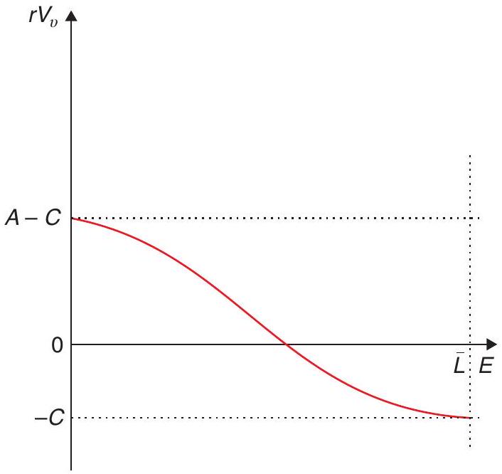
Intuitively, more employment makes it harder and more expensive to fill vacant jobs, reducing their value to the firm. When \(E\) is zero, filling a job is very easy, and the firm gets all the surplus \(A-C\); when \(E\) is equal to \(\bar{L}\) (full employment), it is essentially impossible, and the value of the vacancy is \(-C\). This can be plotted as in Figure 16.1.
16.3.2 Unemployment over the cycle
What happens when there is a negative shock in demand? We can illustrate this through analysing the effect of a drop in \(A\), which a brief inspection of (16.28) shows corresponds to a leftward shift of the \(V_{V}\) curve in Figure 16.1 resulting in an increase in unemployment. Equation (16.27) in turn shows that the equilibrium wage will also fall as a result - though less than one for one, because of the effect of lower employment on the ease and cost of filling new vacancies. This means that the search models generate the kind of cyclical unemployment that characterises recessions.
We can also note that such a decrease in productivity will affect the equilibrium number of vacancies: (16.30) shows that there are fewer vacancies when employment is low. This seems to be consistent with the fact that you don’t see many help wanted signs during recessions. (The negative link between unemployment and vacancies is often called Beveridge curve.) This happens in the model because a steady state with low employment is one in which the matching rate is low, and this means that firms will be discouraged from opening new vacancies that are likely to remain unfilled for a long time. This is precisely due to what is called thick market externalities: if there aren’t many vacancies, people are unlikely to be looking for jobs, which discourages vacancies from being opened. People disregard the effect that their own job search or vacancy has on the thickness of the market, which benefits every other participant.
In any event, the unemployment described in these search models is what we call frictional unemployment - the by-product of the fact that it takes time to match heterogeneous workers and heterogenous jobs. It is hard to think that long-term unemployment of the sort that often happens in real life will be due to this mechanism. Thus, we need other stories to account for a more stable unemployment rate. To these we now turn.
16.4 Efficiency wages
The efficiency wage story builds on the idea that effort increases with wages. The firm may find it optimal to charge an above equilibrium wage to induce workers to exert effort. The chosen wage may lead to aggregate unemployment without firms having an incentive to lower it. Efficiency wages provide then a model of steady state unemployment.
The idea behind efficiency wages is that the productivity of labour depends on effort, and that effort depends on wages. Because of these links, firms prefer to pay a wage that is higher than the market equilibrium wage. But at this wage there is unemployment. The most basic version of this story - one that applies to very poor countries - is that a higher wage makes workers healthier as they can eat better. But there are many other ways to make the argument. For example, it is mentioned that Henry Ford paid his workers twice the running wage to get the best and reduce turnover, and, as we will see in the next section, sometimes firms pay a higher wage to elicit effort because they have difficulty in monitoring workers’ effort.9
To see this, let us consider a general model in which the firm’s profits are
\[ \pi=Y-w L, \]
where
\[ Y=F(e L), \]
with \(F^{\prime}>0\) and \(F^{\prime \prime}<0\). We denote by \(e\) the effort or effectiveness of the worker. The crucial assumption is that this effectiveness is increasing in the real wage:
\[ e=e(w), \]
with \(e^{\prime}>0\). With all these assumption we can rewrite the firm problem as
\[ \operatorname{Max}_{L, w} F(e(w) L)-w L, \]
which has first-order conditions
\[ \frac{\partial \pi}{\partial L}=F^{\prime} e-w=0, \tag{16.34}\]
and
\[ \frac{\partial \pi}{\partial w}=F^{\prime} L e^{\prime}(w)-L=0 . \tag{16.35}\]
Combining (16.34) and (16.35) we have
\[ \frac{w e^{\prime}(w)}{e(w)}=1 . \]
The wage that satisfies this condition is called the efficiency wage. This condition means that the elasticity of effort with respect to wage is equal to one: a 1% increase in the wage translates into an equal increase in effective labour.
Why does this create unemployment? Notice that (16.34) and (16.35) is a system that defines both the wage and employment. If the optimal solution is \(w^{*}\) and \(L^{*}\), total labour demand is \(N L^{*}\) where \(N\) indicates the number of firms. If the supply of labour exceeds this number, there is unemployment because firms will not want to reduce their wages to clear the market.10 We can also extend this model to include the idea that effort depends on the wage the firm pays relative to what other firms pay, or existing labour market conditions. Summers and Heston (1988) do this and the insights are essentially the same.
The model provides an intuitive explanation for a permanent disequilibrium in labour markets. What explains the relation between wages and effort? To dig a bit deeper we need a framework that can generate this relationship. Our next model does exactly that.
16.4.1 Wages and effort: The Shapiro-Stiglitz model
The Shapiro-Stiglitz model builds a justification for efficiency wages on the difficulties for monitoring worker’s effort. Labour markets with little monitoring problems will have market clearing wages and no unemployment. Markets with monitoring difficulties will induce worker’s rents and steady state unemployment.
When you’re at work, your boss obviously cannot perfectly monitor your effort, right? This means you have a moral hazard problem: the firm would like to pay you based on your effort, but it can only observe your production. It turns out that the solution to this moral hazard problem leads to a form of efficiency wages.
Following Shapiro and Stiglitz (1984), consider a model in continuous time with identical workers who have an instantaneous discount rate of \(\rho\) and a utility at any given instant that is given by
\[ u(t)=\left\{\begin{array}{cl} w(t)-e(t) & , \text { if employed } \\ 0 & , \text { otherwise } \end{array}\right. \tag{16.36}\]
where again \(w\) is wage and \(e\) is effort. For simplicity, we assume that effort can take two values, \(e \in\{0, \bar{e}\}\). At any given point in time, the worker can be in one of three states: \(E\) means that she is employed and exerting effort \((e=\bar{e}), S\) means that she is employed and shirking \((e=0)\), and \(U\) denotes unemployment. We assume that there is an exogenous instantaneous probability that the worker will lose her job at any instant, which is given by \(b\). In addition, there is an instantaneous probability \(q\) that a shirking worker will be caught by the firm, capturing the monitoring technology. Finally, the rate at which unemployed workers find jobs is given by \(a\). This is taken to be exogenous by individual agents, but will be determined in equilibrium for the economy as a whole. Firms in this model will simply maximise profits, as given by
\[ \pi(t)=F(\bar{e} E(t))-w(t)[E(t)+S(t)], \tag{16.37}\]
where \(F(\cdot)\) is as before, and \(E(t)\) and \(S(t)\) denote the number of employees who are exerting effort and shirking, respectively.
In order to analyse the choices of workers, we need to compare their utility in each of the states, \(E\), \(S\), and \(U\). Let us denote \(V_{i}\) the intertemporal utility of being in state \(i\); it follows that
\[ \rho V_{E}=(w-\bar{e})+b\left(V_{U}-V_{E}\right) . \tag{16.38}\]
How do we know that? Again, we use our standard asset pricing intuition that we found in the first section of this chapter. The asset here is being employed and exerting effort, which pays a dividend of \(w-\bar{e}\) per unit of time. The capital gain (or loss) is the possibility of losing the job, which happens with probability \(b\) and yields a gain of \(V_{U}-V_{E}\). The rate of return that an agent requires to hold a unit of this asset is given by \(\rho\). Using the intuition that that the total required return be equal to dividends plus capital gain, we reach (16.38). A similar reasoning gives us
\[ \rho V_{S}=w+(b+q)\left(V_{U}-V_{S}\right), \tag{16.39}\]
because the probability of losing your job when shirking is \(b+q\). Finally, unemployment pays zero dividends (no unemployment insurance), which yields11
\[ \rho V_{U}=a\left(V_{E}-V_{U}\right) . \tag{16.40}\]
Solving the model
If the firm wants workers to exert effort, it must set wages such that \(V_{E} \geq V_{S}\). The cheapest way to do that is to satisfy this with equality, which implies
\[ \begin{aligned} V_{E}=V_{S} \Rightarrow(w-\bar{e})+b\left(V_{U}-V_{E}\right)=w+(b+q)\left(V_{U}-V_{S}\right), &\\ \Rightarrow(w-\bar{e})+b\left(V_{U}-V_{E}\right)=w+(b+q)\left(V_{U}-V_{E}\right), &\\ \Rightarrow \bar{e}=q\left(V_{E}-V_{U}\right), &\\ \Rightarrow V_{E}-V_{U}=\frac{\bar{e}}{q}>0 . & \end{aligned} \tag{16.41}\]
Note that wages are set such that workers are strictly better off being employed than unemployed. In other words, firms will leave rents to workers, so they are afraid of losing their jobs and exert effort as a result. What exactly is that wage? We can use (16.38), (16.40) and (16.41) to get
\[ \begin{aligned} \rho V_{E}=(w-\bar{e})-b \frac{\bar{e}}{q}, &\\ \rho V_{U}=a \frac{\bar{e}}{q} . & \end{aligned} \tag{16.42}\]
Subtracting these two equations yields
\[ \rho \frac{\bar{e}}{q}=(w-\bar{e})-b \frac{\bar{e}}{q}-a \frac{\bar{e}}{q} \Rightarrow w=\bar{e}+(\rho+a+b) \frac{\bar{e}}{q} . \tag{16.43}\]
Again this is very intuitive. The wage has to compensate effort, but then adds an extra which depends on the monitoring technology. For example if the monitoring technology is weak, the wage premia needs to be higher.
We know that \(a\) will be determined in equilibrium. What is the equilibrium condition? If we are in steady state where the rate of unemployment is constant, it must be that the number of workers losing their jobs is exactly equal to the number of workers gaining new jobs. If there are \(N\) firms, each one employing \(L\) workers (remember that all workers exert effort in equilibrium), and the total labour supply in the economy is \(\bar{L}\), there are \(a(\bar{L}-N L)\) unemployed workers finding jobs, and \(b N L\) employed workers losing theirs. The equilibrium condition can thus be written as:
\[ a(\bar{L}-N L)=b N L \Rightarrow a=\frac{b N L}{\bar{L}-N L} \Rightarrow a+b=\frac{b \bar{L}}{\bar{L}-N L} . \tag{16.44}\]
Substituting this into (16.43) yields
\[ w=\bar{e}+\left(\rho+\frac{b \bar{L}}{\bar{L}-N L}\right) \frac{\bar{e}}{q} . \tag{16.45}\]
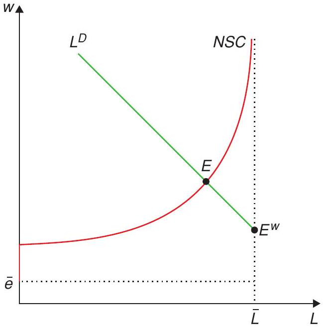
This is the no-shirking condition (NSC), which the wage needs to satisfy in order to get workers to exert effort. Note that \(\frac{\bar{L}-N L}{\bar{L}}\) is the unemployment rate in this economy, so that (16.45) implies that the efficiency wage will be decreasing in the unemployment rate; the greater the unemployment rate is, the more workers will have to fear, and the less their required compensation will be.12 At full employment, an unemployed worker would instantly find a new job just like her old one, so she has nothing to fear from the threat of being fired. The premium is also decreasing in the quality of the monitoring technology, \(q\), which also reduces the need for overcompensation.
We still need to figure out what \(L\) will be in equilibrium. Labor demand by firms will come from the maximisation of (16.37), which entails
\[ \bar{e} F^{\prime}(\bar{e} L)=w . \tag{16.46}\]
A graphic representation of the equilibrium is given in Figure 16.2.
In the absence of the moral hazard problem (or with perfect monitoring), the equilibrium occurs where the labour demand curve crosses the labour supply, which is horizontal at \(\bar{e}\) up until the full employment point \(\bar{L}\), at which it becomes vertical. (The figure assumes that \(\bar{e} F^{\prime}(\bar{e} \bar{L} / N)>\bar{e}\).) This frictionless equilibrium point is denoted \(E^{W}\), and it entails full employment. However, because of the moral hazard problem, the firms will optimally choose to leave rents to workers, which in turn means that some workers will be left unemployed because the wage rate will not go down to market-clearing levels.
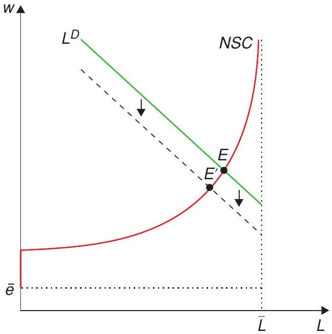
What happens when there is a negative shock to demand? This can be seen in Figure 16.3. We see that unemployment goes up, and the real wage goes down (as higher unemployment makes it cheaper to induce workers’ effort).
Note that this unemployment is inefficient, as the marginal product of labour exceeds the marginal cost of effort. The first-best allocation is for everyone to be employed and to exert effort, but this cannot be simply implemented because of the informational failure.
This model, or rather a simple extension of it, is also consistent with a widespread feature of many labour markets, particularly (but not exclusively) in developing countries: the presence of dual labour markets. Suppose you have a sector where effort can be monitored more easily, say, because output is
less subject to random noise, and another sector (say, the public sector) where monitoring is harder. Then those working in the latter sector would earn rents, and be very reluctant to leave their jobs.
This model has some theoretical difficulties (e.g. Why don’t people resort to more complicated contracts, as opposed to a wage contract? What if the problem is one of adverse selection, e.g. unobservable abilities, as opposed to moral hazard?) and empirical ones (e.g. calibration suggests that the magnitude of employment effects would be quite small). But it is still one of the better-known stories behind efficiency wages.
16.5 Insider-outsider models of unemployment
The insider-outsider story builds an institutional theory of unemployment: unionisation transforms the labour market into a bilateral wage negotiation that may lead to higher than equilibrium wages. The unemployed, however, cannot bid the wage down because they are excluded from the bargaining game.
The insider-outsider model also speaks of a dual labour market, but for different reasons. A standard model of a dual market occurs when governments impose a minimum wage above the equilibrium rate leaving some workers unemployed. Alternatively, in the formal market, unionised workers choose the wage jointly with the firm in a bargaining process. The key assumption is that the firm cannot hire outsiders before it has all insiders (e.g. union members) working, and insiders have little incentive to keep wages low so that outsiders can get a job. As a result the equilibrium wage is higher than the market-clearing wage.
In these dual labour market stories, we may want to ask what is going on in the labour market for outsiders. That, in fact, is a free market, so there should be full employment there. In fact, for most developing countries unemployment is not a big issue, though a privileged number of formal workers do have higher wages. In other words, for the insider-outsider story to generate high economy-wide unemployment, you need the economy to have a very small informal sector. Examples could be European countries or Southern African countries.
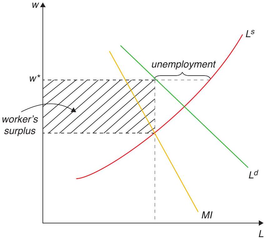
At any rate, to see the insider-outsider story in action as a model of unemployment, consider an economy where all workers are unionised so that aggregate labour demand faces a unique supplier of labour: the centralised union. In Figure 16.4 we show that, as with any monopolist, the price is driven above its equilibrium level, and at the optimal wage there is excess supply of labour (unemployment). Notice that if the demand for labour increases the solution is an increase in the wage and in employment, so the model delivers a procyclical wage.
The role of labour market regulations on the functioning of the labour market is a literature with strong predicament in Europe, where unionisation and labour regulation were more prevalent than, say, in the U.S. In fact, Europe showed historically a higher unemployment rate than the U.S., a phenomenon called Eurosclerosis.
The literature has produced a series of interesting contributions surrounding labour market rigidities. One debate, for example has do to with the role of firing costs on equilibrium unemployment. Increasing firing costs increases or decreases unemployment? It increases unemployment, some would claim because it makes hiring more costly. Others would claim it reduces unemployment because it makes firing more costly. Bentolila and Bertola (1990) calibrated these effects for European labour markets and found that firing costs actually decrease firing and reduce the equilibrium unemployment rate. The debate goes on.
16.5.1 Unemployment and rural-urban migration
Inspired by the slums of Nairobi, which swelled even further as the nation developed, Harris and Todaro (1970) developed the concept that unemployment was a necessary buffer whenever there were dual labour markets. It is a specific version of the insider-outsider interpretation. According to Harris and Todaro, there is a subsistence wage (back in the countryside) ( \(w_{s}\) ) that coexists with the possibility of a job in the formal sector \(\left(w_{f}\right)\). For the market to be in equilibrium, expected wages had to be equalised, i.e.
\[ p w_{f}=w_{s}, \tag{16.47}\]
where \(p\) is the probability of finding a job in the formal sector. How is \(p\) determined? Assuming random draws from a distribution we can assume that
\[ p=\frac{E}{E+U}, \tag{16.48}\]
where \(E\) stands for the total amount of people employed, and \(U\) for the total unemployed. Solving for \(U\), using (16.47) in (16.48) we obtain that
\[ U=E\left(\frac{w_{f}-w_{s}}{w_{s}}\right), \]
i.e. the unemployment rate is a function of the wage differential.
16.6 What next?
The search theory of unemployment is well-covered in Rogerson et al. (2005) Search-Theoretic Models of the Labor Market: A Survey. Two textbooks you need to browse if you want to work on the topics discussed in this chapter are Pissarides (2000) Equilibrium Unemployment Theory and, of course, the graduate level textbook by Cahuc et al. (2014) Labor Economics. This will be more than enough to get you going.
References
Akerlof, G. A. & Yellen, J. L. (1986). Efficiency wage models of the labor market. Cambridge University Press.
Bentolila, S. & Bertola, G. (1990). Firing costs and labour demand: How bad is Eurosclerosis? The Review of Economic Studies, 57(3), 381-402.
Cahuc, P., Carcillo, S., & Zylberberg, A. (2014). Labor economics. MIT Press.
Harris, J. R. & Todaro, M. P. (1970). Migration, unemployment and development: A two-sector analysis. The American Economic Review, 60(1), 126-142.
Lilien, D. M. (1982). Sectoral shifts and cyclical unemployment. Journal of Political Economy, 90(4), 777-793.
Nash Jr, J. F. (1950). The bargaining problem. Econometrica, 155-162.
Pissarides, C. A. (2000). Equilibrium unemployment theory. MIT Press.
Rogerson, R., Shimer, R., & Wright, R. (2005). Search-theoretic models of the labor market: A survey. Journal of Economic Literature, 43(4), 959-988.
Shafir, E., Diamond, P., & Tversky, A. (1997). Money illusion. The Quarterly Journal of Economics, 112(2), 341-374.
Shapiro, C. & Stiglitz, J. E. (1984). Equilibrium unemployment as a worker discipline device. The American Economic Review, 74(3), 433-444.
Summers, R. & Heston, A. (1988). A new set of international comparisons of real product and price levels estimates for 130 countries, 1950-1985. Review of Income and Wealth, 34(1), 1-25.
Lilien (1982) provides evidence that regions in the U.S. with larger sectorial volatility have higher unemployment rates, providing some evidence in favour of the frictional unemployment hypothesis.↩︎
The running joke in the UK in the 70’s claimed that if you were married and had three children you could not afford to be employed. In fact, there is ample evidence that the end of unemployment benefits strongly change the probability of someone finding a job.↩︎
A relevant case of this would be South Africa, which has unemployment rates in the upper 20’s. In South Africa, large portions of the population live in communities far away from city centers, a costly legacy of the Apartheid regime, making commuting costs expensive in money and time. At the same time, large transfers to lower income segments combine with transportation costs to generate large reservation wages. People look for a job but find it difficult to find one that covers these fixed costs, leading to high and persistent unemployment.↩︎
A nice set of empirical experiments showing that nominal illusion is quite pervasive can be found in Shafir et al. (1997).↩︎
Another reason why countercyclical real wages are problematic can be seen with a bit of introspection: if that were the case, you should be very happy during a recession, provided that you keep your job - but that doesn’t seem to be the case!↩︎
Technically, we would call this a hazard rate and not probability, as it is not limited to [0,1]. We abuse our language to aid in the intuition.↩︎
This is but one example of a general kind of problem of two-sided markets, which can be used to study all sorts of different issues, from regulation to poverty traps. The unemployment version was worth a Nobel prize in 2010 for Peter Diamond, Dale Mortensen, and Chris Pissarides, and the analysis of two-sided markets is one of the main contributions of 2014 Nobel laureate Jean Tirole.↩︎
This result is not arbitrarily imposed, but an application of the axiomatic approach to bargaining of Nash Jr (1950).↩︎
Akerlof and Yellen (1986) provide a comprehensive review of the literature on efficiency wages.↩︎
The mathematical intuition for why firms have a low incentive to adjust wages is similar to the argument for the effects of small menu costs under imperfect competition, which we saw in the last handout: because firms are in an interior optimum in the efficiency-wage case, the first-order gains from adjusting wages are zero.↩︎
This assumes that, if employed, the wages will be enough that the worker will want to exert effort, which will be the case in equilibrium.↩︎
This is not unlike the Marxian concept of the reserve army of labor!↩︎