14 Real business cycles
So far we have mostly talked about long-term dynamics, the process of capital accumulation, intergenerational issues, etc. However, a lot of macroeconomics focuses on the short term - the departures from the long-run trend that we’ve been mostly concerned about. This is, of course, particularly evident in recession times! Some of the biggest questions in macroeconomics revolve around this: how can we understand and influence the short-run, cyclical evolution of the economy? What can we (or should we) do about recessions?
These are obviously important questions, and they are very much at the heart of the development of macroeconomics as a discipline, as we discussed in the first chapter of the book. In fact, business cycles is where the distinction between macroeconomic schools of thought became more evident - giving credence to the idea that economists never agree with each other. Many of your policy recommendations will derive from which view of the world you have.
Essentially, one school is ingrained in the Keynesian perspective where there is scope for intervening on the cycle and that doing so is welfare-improving. Its modern version is the New Keynesian approach originated in the 1980s in response to the empirical and methodological challenges from the 1970s. The second approach is quite skeptical about what policy can or should do, as it views the cycle as the result of optimal adjustments to real shocks. Its modern version was born, also in the 1980s, with the so-called Real Business Cycle (RBC) framework, which argued that a perfectly competitive economy, with no distortions or aggregate imbalances of the Keynesian type, but subject to productivity shocks, could largely replicate the business-cycle frequency data for real-world economies.
Recent years have seen a great deal of methodological convergence, with both views adopting, to a large extent, the so-called dynamic stochastic general equilibrium (DSGE) framework that essentially implements the NGM with whatever exogenous shocks and market imperfections that you may feel are relevant. Because this model can be specified to work as a perfectly competitive distortion-free economy, or as one with more Keynesian-type characteristics, it has become the new workhorse of macroeconomics. This has allowed for a more unified conversation in recent decades.
In light of that, and because we have covered much of the ground when we studied the NGM, we will start by describing the RBC framework, which started the trend that turned the NGM into the workhorse of modern macroeconomics. This framework, from a theory standpoint, is, conceptually, a simple extension of the NGM to a context with stochastic shocks.
Yet we will see that it has a sharp message. In particular, it delivers the ultimate anti-Keynesian statement: to the extent that business cycles are optimal responses to productivity shocks, policy interventions are worse than ineffective; they are bad, because they deviate the economy from its intertemporal optimum. From this benchmark, we will then turn to the Keynesian theories.
14.1 The basic RBC model
The basic RBC model is simply the NGM (in discrete time) with two additions: stochastic shocks to productivity (to generate fluctuations in output) and a labour supply choice (to generate fluctuations in employment). Fluctuations come from optimal individual responses to the stochastic shocks.
The basic RBC model, first introduced by Kydland and Prescott (1982), is built around a typical NGM framework of intertemporal maximisation. There are three differences with what we’ve seen so far in the book. First, we introduce uncertainty in the form of exogenous productivity shocks, without which (as we’ve seen) no fluctuations emerge. Second, we also introduce a choice of how much labour will be supplied - in other words, there is a labour-leisure choice. This is what will enable us to say something about fluctuations in employment. Finally, RBC models typically use discrete time. This is so because the objective is to compare the simulated data from the model with that of the real data, which is always discrete, and also because the models quickly become too complicated for analytical solutions. One has to resort to numerical methods of solution, and computers can more easily handle discrete data.
The consumer’s problem works as follows:
\[ \operatorname{Max} E\left[\sum_{t}\left(\frac{1}{1+\rho}\right)^{t}\left((1-\phi) u\left(c_{t}\right)+\phi v\left(h_{t}\right)\right)\right], \tag{14.1}\]
subject to the household budget constraint in which individuals own the capital stock and labour endowment, and rent those out to the firms,
\[ k_{t+1}=l_{t} w_{t}+\left(1+r_{t}\right) k_{t}-c_{t}, \tag{14.2}\]
the production function,
\[ f\left(k_{t}, l_{t}, z_{t}\right)=z_{t} k_{t}^{\alpha} l_{t}^{1-\alpha}, \tag{14.3}\]
the labour endowment equation,
\[ h_{t}+l_{t}=1, \tag{14.4}\]
and a productivity shock process
\[ z_{t+1}=\varphi z_{t}+\varepsilon_{t+1} . \tag{14.5}\]
\(c_{t}\) is consumption, \(h_{t}\) indicates leisure, \(r_{t}\) is the rate of return on capital (net of depreciation), \(k_{t}\) is the capital stock, \(l_{t}\) is the amount of labour devoted to market activities.1 Finally, \(z_{t}\) is a productivity parameter which is subject to random shocks \(\varepsilon_{t}\). The rest are parameters which should be relatively self-explanatory.
14.1.1 The importance of labour supply
As we’ve pointed out, one of the RBC literature’s main departures from the standard NGM is the presence of a labour supply choice. This is crucial to generate fluctuations in employment, which are a pervasive feature of actual business cycles. Let us consider this choice within the context of the basic model. With log utility, the consumer’s objective function can be thought of as:
\[ E\left[\sum_{t}\left(\frac{1}{1+\rho}\right)^{t}\left[(1-\phi) \log \left(c_{t}\right)+\phi \log \left(h_{t}\right)\right]\right] . \]
Notice that the household has two control variables, consumption and leisure. We have seen before the solution to the problem of optimal intertemporal allocation of consumption; it is the familiar Euler equation:
\[ u^{\prime}\left(c_{t}\right)=\frac{1+r_{t+1}}{1+\rho} E\left[u^{\prime}\left(c_{t+1}\right)\right] . \tag{14.6}\]
Leaving aside uncertainty, for the moment, and using the log assumption, we can rewrite this as:
\[ c_{t+1}=\frac{1+r_{t+1}}{1+\rho} c_{t} . \tag{14.7}\]
The labour-leisure choice, in contrast, is static; it takes place in each period with no implication for the next period. The FOC equates the marginal benefit of additional consumption to the marginal cost of lost leisure:
\[ w_{t}(1-\phi) u^{\prime}\left(c_{t}\right)=\phi v^{\prime}\left(h_{t}\right) . \tag{14.8}\]
Again using the log utility assumption, we get
\[ w_{t}(1-\phi) h_{t}=\phi c_{t} . \tag{14.9}\]
To simplify things further, assume for the moment that \(r\) is exogenous - think of a small open economy. In this setup, we can use (14.9) into (14.7) to obtain
\[ \frac{h_{t+1}}{h_{t}}=\frac{1+r}{1+\rho} \frac{w_{t}}{w_{t+1}} \Rightarrow \frac{1-l_{t+1}}{1-l_{t}}=\frac{1+r}{1+\rho} \frac{w_{t}}{w_{t+1}} . \tag{14.10}\]
This means that leisure will be relatively high in those periods when the wage is relatively low; in other words, a higher wage increases the supply of labour. We can also see the impact of the interest rate: a high interest rate will lead to a higher supply of labour. The intuition is that it is worth working more in the present the higher the interest rate, as it provides a higher return in terms of future leisure. These responses of the labour supply, driven by intertemporal substitution in labour and leisure, are at the very heart of the fluctuations in employment in RBC models.
The long-run labour supply
Let’s pause for a minute to explore a bit deeper the shape of this labour supply curve. Consider the case when wages and income are constant, a case that would be akin to analysing the effect of permanent shocks to these variables. Let’s see the form of the labour supply in this case.
Since consumption is constant at income level
\[ c_{t}=w\left(1-h_{t}\right), \tag{14.11}\]
substituting this into (14.8) we obtain
\[ (1-\phi) u^{\prime}\left(w\left(1-h_{t}\right)\right)=\frac{\phi v^{\prime}\left(h_{t}\right)}{w} . \tag{14.12}\]
Using the log specification for consumption and allowing for \(\phi=\frac{2}{3}\) allows us to simplify
\[ \left(\frac{1}{3}\right) \frac{1}{w\left(1-h_{t}\right)}=\frac{2}{3} \frac{1}{w h_{t}}, \tag{14.13}\]
\[ \frac{1}{\left(1-h_{t}\right)}=\frac{2}{h_{t}} \Rightarrow h_{t}=\frac{2}{3} . \tag{14.14}\]
This is a strong result that says that leisure is independent of the wage level. You may think this is too strong but, surprisingly, it fits the data very well, at least when thinking about labour supply in the very, very long run.2 It does seem that for humans income and substitution effects just cancel out (or maybe you prefer a more Leontieff setup in which people just can’t work more than eight hours per day, or where the disutility of labour beyond eight hours a day becomes unbearable if repeated every day).
Does this mean that labour supply does not move at all? Not really. The above was derived under the assumption of the constancy of the wage. This is akin to assuming that any change in wages is permanent, which induces a very large response in the shadow value of consumption that works to offset the labour supply effect of the change in wages (totally cancelling it in the log case). But if the wage moves for a very short period of time we can assume the shadow value of consumption to remain constant, and then changes in the wage will elicit a labour supply response. Thus, while the long-run elasticity of labour supply may be zero, it is positive in the short run.
The basic mechanics
In its essence, the RBC story goes as follows: consider a positive productivity shock that hits the economy, making it more productive. As a result of that shock, wages (i.e. MPL) and interest rates (i.e. MPK) go up, and individuals want to work more as a result. Because of that, output goes up. It follows that the elasticity of labour supply (and the closely related elasticity of intertemporal substitution) are crucial parameters for RBC models. One can only obtain large fluctuations in employment, as needed to match the data, if this elasticity is sufficiently high. What is the elasticity of labour supply in this basic model? Consider the case when \(\frac{(1+r)}{(1+\rho)}=1\), in which consumption is a constant. We can read (14.8) as implying a labour supply curve (a relation between \(l_{t}\) and \(w_{t}\) ):
\[ \phi v^{\prime}\left(1-l_{t}\right)=\lambda w_{t}, \tag{14.15}\]
where \(\lambda\) is the (constant) marginal utility of consumption. Let’s assume a slightly more general, functional form for the utility of leisure:
\[ v(h)=\frac{\sigma}{1-\sigma} h^{\frac{\sigma-1}{\sigma}}, \tag{14.16}\]
plugging this in (14.15) gives
\[ \phi h_{t}^{-\frac{1}{\sigma}}=\lambda w_{t} \tag{14.17}\]
or
\[ h_{t}=\left(\frac{\lambda w_{t}}{\phi}\right)^{-\sigma}, \tag{14.18}\]
which can be used to compute the labour supply:
\[ l_{t}=1-\left(\frac{\lambda w_{t}}{\phi}\right)^{-\sigma} . \tag{14.19}\]
This equation has a labour supply elasticity in the short run equal to
\[ \frac{d l}{d w} \frac{w}{l}=\varepsilon_{l, w}=\frac{\sigma\left(\frac{\lambda w_{t}}{\phi}\right)^{-\sigma-1}\left(\frac{\lambda w_{t}}{\phi}\right)}{1-\left(\frac{\lambda w_{t}}{\phi}\right)^{-\sigma}}=\frac{\sigma\left(\frac{\lambda w_{t}}{\phi}\right)^{-\sigma}}{1-\left(\frac{\lambda w_{t}}{\phi}\right)^{-\sigma}}=\frac{\sigma h_{t}}{l_{t}} . \tag{14.20}\]
If we assume that \(\sigma=1\) (logarithmic utility in leisure), and that \(\phi\) and \(\lambda\) are such that \(\frac{h}{l}=2\) (think about an 8-hour workday), this gives you \(\varepsilon_{l, w}=2\). This doesn’t seem to be enough to replicate the employment fluctuations observed in the data. On the other hand, it seems to be quite high if compared to micro data on the elasticity of labour supply. Do you think a decrease of 10% in real wages (because of inflation, for instance) would lead people to work \(20 \%\) fewer hours?
14.1.2 The indivisible labour solution
The RBC model thus delivers an elasticity of labour supply that is much higher than what micro evidence suggests, posing a challenge when it comes to matching real-world fluctuations in employment. One proposed solution for the conundrum is to incorporate the fact that labour decisions are often indivisible. This means that people may not make adjustments so much on the intensive margin of how many hours to work in your job, but more often on the extensive margin of whether to work at all. This implies that the aggregate elasticity is large even when the individual elasticity is small.
Hansen (1985) models that by assuming that there are fixed costs of going to work. This can actually make labour supply very responsive for a range of wage levels. The decision variables are both days of work: \(d \leq \bar{d}\), and, then, the hours of work each day: \(n\). We assume there is a fixed commuting cost in terms of utility \(\kappa\), which you pay if you decide to work on that day, regardless of how many hours you work (this would be a sort of commuting time).
The objective function is now
\[ \operatorname{MaxE}\left[\sum_{t}\left(\frac{1}{1+\rho}\right)^{t}\left[u\left(c_{t}\right)-d_{t} v\left(n_{t}\right)-\kappa_{t} d_{t}\right]\right], \tag{14.21}\]
where we leave aside the term \(\phi\) to simplify notation, and abuse notation to have \(v(\cdot)\) be a function of hours worked, rather than leisure, entering negatively in the utility function. The budget constraint is affected in that now wage income is equal to \(w_{t} d_{t} n_{t}\).
It is easy to see that we have the same FOCs, (14.7) - which is unchanged because the terms in consumption in both maximand and budget constraint are still the same -, and (14.8) - because the term in \(n_{t}\) is multiplied by \(d_{t}\) in both maximand and budget constraint, so that \(d_{t}\) cancels out. What changes is that now we have an extra FOC with respect to \(d_{t}\) :
\[ \left[v\left(n_{t}\right)+k_{t}\right] \geq u^{\prime}\left(c_{t}\right) w_{t} n_{t} . \tag{14.22}\]
Assume \(\frac{(1+r)}{(1+\rho)}=1\), so that \(c_{t}\) is constant. Then (14.8) simplifies to
\[ v^{\prime}\left(n_{t}\right)=\lambda w_{t} \Longrightarrow n^{*}(w), \tag{14.23}\]
which gives the optimal amount of hours worked (when the agent decides to work). Then (14.22) simplifies to
\[ v\left(n^{*}\right)+k_{t} \geq \lambda w_{t} n^{*} . \tag{14.24}\]
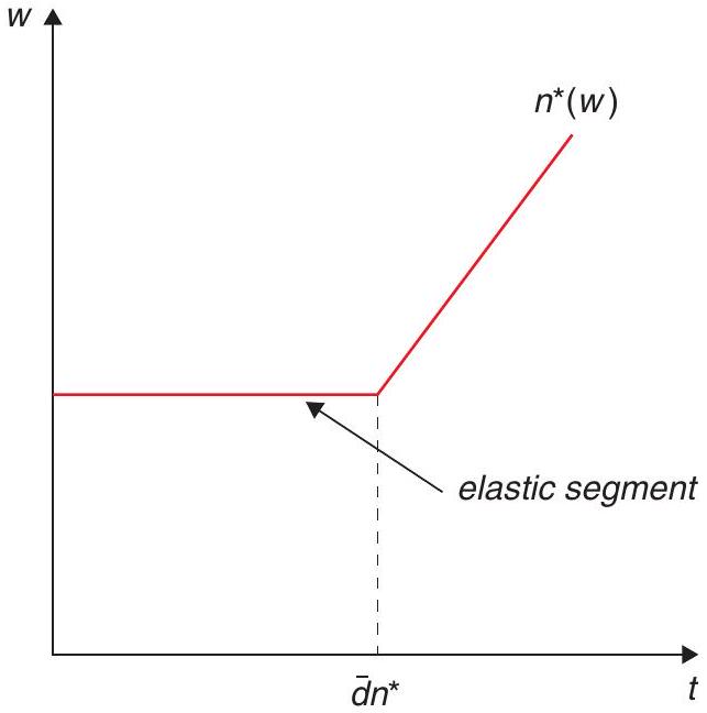
If \(v\left(n^{*}\right)+k>\lambda w n^{*}\), then \(d=0\), otherwise \(d=\bar{d}\). This gives rise to a labour supply as shown in Figure 14.1
The important point is that this labour supply curve is infinitely elastic at a certain wage. The intuition is that on the margin at which people decide whether to work at all or not, the labour supply will be very sensitive to changes in wages.3
14.2 RBC model at work
RBC models typically cannot be solved analytically, and require numerical methods. We discuss an example of a calibration approach to assess the success of the model in describing actual economic fluctuations.
Having discussed the basic intuition behind generating output and employment fluctuations from real shocks to the economy, let us now talk a little bit more generally about how RBC models are usually handled. The main challenge is that even simple specifications are impossible to solve analytically, so the alternative is to use numerical methods.
How is this done? In a nutshell, the strategy is to solve for the FOCs of the model which, in addition to the equations determining the nature of the stochastic shocks, will describe the dynamic path of the variables of interest. (This will often imply a step in which the FOCs are log-linearised around the balanced growth path, since it is easiest to analyse the properties of a linear system.) We then need to provide numbers for the computer to work with - this is done by calibrating the parameters. (Remember what we have discussed of calibration when talking about growth empirics - this approach was pretty much pioneered by the RBC literature.) Because the model is calibrated on the basis of parameters that are brought from “outside the model”, the procedure provides somewhat of an independent test of the relevance of the model.
With this in hand, the model is simulated, typically by considering how the variables of interest responds after being exposed to a stochastic draw of exogenous productivity shocks. The results are then compared to the data. In both cases, the simulated and the real data, we work with the business cycle component, i.e. detrending the data. This is usually done using the Hodrick-Prescott filter, which is a statistical procedure to filter out the trend component of a time series. What output of the model is then compared to the data? Mostly second moments: variances and covariances of the variables of interest. A model is considered successful if it matches lots of those empirical moments.
14.2.1 Calibration: An example
Let us consider the basic RBC model, and the calibration proposed by Prescott (1986) which is the actual kick-off of this approach and where Prescott tackles the issue of assigning parameters to the coefficients of the model. For example, at the time, he took as good a capital share of \(\alpha=0.36\).4 To estimate the production function, he starts with a Cobb-Douglas specification we’ve used repeatedly
\[ f(k)=k^{\alpha} . \tag{14.25}\]
Remember that the interest rate has to equal the marginal product of capital,
\[ f^{\prime}(k)=\alpha k^{\alpha-1}, \tag{14.26}\]
which means that we have an equation for the return on capital:
\[ r=\alpha \frac{Y}{K}-\delta . \tag{14.27}\]
Now let’s put numbers to this. What is a reasonable rate of depreciation? Let’s use (14.27) itself to figure it out. If we assume that the rate of depreciation is \(10 \%\) per year (14.27) becomes
\[ 0.04=0.36 \frac{Y}{K}-0.10 \tag{14.28}\]
\[ 0.14=0.36 \frac{Y}{K} \tag{14.29}\]
\[ \frac{0.36}{0.14}=\frac{K}{Y}=2.6 . \tag{14.30}\]
This value for the capital output ratio is considered reasonable, so the 10% rate of depreciation seems to be a reasonable guess.
How about the discount factor? It is assumed equal to the interest rate. (This is not as restrictive as it may seem, but we can skip that for now.) This implies a yearly discount rate of about \(4 \%\) (the real interest rate), so that \(\frac{1}{1+\rho}=0.96\) (again, per year).
As for the elasticity of intertemporal substitution, he argues that \(\sigma=1\) is a good approximation, and uses the share of leisure equal to \(2 / 3\), as we had anticipated (this gives a labour allocation of half, which is reasonable if we consider that possible working hours are 16 per day).
Finally, the productivity shock process is derived from Solow-residual-type estimations (as discussed in Chapter 6 when we talked about growth accounting), which, in the case of the U.S. at the time, yielded:
\[ z_{t+1}=0.9 * z_{t}+\varepsilon_{t+1} . \tag{14.31}\]
This is a highly persistent process, in which shocks have very long-lasting effects. The calibration for the standard deviation of the disturbance \(\varepsilon\) is 0.763.
So, endowed with all these parameters, we can pour them into the specification and run the model over time - in fact, multiple times, with different random draws for the productivity shock. This will give a time series for the economy in the theoretical model. We will now see how the properties of this economy compare to those of the real economy.
14.2.2 Does it work?
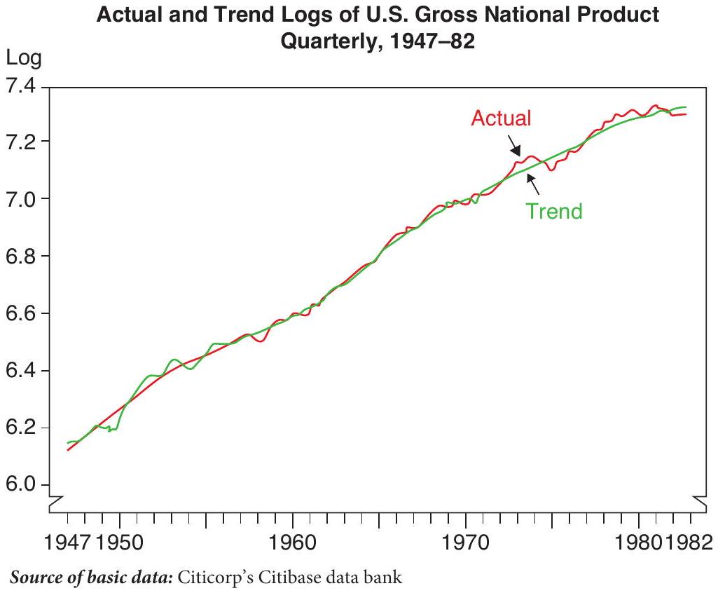
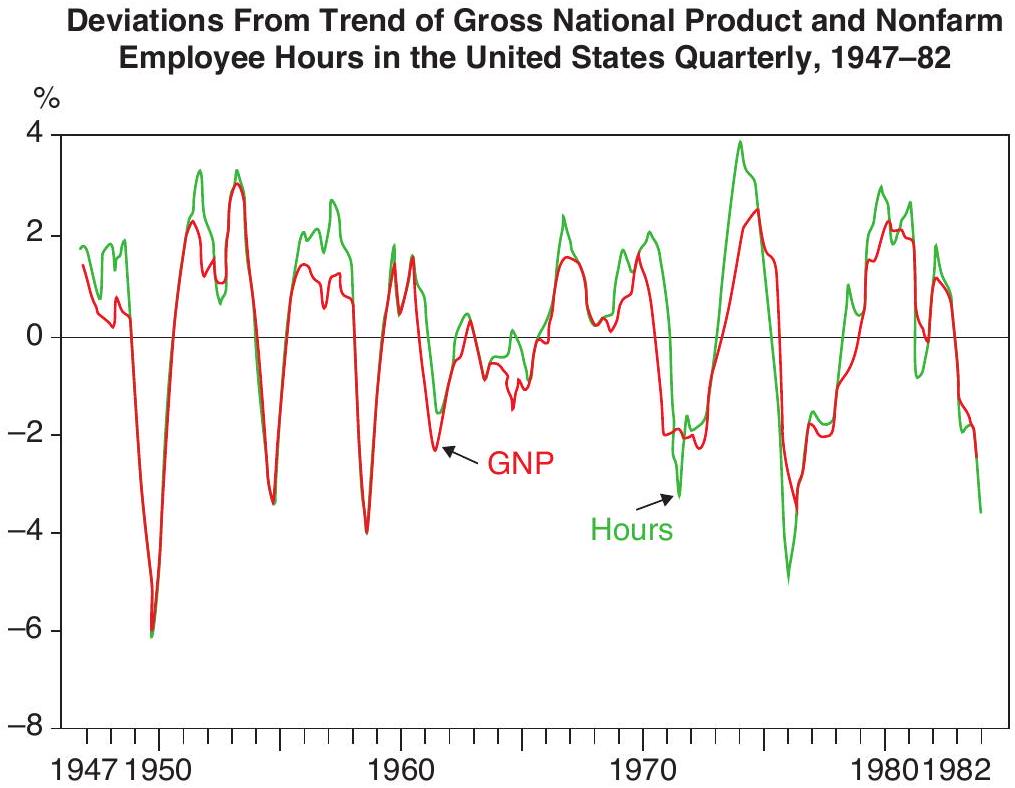
Let’s start with some basic results taken directly from Prescott’s paper. Figure 14.2 shows log U.S. GDP and its trend. The trend is computed as a Hodrick-Prescott filter (think of this as a smoothed, but not fixed, line tracing the data). It is not a great way to compute the business cycle (particularly at the edges of the data set), but one that has become quite popular. Once the trend is computed, the cycle is easily estimated as the difference between the two and is showing in figure 14.3.
Figure 14.3 also shows the variation over the cycle in hours worked. As you can see, there is a large positive correlation between the two.
Real business cycle papers will typically include a table with the properties of the economy, understood as the volatility of the variables and their cross-correlation over time. Table 14.1 and 14.2 show this from Prescott’s original paper for both the real data and the calibrated model.
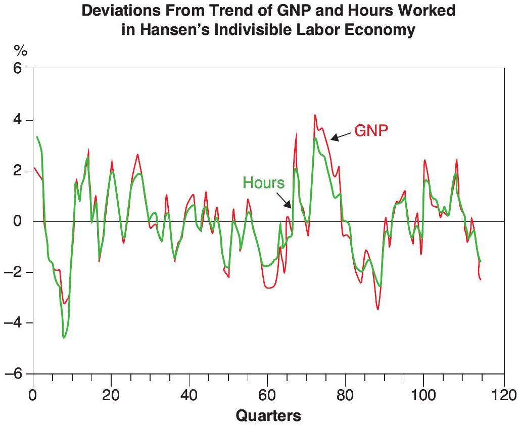
As you can see, things work surprisingly well in the sense that most characteristics of the economy match. The volatility of output and the relative volatility of consumption and investment appear to be the optimal response to the supply shocks. The only caveat is that hours do not seem to move as much as in the data. This is why Prescott implemented Hansen’s extension. Figure 14.4 shows how labour and output move in the Hansen economy (they seem to match better the pattern in Figure 14.1).
The Appendix to this chapter (at the end of the book) will walk you through an actual example so that you learn to numerically solve and simulate an RBC-style model yourself!
Source of basic data: Citicorp’s Citibase data bank
| Cyclical Behavior of the U.S. Economy Deviations From Trend of Key Variables. 1954:1-1982:4 | ||||
|---|---|---|---|---|
| Variable \(\boldsymbol{x}\) | Standard Deviation | Cross Correlation of GNP With | ||
| \(\boldsymbol{x} \boldsymbol{(} \boldsymbol{t} \boldsymbol{-} \mathbf{1} \boldsymbol{)}\) | \(\boldsymbol{x} \boldsymbol{(} \boldsymbol{t} \boldsymbol{)}\) | \(\boldsymbol{x} \boldsymbol{(} \boldsymbol{t} \boldsymbol{+} \mathbf{1} \boldsymbol{)}\) | ||
| Gross National Product | 1.8% | . 82 | 1.00 | . 82 |
| Personal Consumption Expenditures | ||||
| Services | . 6 | . 66 | . 72 | . 61 |
| Nondurable Goods | 1.2 | . 71 | . 76 | . 59 |
| Fixed investment Expenditures | 5.3 | . 78 | . 89 | . 78 |
| Nonresidential Investment | 5.2 | . 54 | . 79 | . 86 |
| Structures | 4.6 | . 42 | . 62 | . 70 |
| Equipment | 6.0 | . 56 | . 82 | . 87 |
| Capital Stocks | ||||
| Total Nonfarm Inventories | 1.7 | . 15 | 4.8 | . 68 |
| Nonresidential Structures | . 4 | -. 20 | -. 03 | . 16 |
| Nonresidential Equipment | 1.0 | . 03 | . 23 | . 41 |
| Labor Input | ||||
| Nonfarm Hours | 1.7 | . 57 | . 85 | . 89 |
| Average Weekly Hours in Mfg. | 1.0 | . 76 | . 85 | . 61 |
| Productivity (GNP/Hours) | 1.0 | . 51 | . 34 | -. 04 |
Source of basic data: Citicorp’s Citibase data bank
| Cyclical Behavior of the Kydland-Prescott Economy* | ||||
|---|---|---|---|---|
| Variable \(x\) | Standard Deviation | Cross Correlation of GNP With | ||
| \(x(t-1)\) | \(\boldsymbol{x} \boldsymbol{(} \boldsymbol{t} \boldsymbol{)}\) | \(x(t+1)\) | ||
| Gross National Product | 1.79% (.13) | . 60 (.07) | 1.00 (-) | . 60 (.07) |
| Consumption | . 45 (.05) | . 47 (.05) | . 85 (.02) | . 71 (.04) |
| Investment | 5.49 (.41) | . 52 (.09) | . 88 (.03) | . 78 (.03) |
| Inventory Stock | 2.20 (.37) | . 14 (.14) | . 60 (.08) | . 52 (.05) |
| Capital Stock | . 47 (.07) | -. 05 (.07) | . 02 (.06) | . 25 (.07) |
|---|---|---|---|---|
| Hours | 1.23 (.09) | . 52 (.09) | . 95 (.01) | . 55 (.06) |
| Productivity (GNP/Hours) | . 71 (.06) | . 62 (.05) | . 86 (.02) | . 56 (.10) |
| Real Interest Rate (Annual) | . 22 (.03) | . 65 (.07) | . 60 (.20) | . 36 (.15) |
*These are the means of 20 simulations, each of which was 116 periods song. The numbers parentheses are standard errors.
Source: Kydland and Prescott 1984
Source: Gray D. Hansen, Department of Economics, University of California, Santa Barbara
14.3 Assessing the RBC contribution
The RBC approach led to a methodological revolution in macroeconomics; all macro models from then on have been expected to be framed as a dynamic stochastic general-equilibrium model with fully optimising agents and rational expectations. Whether or not you buy it as an explanation for business cycle fluctuations in general, and the associated critique of policy interventions, the approach can be useful in understanding at least some aspects of actual fluctuations.
Prescott (1986) summarises the claim in favour of the RBC model: “Economic theory implies that, given the nature of the shocks to technology and people’s willingness and ability to intertemporally and intratemporally substitute, the economy will display fluctuations like those the U.S. economy displays.” His claim is that his model economy matches remarkably well the actual data and, to the extent that it doesn’t, it’s probably because the real-world measurement does not really capture what the theory says is important - hence the title of ’Theory Ahead of Business Cycle Measurement’.
The startling policy implications of these findings are highlighted as follows: “Costly efforts at stabilization are likely to be counterproductive. Economic fluctuations are optimal responses to uncertainty in the rate of technological change.” In other words, business cycle policy is not only useless, but harmful. One should focus on the determinants of the average rate of technological change.
The macro literature has vigorously pursued and refined the path opened by Prescott. Lots of different changes have been considered to the original specification, such as different sources for the shocks (for instance, government spending) or the inclusion of a number of market distortions (e.g. taxation). On the other hand, many objections have been raised to the basic message of RBCs. Do we really see such huge shifts in technology on a quarterly basis? Or, is the Solow residual capturing something else? (Remember, it is the measure of our ignorance…) Do we really believe that fluctuations are driven by people’s willingness to intertemporally reallocate labour? If these are optimal, why do they feel so painful? How about the role of monetary policy, for which the RBC model has no role? Finally, it seems that the features of the fluctuations that are obtained are very close to the nature of the stochastic process that is assumed for the shocks - how much of an explanation is that?
Kydland and Prescott eventually received the Nobel Prize in Economics in 2004, partly for this contribution. (We will return to other contributions by the pair when we discuss monetary policy.) More importantly, the approach led to two developments. First, it generated a fierce counterattack to Keynesianism. The rational expectations revolution had stated that Keynesian policy was ineffective; Kydland and Prescott said it was wrong and harmful. Second, by validating the model, this calibrated stochastic version of the NGM became the workhorse of macroeconomics, so that the RBC approach won the methodological contest. In macro these days, people are pretty much expected to produce a DSGE model with fully optimising agents (with rational expectations) that is amenable to the discipline of calibration. Even the folks who believe in Keynesian-style business cycles are compelled to frame them in such models, though including some price rigidity, monetary disturbance, and so on, as we will see soon.
In addition, even if you believe that the Keynesian approach is a better description of business cycles in general, it may still be the case that a simple RBC framework can explain some important economic episodes. For instance, take a look at Figure 14.5, which depicts GDP, employment, consumption, and investment data for the U.S. over 2019-20. The sharp drop we see is, of course, the economic response to the Covid-19 pandemic, which fits well the supply shock paradigm. The response looks a lot like the kind of logic we have seen in this chapter: a shock to productivity - in this case, the threat posed by a virus - radically changes the intertemporal tradeoff, and leads to a postponement of labour supply and, consequently, to drops in employment and output. Notice that consumption in this case is not smoother than output even though investment is the most volatile variable, as the model predicts. Why is consumption more volatile in this context? Eichenbaum et al. (2020) provide an explanation. They make the realistic assumption that during the Covid-19 pandemic, people attached a risk of contagion to the act of consuming (consumption means going out to a restaurant, shopping mall, etc.) and, therefore, reduced consumption more than they would have done if only adjusting for the change in intertemporal wealth. The example illustrates that some specific changes in the setup may be required on occasion to adjust empirical observations.5
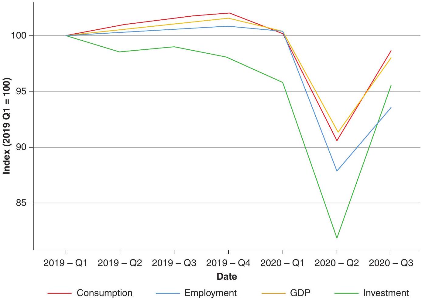
This particular example illustrates that real shocks actually exist, and shows, more broadly, that you do not have to be an RBC true believer to accept that the logic they illuminate has practical applications.
14.4 What have we learned?
The RBC approach to business cycle fluctuations is conceptually very straightforward; take the basic NGM model, add productivity shocks (and a labour-supply choice), and you will get business cycle fluctuations. It highlights the importance of intertemporal substitution and labour supply elasticities as important potential driving factors behind these fluctuations, and can provide a useful lens with which to understand real-world fluctuations, at the very least, in some circumstances (as illustrated by the case of the Covid-19 pandemic).
The approach also has a very sharp message in terms of policy: you should not pursue countercyclical policy. If fluctuations are simply the optimal response of a distortion-free economy to real shocks, policy would only add noise to the process, and make adjustments harder. As we will see, the Keynesian approach has a very different, more policy-friendly message. The contraposition of these two traditions - and particularly the role they assign to policy intervention - is very much at the heart of macroeconomic policy debates.
But we also learned that, underpinning this policy divergence, is a substantial degree of methodological convergence. All of mainstream modern macroeconomics, to a first approximation, speaks
the language that was first introduced by the RBC approach - that of dynamic, stochastic general equilibrium (DSGE) models.
14.5 What next?
Readers who are interested in the RBC approach can go to McCandless (2008), The \(A B C s\) of \(R B C s\), which, as the title indicates, provides a simple and practical introduction to solving RBC models. The paper by Prescott (1986) is also worth reading, as it provides a veritable manifesto of the original approach.
Those who want to dig deeper into the type of recursive methods that have become ubiquitous in macroeconomics, to solve models in the methodological tradition inaugurated by the RBC approach, should look into Ljungqvist and Sargent (2018). You will actually see many of the themes that we discuss in this book, but presented at a whole other level of formal rigor.
References
Chetty, R., Guren, A., Manoli, D., & Weber, A. (2011). Are micro and macro labor supply elasticities consistent? A review of evidence on the intensive and extensive margins. American Economic Review, 101(3), 471-75.
Eichenbaum, M. S., Rebelo, S., & Trabandt, M. (2020). The macroeconomics of epidemics (tech. rep.). National Bureau of Economic Research.
Hansen, G. D. (1985). Indivisible labor and the business cycle. Journal of Monetary Economics, 16(3), 309-327.
Kydland, F. E. & Prescott, E. C. (1982). Time to build and aggregate fluctuations. Econometrica, 1345-1370.
Ljungqvist, L. & Sargent, T. J. (2018). Recursive macroeconomic theory. MIT Press.
McCandless, G. (2008). The ABCs of RBCs. Cambridge, Massachusetts, London: Harvard.
Parente, S. L. & Prescott, E. C. (2002). Barriers to riches. MIT Press.
Prescott, E. C. (1986). Theory ahead of business-cycle measurement. Carnegie-Rochester Conference Series on Public Policy, 25, 11-44.
Sturzenegger, F. (2020). Should we hibernate in a lockdown? Economics Bulletin, 40(3), 2023-2033.
You will often see \(l\) used to refer to leisure and \(n\) to labour, but we are going to stick with \(l\) for labour, for consistency. Think about \(h\) as standing for holidays.↩︎
One way to think about this is asking yourself the following question: how many times higher are real wages today than, say, 300 years ago? And how many more hours do we work?↩︎
Here is a weird little prediction from this model: note that consumption is constant regardless of the employment decision. This means that unemployed and employed workers have the same consumption. But, since work generates disutility, that means that unemployed workers are better off! For a discussion on the state-of-the-art of this debate, see Chetty et al. (2011).↩︎
Remember that Parente and Prescott (2002) argue for \(\alpha=.66\), but this was later…↩︎
An alternative story is provided by Sturzenegger (2020). In his specification, utility changes and people, due to lockdowns, require fewer goods to obtain the same utility. The result is a sharp fall in optimal consumption as in Eichenbaum et al. (2020).↩︎