3. An Overview of Long-Run Economic Growth

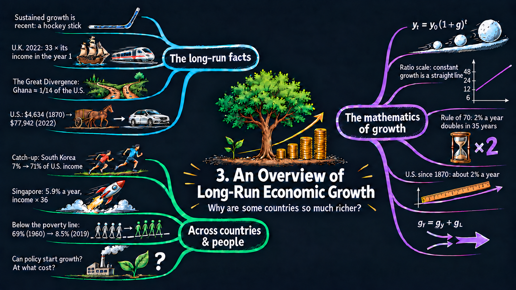
Learning goals

This chapter sets out the facts of economic growth and the tools we use to study them. By the end of it you will be able to:

describe how recent sustained growth is, and how unevenly it spread across countries;
define a growth rate and derive the constant growth rule $y_t = y_0(1+\bar{g})^t$ by applying one year’s growth again and again, and explain why compounding makes the yearly increase grow;
take logs to show why a ratio scale draws constant growth as a straight line, and derive the exact doubling time and the Rule of 70 from it;
derive the formula for the average annual growth rate between any two years, explain why it is a geometric mean, and compute it from data;
derive the rules for the growth rates of products, ratios and powers from logarithms, apply them to the Cobb-Douglas production function, and read their comparative statics;
reshape, filter, combine and summarize data tables with pandas, and draw line charts, scatter plots and step charts with Plotly Express;
go beyond the textbook’s countries: pick any of about 170 countries and compare data from two sources.

Model overview

Picture Islandia, a small imaginary island country. For most of its history, islanders lived about as well as their great-grandparents had. Then, at some point, income per person began to rise a little every year, and it has kept rising ever since. In this chapter’s baseline, each islander earns 6 units of the island’s good a year, and income per person grows by 2 percent a year. Is 2 percent a lot? How long until incomes double? This section builds the small toolkit that answers, using Islandia’s record at every step.

The big idea

The question. How does a modest growth rate, kept up year after year, turn into very large differences in living standards, and how do we measure and combine growth rates?

The answer in one sentence. A constant growth rate multiplies a variable by the same factor every year, so growth earns growth on itself (compounding): the level doubles about every $70/g$ years, a ratio scale draws it as a straight line, and growth rates add, subtract and scale when variables are multiplied, divided and raised to powers.

What goes in and what comes out. We choose a starting value and a growth rate. The tools give back later values, the doubling time, the average growth rate between two years, and the growth of products, ratios and powers.

Road map.

Growth rates and the constant growth rule: what a growth rate is, and what it does to a level over many years.
Logarithms, the ratio scale and the Rule of 70: why constant growth is a straight line in logs, and how long doubling takes.
The average annual growth rate: the one steady pace that links two data points.
Growth rates of products, ratios and powers: three rules, and what they say about the production function.
Model in code: the tools as Python functions, checked with numbers, before the data sections apply them.

Notation. A bar over a letter marks a value we hold constant and take as given, such as the growth rate $\bar{g}$ of income or $\bar{n}$ of population. A subscript is the year: $y_t$ is the value in year $t$, and $y_0$ the value in the starting year. A growth rate without a bar, such as $g_x$, may change from year to year. In the code we simply write g and n.

Symbol	Meaning	Type
$y_t$	any variable measured once a year, such as income per person, in year $t$	endogenous
$y_0$	the starting value	parameter
$\bar{g}$, $\bar{n}$	a constant growth rate of income and of population	parameters
$g_t$, $g_x$	a growth rate that may differ from year to year: in year $t$, or of the variable $x$	endogenous
$L_t$	population in year $t$	endogenous
$t_{\text{double}}$	the number of years it takes a variable to double	endogenous
$Y_t, A_t, K_t$	output, productivity and capital (last block)	endogenous
$\Delta y_{t+1}$, $\ln$	the change $y_{t+1}-y_t$, and the natural logarithm	notation

Growth rates and the constant growth rule

Definitions

Let $y_t$ be any variable that we measure once a year, such as GDP per person or the population. Its growth rate between year $t$ and year $t+1$ is its percentage change: the change in the variable divided by its value at the start (Appendix C.2),

\[g_t \equiv \frac{y_{t+1} - y_t}{y_t} = \frac{\Delta y_{t+1}}{y_t}.\]

A growth rate of $0.02$ means 2 percent a year: Islandia’s income of 6 rising to 6.12 is such a year. Two features of this definition matter below. First, a growth rate has no units: GDP measured in dollars or in euros, or population counted in people or in billions, gives the same growth rate. Second, it measures change relative to the starting level. A country that adds $1,000 to an income of $10,000 grows by 10 percent; a country that adds the same $1,000 to an income of $50,000 grows by only 2 percent.

Deriving the results

Step 1: one year ahead. Suppose the growth rate takes the same value $\bar{g}$ every year. Multiply both sides of the definition by $y_t$, which gives $y_{t+1} - y_t = \bar{g}\,y_t$, and then add $y_t$ to both sides:

\[y_{t+1} = y_t + \bar{g}\,y_t = y_t\,(1+\bar{g}).\]

Next year’s value is this year’s value times the growth factor $1+\bar{g}$. The 1 carries over everything that is already there, and the $\bar{g}$ adds the new part, which is proportional to the current level. For a population $L_t$ that grows at the rate $\bar{n}$, the same step reads $L_{t+1} = L_t(1+\bar{n})$: everyone alive this year is still counted next year, and $\bar{n}L_t$ newcomers join them.

Step 2: one year after another. Start from $y_0$ and apply the one-year step repeatedly, each time substituting the result of the previous year:

\[y_1 = y_0(1+\bar{g}), \qquad y_2 = y_1(1+\bar{g}) = y_0(1+\bar{g})(1+\bar{g}) = y_0(1+\bar{g})^2, \qquad y_3 = y_2(1+\bar{g}) = y_0(1+\bar{g})^2(1+\bar{g}) = y_0(1+\bar{g})^3.\]

Each year contributes one more factor $(1+\bar{g})$, and a product of equal factors is a power (Appendix C.3). After $t$ years there are $t$ factors, so $y_t = y_0(1+\bar{g})^t$.

The pattern is not a coincidence of the first three years. If the formula holds in some year $t$, then one more year of growth gives $y_{t+1} = y_0(1+\bar{g})^t(1+\bar{g}) = y_0(1+\bar{g})^{t+1}$, so it also holds in year $t+1$, and therefore in every year.

Key result: the constant growth rule

\[y_{t+1} = y_t\,(1+\bar{g}) \tag{1}\]

\[y_t = y_0\,(1+\bar{g})^t \tag{2}\]

Equation (1) moves a value one year forward; equation (2), the constant growth rule, moves it $t$ years forward at once.

Islandia in numbers. Income per person (and, in billions, the population of Fig. 3) starts at $y_0 = 6$ and grows at $\bar{g} = 0.02$. After 35 years it is $6 \times 1.02^{35} \approx 12.0$, after 70 years $6 \times 1.02^{70} \approx 24.0$, and after 100 years $6 \times 1.02^{100} \approx 43.5$.

Step 3: why the yearly increase keeps getting bigger. Equation (1) says that the increase in a year is $\Delta y_{t+1} = \bar{g}\,y_t$, a fixed percentage of a base that keeps growing. So the absolute increase is larger every year, and a chart of $y_t$ against $t$ bends upward. Compare this with simple growth, which adds the same amount $\bar{g}\,y_0$ every year, so that $y_t = y_0(1+\bar{g}t)$. Multiplying out the growth factor for two years shows where the two part ways:

\[(1+\bar{g})^2 = 1 + 2\bar{g} + \bar{g}^2.\]

The terms $1 + 2\bar{g}$ are simple growth. The extra $\bar{g}^2$ is growth earned in the second year on the growth of the first year. This is compounding, and over many years such extra terms pile up. At 2 percent for 35 years, simple growth multiplies the starting value by $1 + 35 \times 0.02 = 1.7$, while compound growth doubles it: $1.02^{35} \approx 2.0$.

In words: growth on growth

In its first year of growth, Islandia’s income rises by 2 percent of 6. The next year it rises by 2 percent of a larger income. Each gain joins the base for the next one, so the gains themselves grow and the path curves upward.

A steady growth rate multiplies income instead of adding to it, so every year’s gain is larger than the last.

What the results predict

Paths that bend upward. Under constant growth the level rises by a larger amount every year. That is why the population of Fig. 3 and U.S. GDP per person in Fig. 2 both curve upward on an ordinary scale, even though their growth rates hardly change.
Small differences in growth rates become large differences in levels. Take two economies that start at the same level $y_0$. Writing equation (2) for both and dividing, $y_0$ cancels: $y^A_t/y^B_t = \left[(1+\bar{g}_A)/(1+\bar{g}_B)\right]^t$. Over 100 years, growth of 1 percent a year multiplies income by $1.01^{100} \approx 2.7$, growth of 2 percent by $1.02^{100} \approx 7.2$, and growth of 3 percent by $1.03^{100} \approx 19.2$.

Comparative statics. Taking logs of equation (2) (Appendix C.4) gives $\ln y_t = \ln y_0 + t\ln(1+\bar{g})$. Each coefficient is an elasticity:

A change in …	changes $y_t$ by …	reason
the starting value $y_0$, up 1%	$+1\%$, in every year	$\ln y_0$ enters with coefficient 1
the growth factor $1+\bar{g}$, up 1%	about $+t$ percent	$\ln(1+\bar{g})$ enters with coefficient $t$
the growth rate $\bar{g}$, up 0.01 (one percentage point)	$\ln y_t$ rises by about $0.01\,t/(1+\bar{g})$	the derivative of $\ln(1+\bar{g})$ is $1/(1+\bar{g})$ (Appendix C.7)
the horizon $t$, longer	any gap in growth rates matters more	$t$ multiplies $\ln(1+\bar{g})$

Raising growth from 2 to 3 percent for 100 years raises $\ln y_t$ by about $100 \times 0.01/1.02 \approx 0.98$, which multiplies the final level by about $e^{0.98} \approx 2.7$ (exactly, $1.03^{100}/1.02^{100} \approx 2.65$). A change in the starting level shifts the whole path by the same percentage forever. A change in the growth rate has an effect that grows every year.

Over a lifetime, one extra point of growth matters far more than any one-time jump in the level of income.

Check your understanding

1. Islandia’s income per person starts at 6. Where is it after 70 years at 2 percent with compounding, and where would it be with simple growth?

Answer

With compounding, equation (2) gives $6 \times 1.02^{70} \approx 24.0$: four times the start. Simple growth adds $0.02 \times 6 = 0.12$ every year and reaches only $6 \times (1 + 70 \times 0.02) = 14.4$. The gap is the growth earned on earlier growth.

2. Islandia can have a one-time 10 percent rise in its income level, or a permanent rise in its growth rate from 2 to 2.1 percent. Which leaves islanders richer after 100 years?

Answer

The 10 percent jump stays 10 percent forever. The faster growth raises income relative to the old path by $(1.021/1.02)^{100} \approx 1.103$, about 10.3 percent, after 100 years, and the gap keeps widening (the growth-rate row of the table above). The extra growth wins.

Logarithms, the ratio scale and the Rule of 70

Definitions

A ratio scale is a vertical axis whose equally spaced tick marks carry numbers with a constant ratio, such as 6, 12, 24, 48 (each twice the one before) or 1, 10, 100, 1,000 (each ten times the one before). On such an axis the height of a point is proportional to the logarithm of its value, not to the value itself. Moving up by one tick multiplies the value by the same factor, wherever on the axis you start. Plotly draws this kind of axis with log_y=True or type="log".

Deriving the results

Step 1: constant growth is a straight line in logs. Take the natural logarithm of both sides of equation (2). The log of a product is the sum of the logs, and the log of a power is the exponent times the log (Appendix C.4):

\[\ln y_t = \ln\left[y_0(1+\bar{g})^t\right] = \ln y_0 + \ln (1+\bar{g})^t = \ln y_0 + t\,\ln(1+\bar{g}).\]

The right-hand side is a straight line in $t$, with intercept $\ln y_0$ and slope $\ln(1+\bar{g})$. For small growth rates $\ln(1+\bar{g}) \approx \bar{g}$ (Appendix C.6); for instance $\ln 1.02 = 0.0198$. Between any two years $t_1$ and $t_2$ the slope, rise over run in logs, is

\[\frac{\ln y_{t_2} - \ln y_{t_1}}{t_2 - t_1} = \ln(1+\bar{g}) \approx \bar{g}.\]

So on a ratio scale, constant growth draws a straight line, and the slope of that line is (very nearly) the growth rate.

Step 2: the doubling time. How many years does it take until $y_t = 2y_0$? Put $y_t = 2y_0$ into equation (2) and divide both sides by $y_0$. The starting level drops out:

\[2y_0 = y_0(1+\bar{g})^t \quad\Longrightarrow\quad 2 = (1+\bar{g})^t.\]

The unknown sits in the exponent, so take logs of both sides, $\ln 2 = t\,\ln(1+\bar{g})$, and divide by $\ln(1+\bar{g})$ to find the exact doubling time.

Step 3: the Rule of 70. The exact formula is hard to evaluate in your head. Two approximations make it easy: $\ln 2 \approx 0.693$, and $\ln(1+\bar{g}) \approx \bar{g}$. Write the growth rate in percent as $g = 100\,\bar{g}$, so that $\bar{g} = 0.02$ means $g = 2$. Then the doubling time is about $0.693/\bar{g} = 69.3/g$, which we round to $70/g$.

Why 70 and not 69.3? The log of $1+\bar{g}$ is a little smaller than $\bar{g}$ itself, about $\bar{g} - \bar{g}^2/2$. Dividing by $\bar{g}$ instead of by $\ln(1+\bar{g})$ therefore makes the doubling time come out slightly too short, and rounding 69.3 up to 70 makes up for it at growth rates of a few percent. (It also divides evenly by 1, 2, 5, 7 and 10.) At 2 percent the exact answer is 35.0 years, $69.3/2$ gives 34.7 and $70/2$ gives 35.

Key result: the ratio scale, the doubling time and the Rule of 70

\[\ln y_t = \ln y_0 + t\,\ln(1+\bar{g}) \tag{3}\]

\[t_{\text{double}} = \frac{\ln 2}{\ln(1+\bar{g})} \tag{4}\]

\[t_{\text{double}} \approx \frac{0.693}{\bar{g}} = \frac{69.3}{g} \approx \frac{70}{g} \tag{5}\]

Equation (3) is a line with slope close to the growth rate; (4) is the exact doubling time, and (5) the shortcut, with $g$ in percent.

Islandia in numbers. At $\bar{g} = 0.02$, the slope of Islandia’s log income is $\ln 1.02 \approx 0.0198$. Its income doubles every $\ln 2/\ln 1.02 \approx 35.0$ years, and the Rule of 70 gives $70/2 = 35$.

The same steps give the time to grow by any factor $m$: $t = \ln m/\ln(1+\bar{g})$. And after $k$ doubling times a variable is $2^k$ times its starting value. At 2 percent, 70 years are two doubling times, so the variable grows by a factor of $2^2 = 4$: the 6 billion people of Fig. 3 become 24 billion after 70 years, and Islandia’s income of 6 becomes 24.

In words: why logs straighten the curve

Logs turn multiplying into adding. Islandia’s income is multiplied by 1.02 each year, so its log climbs by the same small step each year: a straight line. On a ratio scale, going from 6 to 12 takes the same height as going from 12 to 24.

What the results predict

The doubling time depends only on the growth rate. The starting level cancelled in step 2. A poor country and a rich country that grow at the same rate double their incomes in the same number of years.
Faster growth shortens the doubling time in proportion. By the Rule of 70 the doubling time is inversely proportional to the growth rate, an elasticity of $-1$. Doubling the growth rate halves the doubling time; growth that is 10 percent faster, 2.2 instead of 2.0 percent a year, shortens it by about 9 percent, from 35 to about 32 years.

How to read a ratio-scale chart.

On a ratio scale you see …	it means …	because …
a straight line	constant growth	equation (3) is linear in $t$
a steeper straight line	faster growth	the slope is $\ln(1+\bar{g}) \approx \bar{g}$
a line that bends upward (flattens)	growth that speeds up (slows down)	the slope changes
two parallel lines	equal growth rates and a constant ratio of levels	the vertical gap is $\ln y^A - \ln y^B = \ln(y^A/y^B)$
equal vertical steps	equal percentage changes	each tick is the same ratio

On a ratio scale steady growth is a straight line, and dividing 70 by the growth rate gives the doubling time.

Check your understanding

1. Suppose Islandia’s income per person grew at 3.5 percent a year instead of 2. How long would it take to double, by the Rule of 70 and exactly?

Answer

The Rule of 70, equation (5), gives $70/3.5 = 20$ years. The exact formula, equation (4), gives $\ln 2/\ln 1.035 \approx 20.1$ years.

2. On a ratio-scale chart, Islandia’s income and a neighboring island’s income are two parallel straight lines, with Islandia’s line higher. What does that tell you?

Answer

Parallel straight lines have equal slopes, so both islands grow at the same constant rate (equation 3). The vertical gap, the log of their income ratio, stays fixed: the poorer island never catches up.

The average annual growth rate

Definitions

Real data rarely grow at a constant rate. Suppose we know a variable’s value $y_0$ in a starting year and $y_t$ in a year $t$ years later. Its average annual growth rate $\bar{g}$ is the constant growth rate that would take it from $y_0$ to $y_t$ in exactly $t$ years.

Deriving the results

Step 1: turn the constant growth rule around. In equation (2) we knew $y_0$ and $\bar{g}$ and computed $y_t$. Now $y_0$, $y_t$ and $t$ are known and $\bar{g}$ is the unknown. Divide both sides of equation (2) by $y_0$:

\[\frac{y_t}{y_0} = (1+\bar{g})^t.\]

Step 2: undo the power. Raise both sides to the power $1/t$. Since $\left((1+\bar{g})^t\right)^{1/t} = (1+\bar{g})^{t/t} = 1+\bar{g}$ (Appendix C.3), we get $(y_t/y_0)^{1/t} = 1+\bar{g}$.

Step 3: subtract 1 from both sides. This leaves $\bar{g}$ alone on the left, with only known numbers on the right.

Key result: computing an average growth rate

\[\bar{g} = \left(\frac{y_t}{y_0}\right)^{1/t} - 1 \tag{6}\]

The average annual growth rate is the $t$-th root of the total growth factor, minus one. For $t = 1$ it gives $y_1/y_0 - 1 = (y_1 - y_0)/y_0$, the definition of a growth rate we started from.

Islandia in numbers. Islandia’s income goes from 6 to $6 \times 1.02^{100} \approx 43.5$ in 100 years, and so does the population of Fig. 3, in billions. The total growth factor is $1.02^{100} \approx 7.245$, and equation (6) gives back $\bar{g} = 7.245^{1/100} - 1 = 0.02$.

Step 4: the same rule in logs. Take logs of the equation in step 1 and divide by $t$:

\[\ln(1+\bar{g}) = \frac{\ln y_t - \ln y_0}{t}.\]

The right-hand side is the slope, on a ratio scale, of the straight line that joins the first and the last point. The dashed line in Fig. 5 uses the same idea, but fits all the years at once.

Step 5: an average of growth factors. If the yearly growth rates $g_1, g_2, \dots, g_t$ differ, applying equation (1) once for each year gives

\[y_t = y_0\,(1+g_1)(1+g_2)\cdots(1+g_t).\]

Compare this with equation (2): $(1+\bar{g})^t$ must equal the product of the yearly growth factors. So $1+\bar{g}$ is their geometric mean, not the plain average of the growth rates. Here is why the difference matters. A variable that rises by 10 percent and then falls by 10 percent has a plain average growth rate of zero, yet it ends lower, because $1.10 \times 0.90 = 0.99$. Equation (6) gets this right: $0.99^{1/2} - 1 \approx -0.5$ percent a year.

In words: one steady pace

Islandia’s record has good years and bad years. The average annual growth rate swaps that bumpy record for one steady pace with the same two end points. A gain followed by an equal percentage loss leaves islanders poorer, since the loss hits a bigger base.

What the results predict

Only the end points matter. Equation (6) uses $y_0$, $y_t$ and $t$ and nothing in between. Booms and slumps inside the period count only through the level at which they leave the variable at the end.

Comparative statics. From the log version, $\ln(1+\bar{g}) = (\ln y_t - \ln y_0)/t$:

A change in …	changes $\ln(1+\bar{g})$, close to $\bar{g}$, by …
the final value $y_t$, up 1%	about $+0.01/t$
the starting value $y_0$, up 1%	about $-0.01/t$
the length $t$, longer, with the same ratio $y_t/y_0$	less: the same total growth is spread over more years

Long-run growth rates are robust. Over 100 years, a 1 percent error in the final level moves the average growth rate by only about 0.01 percentage points. Over a single year, the same error moves it by a full percentage point. That is one reason why the growth rates of Fig. 5 and Fig. 7 are more reliable than any single year’s number.

The average growth rate is a geometric mean: it depends only on the first value, the last value and the years between.

Check your understanding

1. Islandia’s income per person rose from 6 to 24 over 70 years. What was its average annual growth rate?

Answer

By equation (6), $\bar{g} = (24/6)^{1/70} - 1 = 4^{1/70} - 1 \approx 0.020$, or 2.0 percent a year. Income doubled twice, once every 35 years.

2. In a boom year Islandia’s income rises by 20 percent, and the next year it falls by 20 percent. The plain average growth rate is zero. Are islanders as well off as before?

Answer

No. The two growth factors multiply to $1.2 \times 0.8 = 0.96$, so income ends 4 percent lower. Equation (6) gives an average of $0.96^{1/2} - 1 \approx -2.0$ percent a year: the geometric mean of step 5, not the plain average.

Growth rates of products, ratios and powers

Definitions

Suppose two variables $x$ and $y$ grow at the rates $g_x$ and $g_y$. We want the growth rate $g_z$ of a variable $z$ built from them. One fact does all the work: the change in the log of a variable is approximately its growth rate. From the definition, $v_{t+1}/v_t = 1+g_v$ for any variable $v$, so

\[\Delta\ln v_{t+1} \equiv \ln v_{t+1} - \ln v_t = \ln\frac{v_{t+1}}{v_t} = \ln(1+g_v) \approx g_v.\]

Deriving the results

The product rule. Let $z_t = x_t \times y_t$. Taking logs gives $\ln z_t = \ln x_t + \ln y_t$. This holds in every year, so we can write it for year $t+1$ and for year $t$ and subtract the second from the first: $\Delta\ln z = \Delta\ln x + \Delta\ln y$. Replacing each change in logs by the growth rate it approximates (Appendix C.5) gives $g_z = g_x + g_y$.

The ratio rule. Let $z_t = x_t/y_t$. Now $\ln z_t = \ln x_t - \ln y_t$, and the same subtraction gives $\Delta\ln z = \Delta\ln x - \Delta\ln y$, so $g_z = g_x - g_y$.

The power rule. Let $z_t = x_t^a$ for any number $a$: positive, negative or a fraction. Now $\ln z_t = a\ln x_t$, so $\Delta\ln z = a\,\Delta\ln x$ and $g_z = a\,g_x$.

For a whole-number power you can also see it from the product rule: $x^2 = x \times x$ grows at $g_x + g_x = 2g_x$. Each rule replaces an operation by a simpler one, which is exactly what logs do: multiplying becomes adding, dividing becomes subtracting, and a power becomes a multiple.

Key result: the three growth rules

\[z = x \times y \quad\Longrightarrow\quad g_z = g_x + g_y \tag{7}\]

\[z = \frac{x}{y} \quad\Longrightarrow\quad g_z = g_x - g_y \tag{8}\]

\[z = x^a \quad\Longrightarrow\quad g_z = a \times g_x \tag{9}\]

Islandia in numbers. Total income is income per person times the population, $Y = y \times L$. If both grow at 2 percent, the product rule (7) says total income grows at about 4 percent; exactly, $1.02 \times 1.02 - 1 = 4.04$ percent.

How exact are the rules? With yearly data the product rule holds exactly for growth factors: $1+g_z = (1+g_x)(1+g_y)$, so $g_z = g_x + g_y + g_x g_y$. The leftover term is the product of two small numbers; at 2 and 1 percent it is $0.02 \times 0.01 = 0.0002$. The same is true of the ratio rule, $1+g_z = (1+g_x)/(1+g_y)$, and of the power rule, $1+g_z = (1+g_x)^a$. The rules hold exactly for growth rates measured as changes in logs, or in continuous time.

Combining the rules. Joining (7) and (9), a variable $z = x^a y^b$ grows at $g_z = a\,g_x + b\,g_y$. The most important case in this book is the Cobb-Douglas production function of Chapter 4, $Y_t = A_t K_t^{1/3} L_t^{2/3}$. The product rule (7), used twice for the three factors, gives $g_Y = g_A + g_{K^{1/3}} + g_{L^{2/3}}$. The power rule (9) turns the last two terms into multiples, $\tfrac{1}{3}g_K$ and $\tfrac{2}{3}g_L$. Output per person is $y = Y/L$, so the ratio rule (8) then subtracts $g_L$:

\[g_y = g_Y - g_L = g_A + \tfrac{1}{3}g_K + \tfrac{2}{3}g_L - g_L = g_A + \tfrac{1}{3}\left(g_K - g_L\right) = g_A + \tfrac{1}{3}\,g_k,\]

where the last step uses the ratio rule once more for capital per person, $k = K/L$.

Key result: growth accounting for the production function

\[g_Y = g_A + \tfrac{1}{3}\,g_K + \tfrac{2}{3}\,g_L \tag{10}\]

Per person, it becomes $g_y = g_A + \tfrac{1}{3}\,g_k$.

In words: what drives income per person

Islandia’s output grows with its productivity plus each input’s growth, weighted by its exponent. Per islander, two sources are left: better know-how and more tools per worker. Tools count only one third, which is why Chapters 4 to 6 keep returning to productivity.

What the results predict

Equal growth rates keep a ratio constant. If $g_x = g_y$, the ratio rule gives $g_{x/y} = 0$. On a ratio scale, two countries growing at the same rate draw parallel lines, as the United States and the United Kingdom do after 1950 in Fig. 6.
GDP, population and GDP per person. Total GDP is GDP per person times the population, $Y = y \times L$, so $g_Y = g_y + g_L$, or equivalently $g_y = g_Y - g_L$. In the U.S. data of Fig. 9, GDP per person grew about 1.9 percent a year since 1870 and the population about 1.4 percent, so total GDP grew about 3.3 percent. Fast GDP growth with equally fast population growth leaves income per person where it was.

Comparative statics of equation (10), with each growth rate raised by one percentage point while the others stay the same:

One point faster growth of …	raises $g_Y$ by	raises $g_y$ by
productivity $A$	1 point	1 point
capital $K$	1/3 point	1/3 point
labor $L$	2/3 point	$-1/3$ point (the same capital is spread over more workers)
capital and labor together	1 point	0 (constant returns to scale)

Logs turn products into sums, so growth rates add, subtract and scale just as the variables multiply, divide and take powers.

Check your understanding

1. Islandia’s total GDP grows at 3 percent a year and its population at 1 percent. How fast does income per person grow, by the rule and exactly?

Answer

Income per person is $y = Y/L$, so the ratio rule (8) gives $g_y = 3 - 1 = 2$ percent. Exactly, $1.03/1.01 - 1 \approx 1.98$ percent.

2. In Islandia, productivity grows at 1 percent a year and capital per person at 3 percent. How fast does income per person grow? Would an extra point of productivity growth or an extra point of capital-per-person growth raise it more?

Answer

By the per-person form of equation (10), $g_y = 1 + \tfrac{1}{3} \times 3 = 2$ percent. An extra point of productivity growth adds a full point; an extra point of capital-per-person growth adds only a third of a point.

Recap

Constant growth compounds: $y_t = y_0(1+\bar{g})^t$, so the level rises by more every year and its path bends upward (Fig. 3).
Small gaps in growth become big gaps in income: over 100 years, 2 percent growth multiplies income by about 7, and 3 percent by about 19 (the diverging countries of Fig. 6).
On a ratio scale, constant growth is a straight line whose slope is about the growth rate, and a variable doubles about every $70/g$ years (Fig. 4), as U.S. income shows in Fig. 5.
The average annual growth rate $(y_t/y_0)^{1/t} - 1$ is a geometric mean of the yearly growth factors, and depends only on the end points.
Growth rules: growth rates add for products, subtract for ratios and scale for powers, so $g_y = g_Y - g_L$ and $g_y = g_A + \tfrac{1}{3}g_k$ (the U.S. data of Fig. 9 in Rules for growth rates).

Model in code

Now we turn the tools of the Model overview into Python. The section has three parts: the setup (folded, because it is the same in every chapter), the tools as functions, and numerical checks of the Key results. Run its cells once, in order. Every later section of the notebook reuses them.

Setup

Run the setup cells once, before anything else. They load the Python libraries, give every chart the same look, store the address of the chapter’s data and define two helpers that only the book website needs. You can use the notebook without reading them; open the box if you are curious.

Show the setup code

The first cell loads the libraries and sets the look of the charts. Its comments explain each step.

# @title Setup: libraries, chart colors and the data location
# Text after a "#" is a comment: Python ignores it, it is there for human readers.

# Step 1: load the libraries. `import` loads a library, a toolbox written by
# other people, and `as np` gives it a short nickname, so the code stays short.
import numpy as np                              # numbers and arrays
import pandas as pd                             # data tables
import plotly.express as px                     # quick charts from data tables
import plotly.graph_objects as go               # charts built piece by piece
import plotly.io as pio                         # settings shared by every chart
from plotly.subplots import make_subplots       # several panels in one figure
# sliders, buttons and menus for the interactive figures
from ipywidgets import interact, FloatSlider, IntRangeSlider, ToggleButtons, Dropdown, SelectMultiple

# Step 2: one light blue/green look for every chart
BLUE, TEAL, GREEN, GRAY = "#16528c", "#008070", "#7fb23a", "#8a96a3"
pio.templates.default = "plotly_white"
# the same chart size in Colab and on the website
pio.templates["plotly_white"].layout.update(width=860, height=480)
# the colors of the lines, in order
px.defaults.color_discrete_sequence = [BLUE, TEAL, GREEN, "#5aa0d8", "#0b4f47", "#e0a33b", "#b04a5a"]
WIDE = {"description_width": "initial"}         # show the full slider labels

# Step 3, Colab only: let Plotly charts appear inside the interactive widgets.
# `try` runs the indented lines; if the import fails (we are not in Colab),
# `except` skips them.
try:
    import google.colab
    google.colab.output.enable_custom_widget_manager()
except ImportError:
    pass                                        # not running in Colab: nothing to do

# Step 4: the data files of this chapter live in the book's GitHub repository
DATA_URL = "https://raw.githubusercontent.com/quarcs-lab/macro102-site/main/data/ch03/"

The website cannot run Python, so each interactive figure also gets a version with a precomputed slider or menu. The next two helpers build those versions. Run them and move on.

# @title Helper for the website versions (run this cell; you do not need to read it)
def slider_figure(make_figure, name, values, start, label=None):
    """Join precomputed versions of a figure with one slider (the website cannot run Python).

    Arguments
        make_figure : the function that draws the figure, e.g. population_path
        name        : the argument the slider moves, e.g. "n"
        values      : the values of that argument to precompute
        start       : the value shown first
        label       : the slider's label (the argument name if None)
    Returns
        one Plotly figure with all versions and a slider that shows one at a time
    """
    # Step 1: draw the figure once for every value
    figures = [make_figure(**{name: v}) for v in values]
    first = values.index(start)
    # Step 2: copy every curve into one figure; only the start value's are visible
    fig = go.Figure(layout=figures[first].layout)
    owner = []                          # which precomputed figure each trace is from
    for i, f in enumerate(figures):
        for trace in f.data:
            trace.visible = (i == first)
            fig.add_trace(trace)
            owner.append(i)
    # Step 3: one slider step per value: its curves, title, labels and shapes
    steps = []
    for i, f in enumerate(figures):
        layout = {"title": f.layout.title.to_plotly_json(),
                  "annotations": [a.to_plotly_json() for a in f.layout.annotations],
                  "shapes": [s.to_plotly_json() for s in f.layout.shapes]}
        visible = [o == i for o in owner]
        steps.append(dict(method="update", label=str(values[i]), args=[{"visible": visible}, layout]))
    fig.update_layout(sliders=[dict(active=first, steps=steps, pad=dict(t=60),
                                    currentvalue=dict(prefix=(label or name) + " = "))])
    return fig

# @title Helper for the website versions with many countries (run this cell; you do not need to read it)
def country_menu(fig, shown, regions, label="Textbook countries"):
    """Draw the countries in `shown` and put every other country one click away in the legend.

    With more than 40 countries, a menu above the plot chooses the region whose countries the legend lists.
    Traces that are not countries stay as they are.

    Arguments
        fig     : a Plotly figure with one trace per country
        shown   : the countries drawn at the start
        regions : maps each country to its region
        label   : the name of the first menu entry
    Returns
        the same figure, with the visibility set and, for many countries, the region menu
    """
    # Step 1: the menu entries, the textbook countries and then one entry per region
    # the traces that are countries, and each of their regions once, A to Z
    countries = [trace.name for trace in fig.data if trace.name in regions]
    groups = [label] + sorted(set(regions[name] for name in countries))
    if len(countries) <= 40:
        groups = [None]                     # a short legend lists every country at once
    # Step 2: for each entry, which traces are drawn, in the legend only, or hidden
    buttons = []
    for group in groups:
        visible = []
        for trace in fig.data:
            if trace.name in shown:
                visible.append(True)                    # a textbook country: drawn
            elif trace.name not in regions:
                # not a country: as it was
                visible.append(True if trace.visible is None else trace.visible)
            elif group is None or regions[trace.name] == group:
                visible.append("legendonly")            # in this region: a click away
            else:
                visible.append(False)                   # another region: hidden
        buttons.append(dict(label=group, method="restyle", args=[{"visible": visible}]))
    # Step 3: start with the first entry, and add the menu when there is more than one
    for trace, v in zip(fig.data, buttons[0]["args"][0]["visible"]):
        trace.visible = v
    if len(groups) > 1:
        menu = dict(type="dropdown", buttons=buttons, x=1, xanchor="right", y=1.02, yanchor="bottom")
        fig.update_layout(updatemenus=list(fig.layout.updatemenus) + [menu], margin=dict(t=110))
    return fig

The model as functions

Three Key results do most of the work in this chapter: the constant growth rule, equation (2), the exact doubling time, equation (4), and the average annual growth rate, equation (6). We write each one as a Python function: a named recipe that takes inputs and gives back a result. The later sections use all three.

# `def` creates a function. Its inputs are the arguments in parentheses.
# The text in triple quotes describes the function.
def constant_growth(y0, g, t):
    """Value after t years of constant growth.

    Equation (2):  y_t = y0 (1 + g)^t

    Arguments
        y0 : the starting value, y_0
        g  : the constant growth rate, g-bar (0.02 for 2 percent)
        t  : the number of years (a number or an array of years)
    Returns
        the value after t years, y_t
    """
    # `return` gives back the result; `**` means "to the power of"
    return y0 * (1 + g) ** t


def growth_rate(y0, yt, t):
    """Average annual growth rate between two values t years apart.

    Equation (6):  g = (y_t / y_0)^(1/t) - 1

    Arguments
        y0, yt : the values at the start and t years later, y_0 and y_t
        t      : the number of years between them
    Returns
        the average annual growth rate, g (0.02 for 2 percent)
    """
    # equation (2) solved for g
    return (yt / y0) ** (1 / t) - 1


def doubling_time(g):
    """Exact number of years it takes a value to double.

    Equation (4):  t = ln 2 / ln(1 + g)

    Arguments
        g : the constant growth rate, g-bar
    Returns
        the doubling time in years
    """
    # `np.log` is the natural logarithm, ln
    return np.log(2) / np.log(1 + g)

Checking the key results

The formulas came from algebra. Now we check them with numbers, one Key result at a time.

Check 1: compounding. We follow the population of Fig. 3, 6 billion people growing at 2 percent, and compare compound growth, equation (2), with simple growth, which adds the same 2 percent of the starting value every year.

# Compound and simple growth of 6 billion people at 2%, after 1, 35, 70 and 100 years
print("Years   compound growth, eq. (2)   simple growth")
# A `for` loop runs its indented lines once for each value after `in`
for t in (1, 35, 70, 100):
    compound = constant_growth(6.0, 0.02, t)       # equation (2)
    simple = 6.0 * (1 + 0.02 * t)                  # 2% of the start, added t times
    # An f-string, f"... {value:.2f}", puts a value into the text; ":.2f" means
    # "two decimals", and ":8.2f" also pads the number to 8 characters
    print(f"{t:5d}   {compound:15.2f} billion   {simple:8.2f} billion")

Years   compound growth, eq. (2)   simple growth
    1              6.12 billion       6.12 billion
   35             12.00 billion      10.20 billion
   70             24.00 billion      14.40 billion
  100             43.47 billion      18.00 billion

After 35 years compound growth has doubled the population, and after 70 years quadrupled it. Simple growth gets only to 1.7 and 2.4 times the start.

Check 2: a straight line in logs. Equation (3) says that the log of a constantly growing variable rises by the same amount, $\ln(1+\bar{g})$, every year.

# Step 1: the population in years 0 to 5. `np.arange(0, 6)` gives 0, 1, ..., 5,
# and `constant_growth` works on all of them at once
years = np.arange(0, 6)
L = constant_growth(6.0, 0.02, years)
# Step 2: the yearly change in ln L. `np.diff` subtracts each value from the
# next one, and `.round(4)` keeps four decimals
print("Population (billions):    ", L.round(4))
print("Yearly change in ln L:    ", np.diff(np.log(L)).round(5))
# Step 3: the slope that equation (3) predicts
print(f"Slope of eq. (3), ln(1.02): {np.log(1.02):.5f}   (close to g = 0.02)")

Population (billions):     [6.     6.12   6.2424 6.3672 6.4946 6.6245]
Yearly change in ln L:     [0.0198 0.0198 0.0198 0.0198 0.0198]
Slope of eq. (3), ln(1.02): 0.01980   (close to g = 0.02)

Check 3: the Rule of 70. We compare the exact doubling time, equation (4), with the approximations of equation (5), and confirm that the population really is twice as large after one exact doubling time.

# Step 1: the doubling time at four growth rates, exact and approximate
print("Growth rate   exact, eq. (4)   69.3 / g   Rule of 70, eq. (5)")
for g in (0.01, 0.02, 0.03, 0.07):
    G = 100 * g                                     # the growth rate in percent
    print(f"{G:9.0f}%   {doubling_time(g):14.2f}   {69.3 / G:8.2f}   {70 / G:19.2f}")
# Step 2: 6 billion at 2% for one exact doubling time should give 12 billion
print(f"At 2%, after {doubling_time(0.02):.2f} years: {constant_growth(6.0, 0.02, doubling_time(0.02)):.3f} billion")

Growth rate   exact, eq. (4)   69.3 / g   Rule of 70, eq. (5)
        1%            69.66      69.30                 70.00
        2%            35.00      34.65                 35.00
        3%            23.45      23.10                 23.33
        7%            10.24       9.90                 10.00
At 2%, after 35.00 years: 12.000 billion

The Rule of 70 is within half a year of the exact answer at these growth rates. In relative terms its error grows once growth rates go well beyond a few percent: at 7 percent it is off by more than 2 percent.

Check 4: the average annual growth rate. Equation (6) must undo equation (2), the log version of step 4 must agree with it, and the geometric mean of step 5 must give the right answer where the plain average does not.

# Step 1: grow 6 billion at 2% for 100 years, then recover the 2% with equation (6)
end = constant_growth(6.0, 0.02, 100)
print(f"6 billion at 2% for 100 years:          {end:.2f} billion")
print(f"Equation (6) gives back:                {growth_rate(6.0, end, 100):.4f}")
# Step 2: the log version, the slope of ln y turned back into a growth rate
print(f"Log version, exp(slope) - 1:            {np.exp((np.log(end) - np.log(6.0)) / 100) - 1:.4f}")
# Step 3: over one year the formula is a plain percentage change
print(f"One year, t = 1 (a percentage change):  {growth_rate(6.0, 6.3, 1):.4f}")
# Step 4: the geometric mean of +10% and -10% is below 0
print(f"Up 10% then down 10%, two years:        {growth_rate(1.0, 1.10 * 0.90, 2):+.4f}   (not 0)")
# Step 5: a 1% higher end point after 100 years barely moves the growth rate
higher = growth_rate(6.0, 1.01 * end, 100)
print(f"Final value 1% higher: the growth rate rises by {100 * (higher - 0.02):.4f} percentage points")

6 billion at 2% for 100 years:          43.47 billion
Equation (6) gives back:                0.0200
Log version, exp(slope) - 1:            0.0200
One year, t = 1 (a percentage change):  0.0500
Up 10% then down 10%, two years:        -0.0050   (not 0)
Final value 1% higher: the growth rate rises by 0.0101 percentage points

Check 5: the growth rules. We take the U.S. growth rates of Fig. 9, 1.9 percent for GDP per person and 1.4 percent for the population, and compare each rule with the exact growth over one year.

# Step 1: GDP per person and population, U.S. since 1870 (Fig. 9), and the values
# one year later
gy, gL = 0.019, 0.014
y0, L0 = 1.0, 1.0
y1, L1 = y0 * (1 + gy), L0 * (1 + gL)
# Step 2: each rule, equations (7) to (9), against the exact growth over the year
print(f"Product  y x L:    rule (7) {gy + gL:.5f}   exact {(y1 * L1) / (y0 * L0) - 1:.5f}")
print(f"Ratio    y / L:    rule (8) {gy - gL:.5f}   exact {(y1 / L1) / (y0 / L0) - 1:.5f}")
print(f"Power    y^(1/3):  rule (9) {gy / 3:.5f}   exact {y1 ** (1 / 3) / y0 ** (1 / 3) - 1:.5f}")
print(f"Power    L^(-2):   rule (9) {-2 * gL:.5f}   exact {L1 ** -2 / L0 ** -2 - 1:.5f}")
# Step 3: in logs, ln(yL) = ln y + ln L, so the product rule holds exactly
change_logs = np.log(y1 * L1) - np.log(y0 * L0)
print(f"In logs the product rule is exact: {change_logs:.5f} = {np.log(1 + gy) + np.log(1 + gL):.5f}")

Product  y x L:    rule (7) 0.03300   exact 0.03327
Ratio    y / L:    rule (8) 0.00500   exact 0.00493
Power    y^(1/3):  rule (9) 0.00633   exact 0.00629
Power    L^(-2):   rule (9) -0.02800   exact -0.02742
In logs the product rule is exact: 0.03272 = 0.03272

Each rule misses the exact answer by less than a tenth of a percentage point (the cross term, here $0.019 \times 0.014 \approx 0.0003$ for the product), and in logs the product rule holds exactly. The Your turn after Fig. 9 checks equation (10) in the same way.

Growth over the very long run

Sustained growth is a recent event in human history. We start with two thousand years of income data and then zoom in on the United States.

Fig. 1: Economic growth over the very long run

Goal. See how recent sustained growth is.

The figure shows GDP per person over the last 2,000 years for six countries, measured as a multiple of 500 dollars (2011 prices), which is roughly the level at which people can barely survive. Later in this section you can add any of the 169 countries of the Maddison Project.

# Load the data of Fig. 1: GDP per person in six countries, as a multiple of 500
# dollars. `pd.read_csv` reads a data file into a table (a DataFrame), and
# `.tail()` shows its last five rows
longrun = pd.read_csv(DATA_URL + "fig3-1.csv")
longrun.tail()

	year	gdppc_x500_usa	gdppc_x500_jpn	gdppc_x500_gbr	gdppc_x500_arg	gdppc_x500_chn	gdppc_x500_gha
14	1990	73.96	59.90	52.38	20.51	5.96	3.39
15	2000	91.77	66.42	63.89	28.74	9.46	4.20
16	2010	98.53	70.02	69.51	37.96	19.32	5.89
17	2020	108.76	73.65	69.30	31.95	34.45	8.14
18	2022	116.97	76.54	76.81	36.58	38.48	8.48

The table is wide: one column per country. Plotly Express prefers long tables, with one row per country and year.

# From the wide table to a long one, with a readable country name in every row.
# The dictionary NAMES gives the country of each column of the file
NAMES = {
    "gdppc_x500_usa": "United States",
    "gdppc_x500_jpn": "Japan",
    "gdppc_x500_gbr": "United Kingdom",
    "gdppc_x500_arg": "Argentina",
    "gdppc_x500_chn": "China",
    "gdppc_x500_gha": "Ghana",
}
# Step 1: `.melt(id_vars="year")` turns the country columns into rows: the old
# column names go into a new column (`var_name`) and the numbers into another
# (`value_name`). `.dropna()` removes the few years without an estimate, so that
# the lines join their neighbors
longrun = longrun.melt(id_vars="year", var_name="series", value_name="gdp").dropna()
# Step 2: `.map(NAMES)` replaces each column name with its country, using NAMES
longrun["country"] = longrun.series.map(NAMES)
longrun.head()

	year	series	gdp	country
0	1	gdppc_x500_usa	1.70	United States
1	1000	gdppc_x500_usa	1.70	United States
2	1500	gdppc_x500_usa	1.70	United States
3	1600	gdppc_x500_usa	1.70	United States
5	1820	gdppc_x500_usa	5.35	United States

The textbook shows six countries, but the Maddison Project estimates GDP per person for 169. We load a second file with every country at the same benchmark years, and keep the countries that are not already in longrun. For the six textbook countries we keep longrun, which also uses Maddison’s older estimates for the earliest years (the textbook’s data).

# Every other country of the Maddison Project, at the same benchmark years
world_longrun = pd.read_csv(DATA_URL + "maddison_longrun.csv")
# Step 1: `~` means "not", so `~world_longrun.country.isin(longrun.country)` keeps
# the rows whose country is not among the names already in `longrun`
others = world_longrun[~world_longrun.country.isin(longrun.country)]
# Step 2: `pd.concat([a, b])` stacks two tables on top of each other; columns that
# exist in only one of them are filled with `NaN` (missing).
# `.rename(columns={old: new})` renames a column so that the two tables match
everyone = pd.concat([longrun, others.rename(columns={"gdppc_x500": "gdp"})])
print(everyone.country.nunique(), "countries")
# the first countries with an estimate for the year 1
others[others.year == 1].head()

169 countries

	iso3	country	region	year	gdppc_x500
103	BEL	Belgium	Western Europe	1	1.91
249	CHE	Switzerland	Western Europe	1	1.91
497	EGY	Egypt	Middle East and North Africa	1	2.23
512	ESP	Spain	Western Europe	1	1.77
561	FRA	France	Western Europe	1	1.91

Very few countries have an estimate for the year 1: for most of them the data begin in 1820, 1870 or 1950. A line that starts late means no data, not no income.

Each country keeps one color in every chart of this notebook, so a country is easy to follow when you add others. On the website, a menu shows the textbook’s countries together with one region at a time, so the countries of each region need colors that differ from each other. The function group_colors hands them out.

Show the drawing code

# @title Drawing code: Fig. 1, the palette of country colors
# too pale on white
LIGHT = {"#F7E1A0", "#E2E2E2", "#FBE426", "#16FF32", "#1CFFCE", "#2ED9FF"}
# 44 colors from two of Plotly's palettes
PALETTE = []
for c in px.colors.qualitative.Dark24 + px.colors.qualitative.Alphabet:
    if c not in LIGHT and c != "#2E91E5":
        PALETTE.append(c)
PALETTE.append("#2E91E5")              # too close to the book's U.S. blue: used last

Show the drawing code

# @title Drawing code: Fig. 1, a color for every country
def group_colors(names, groups, fixed=None):
    """Give each country a color that no other country in its groups uses.

    As far as the palette allows: when every color is taken, the country gets the one
    that its groups use least.

    Arguments
        names  : the countries to color, one at a time
        groups : the lists of countries shown together (the website's menu views)
        fixed  : {country: color} for the book's countries, or None
    Returns
        a dictionary {country: color}
    """
    # start from a copy of the fixed colors (or an empty dictionary)
    colors = dict(fixed or {})
    for name in names:
        if name in colors:
            continue                    # `continue` skips to the next country
        # Step 1: the list `used` collects the colors of the countries shown with it
        used = []
        for group in groups:
            for other in group:
                if name in group and other in colors:
                    used.append(colors[other])
        # Step 2: the palette colors not in `used`; best of all, one no country has yet
        free, unused = [], []
        for c in PALETTE:
            if c not in used:
                free.append(c)
                if c not in colors.values():
                    unused.append(c)
        # Step 3: no free color: the one `used` counts least often (`.count`),
        # searching from the end of the palette (`reversed`)
        least = PALETTE[-1]
        for c in reversed(PALETTE):
            if used.count(c) < used.count(least):
                least = c
        # the first of: an unused color, a free one, the least used one
        colors[name] = (unused + free + [least])[0]
    return colors

The eight countries of the textbook’s figures get fixed colors of our palette. Each group lists the countries that one region view shows together: the eight, plus the countries of that region.

Show the drawing code

# @title Drawing code: Fig. 1, the region groups and the colors
# the textbook's six countries of Fig. 1, and the eight of all its figures
BOOK_SIX = ["United States", "Japan", "United Kingdom", "Argentina", "China", "Ghana"]
FIRST = BOOK_SIX + ["South Africa", "India"]
# the eight get fixed colors of our palette
BOOK_COLORS = {
    "United States": BLUE,
    "Japan": TEAL,
    "United Kingdom": GREEN,
    "Argentina": "#5aa0d8",
    "China": "#0b4f47",
    "Ghana": "#e0a33b",
    "South Africa": "#b04a5a",
    "India": "#6c5b9e",
}
# each country's region: `.groupby("country")` takes one country at a time, and
# `.region.first()` gives its region, taken from its first row
region_of = world_longrun.groupby("country").region.first()
# one group per region view: the eight, plus the countries of the region.
# `region_of[region_of == region].index` lists the countries of one region
REGION_GROUPS = []
for region in sorted(region_of.unique()):
    REGION_GROUPS.append(FIRST + list(region_of[region_of == region].index))
COLORS = group_colors(sorted(region_of.index), REGION_GROUPS, BOOK_COLORS)

The title of the chart reports how many times GDP per person grew in one of the chosen countries: the United Kingdom when it is chosen, otherwise the first country in your list. long_run_growth picks the rows to draw and computes that growth factor.

def long_run_growth(start, countries):
    """The data of Fig. 1, and how many times GDP per person grew in one country.

    The growth factor:  y_last / y_first, GDP per person in the last year with an
    estimate over GDP per person in the first one

    Arguments
        start     : the first year to show
        countries : the countries to show
    Returns
        chosen : the rows of `everyone` for those countries, from `start` on
        name   : the country of the title: the U.K. when it is chosen, otherwise
                 the first country (None when there are no data)
        one    : the rows of that country
        factor : its growth factor, y_last / y_first
    """
    # Step 1: the rows of the chosen countries from the year `start` on. `&` means
    # "and", and `.isin(countries)` keeps the rows whose country is in the list
    chosen = everyone[(everyone.year >= start) & everyone.country.isin(countries)]
    if chosen.empty:
        return chosen, None, None, None          # no data: nothing to compare
    # Step 2: the country of the title. `a if condition else b` gives a when the
    # condition is true and b otherwise
    name = (
        "United Kingdom"
        if "United Kingdom" in set(chosen.country)
        else chosen.country.iloc[0]
    )
    # Step 3: its growth factor: the last estimate over the first one
    one = chosen[chosen.country == name]
    factor = one.gdp.iloc[-1] / one.gdp.iloc[0]
    return chosen, name, one, factor

The function short turns a long official name into the usual short one, so that titles stay on one line.

Show the drawing code

# @title Drawing code: Fig. 1, short country names for the title
SHORT_NAMES = {
    "Republic of Korea": "South Korea",
    "D.R. of the Congo": "DR Congo",
    "Russian Federation": "Russia",
    "Taiwan, Province of China": "Taiwan",
    "China, Hong Kong SAR": "Hong Kong",
    "U.R. of Tanzania": "Tanzania",
    "Lao People's DR": "Laos",
    "Republic of Moldova": "Moldova",
    "Syrian Arab Republic": "Syria",
}


def short(name):
    """A short country name for titles.

    For example 'Bolivia (Plurinational State of)' -> 'Bolivia'.

    Arguments
        name : the country's name in the data
    Returns
        the short name
    """
    # `name.split(" (")[0]` cuts the text at " (" and keeps the first piece:
    # this drops '(...)' and ': Mainland'
    name = name.split(" (")[0].split(":")[0]
    # `SHORT_NAMES.get(name, name)` looks the name up in the dictionary, and
    # returns it unchanged when it is not there
    return SHORT_NAMES.get(name, name)

Show the drawing code

# @title Drawing code: Fig. 1, economic growth over the very long run
def very_long_run(start=1, scale="linear", countries=tuple(BOOK_SIX)):
    """GDP per person over the very long run, one line per country.

    Draws Fig. 1 (inspired by Fig. 3.1 in Jones): GDP per person in multiples of
    500 dollars, from the year `start` to 2022.

    Arguments
        start     : the first year
        scale     : "linear" or "ratio", the vertical scale
        countries : the countries to draw
    Returns
        a Plotly figure
    """
    # Step 1: the data and the growth factor of the title (long_run_growth)
    chosen, name, one, factor = long_run_growth(start, countries)

    # Step 2: `px.line` draws one line per value of `color=`, here one per country
    fig = px.line(
        chosen,
        x="year",
        y="gdp",
        color="country",
        markers=True,                    # `markers=True`: a dot for each estimate
        log_y=(scale == "ratio"),        # `log_y=True` gives a ratio scale (Fig. 4)
        color_discrete_map=COLORS,       # `color_discrete_map`: one color per country
        category_orders={"country": list(countries)},
        labels={
            "year": "Year",
            "gdp": "GDP per person (multiple of 500 dollars)",
            "country": "Country",
        },
    )
    if chosen.empty:
        fig.update_layout(
            title=f"No data for the chosen countries since the year {start}"
        )
        return fig

    # Step 3: the title reports the growth factor of one country
    label = "U.K." if name == "United Kingdom" else short(name)
    fig.update_layout(
        title=(
            f"{label} GDP per person in {one.year.iloc[-1]} was {factor:.0f} times "
            f"its level in the year {one.year.iloc[0]}"
        )
    )
    # Step 4: on the ratio scale, tick values that are easy to read
    if scale == "ratio":
        fig.update_yaxes(tickvals=[1, 2, 5, 10, 20, 50, 100, 200, 500])
    return fig

# Fig. 1 with menus. `interact` calls very_long_run and draws the figure again
# every time you change a control: a `Dropdown` is a menu of choices,
# `ToggleButtons` is a row of buttons, and a `SelectMultiple` is a list from which
# you pick several countries by holding Ctrl (Cmd on a Mac) while clicking. The
# `;` at the end only hides an extra line of text.
interact(
    very_long_run,
    start=Dropdown(options=[1, 1500, 1700, 1820, 1900, 1950], value=1,
                   description="first year", style=WIDE),
    scale=ToggleButtons(options=["linear", "ratio"],
                        description="vertical scale"),
    countries=SelectMultiple(options=sorted(set(everyone.country)),
                             value=tuple(BOOK_SIX), rows=8,
                             description="countries", style=WIDE),
);

Show the code of the website version

# @title Website version: Fig. 1 with every country, scale buttons and a range slider
# Step 1: every country of the Maddison Project, the textbook's six first
fig = very_long_run(countries=tuple(BOOK_SIX) + tuple(sorted(set(others.country))))
# the title of the textbook view
fig.update_layout(title=very_long_run().layout.title.text)
# Step 2: a small chart under the axis, to zoom in on a period (a range slider)
fig.update_xaxes(rangeslider_visible=True)
# Step 3: two buttons switch the vertical axis between a linear and a ratio scale
fig.update_layout(
    updatemenus=[
        dict(
            type="buttons",
            direction="right",
            x=0.01,
            y=0.98,
            xanchor="left",
            yanchor="top",
            buttons=[
                dict(
                    label="linear scale",
                    method="relayout",
                    args=[{"yaxis.type": "linear", "yaxis.autorange": True,
                           "yaxis.tickvals": None}],
                ),
                dict(
                    label="ratio scale",
                    method="relayout",
                    args=[{"yaxis.type": "log", "yaxis.autorange": True,
                           "yaxis.tickvals": [1, 2, 5, 10, 20, 50, 100, 200, 500]}],
                ),
            ],
        )
    ]
)
# Step 4: the region menu; the textbook's six are drawn, the others a click away
country_menu(fig, BOOK_SIX, world_longrun.groupby("country").region.first())

Sources. Data: Maddison Project Database 2023, GDP per capita (gdppc) and population, Groningen Growth and Development Centre (Bolt and van Zanden 2024, doi:10.34894/INZBF2); for the earliest years of the textbook’s six countries, Angus Maddison’s own estimates, the Maddison Database 2010. Prepared files: data/ch03/fig3-1.csv and data/ch03/maddison_longrun.csv (see the data notes). Chart: inspired by Fig. 3.1 in Jones (2024), Macroeconomics, 6th ed.

On the website: choose a region in the menu above the chart, then click a country in the legend to add it.

What to notice.

For almost all of history, GDP per person stayed between 1 and 3 times the subsistence level, in every country (only the United Kingdom had pulled a little higher by 1500–1700). Then, in the last two or three centuries, it shot up: the curve looks like a hockey stick.
Growth started at different times: first in the United Kingdom and the United States, later in Japan and Argentina, and only in the last few decades in China. Ghana’s rise is much smaller.
Choose a first year of 1820 or 1900 to stretch out the modern era, and switch to the ratio scale to separate the lines.
Add Italy and Egypt, two of the few countries with an estimate for the year 1. Italy, the center of the Roman Empire, was then richer than any of the textbook’s six countries, and Egypt was about as rich as China. Today Italy has about 62 percent of U.S. GDP per person and Egypt about 23 percent.

Key numbers: the Great Divergence

# GDP per person in 2022 relative to the United States. `.set_index("country")`
# uses the countries as row labels, so that `latest["United States"]` is one value
latest = longrun[longrun.year == 2022].set_index("country").gdp
print((latest / latest["United States"]).round(2))

country
United States     1.00
Japan             0.65
United Kingdom    0.66
Argentina         0.31
China             0.33
Ghana             0.07
Name: gdp, dtype: float64

In 2022, Japan and the United Kingdom had about 2/3 of U.S. GDP per person, Argentina and China about 1/3, and Ghana about 1/14. Before 1700, incomes across countries probably differed by a factor of 2 or 3 at most. This widening of the gaps is called the Great Divergence.

Your turn. By what factor did GDP per person in Ghana rise between the year 1 and 2022? Compare it with the factor for the United Kingdom in the title of the chart.

Hint

Pick out Ghana’s rows with longrun[longrun.country == "Ghana"] and divide the last value of gdp by the first one, as the function very_long_run does for the United Kingdom.

# Your turn: try it here

Fig. 2: Per capita GDP in the United States

Goal. Look at modern growth in one country, year by year, then compare countries.

We load two files. fig3-2.csv holds the official U.S. series of the textbook figure: the national accounts of the Bureau of Economic Analysis (BEA) from 1929 to 2025, joined to Maddison’s estimates before 1929. maddison_world.csv holds the Maddison Project’s GDP per person and population for every country and every available year from 1870 to 2022, in the same 2022 dollars.

# Load the data of Fig. 2: the official U.S. series, and the Maddison Project's
# GDP per person and population of every country
us = pd.read_csv(DATA_URL + "fig3-2.csv")
world = pd.read_csv(DATA_URL + "maddison_world.csv")
world.tail()

	iso3	country	region	year	gdppc	pop_thousands
15885	ZWE	Zimbabwe	Sub Saharan Africa	2018	2452	14097.0
15886	ZWE	Zimbabwe	Sub Saharan Africa	2019	2262	14345.0
15887	ZWE	Zimbabwe	Sub Saharan Africa	2020	2046	14615.0
15888	ZWE	Zimbabwe	Sub Saharan Africa	2021	2177	14900.0
15889	ZWE	Zimbabwe	Sub Saharan Africa	2022	2198	15205.0

The function draws the U.S. alone from the official series, as the textbook does. As soon as you add a country, every line, the U.S. one included, comes from the Maddison Project, so that all countries are measured in the same way. The title then compares the richest and the poorest country you chose. income_data picks the rows and computes the number in the title.

def income_data(countries):
    """The data of Fig. 2, and the comparison its title reports.

    One country: its growth factor, y_last / y_first. Several countries: the income
    ratio of the richest to the poorest in their latest year, y_rich / y_poor.

    Arguments
        countries : the countries to show
    Returns
        chosen : their rows (the official series when the U.S. is alone)
        latest : the last row of each country
        factor : the growth factor or the income ratio (None when there are no data)
    """
    # Step 1: the U.S. alone uses the official series. `tuple(countries) ==
    # ("United States",)` checks whether it is the only country chosen, and
    # `.assign(country="United States")` adds a column with that name in every row
    if tuple(countries) == ("United States",):
        chosen = us.assign(country="United States")
    else:
        chosen = world[world.country.isin(countries)]
    # Step 2: `.groupby("country").last()` keeps the last row of each country,
    # here its latest year
    latest = chosen.groupby("country").last()
    # Step 3: the number of the title
    if chosen.empty:
        factor = None                                    # no data
    elif len(latest) == 1:
        # one country: how many times its GDP per person grew
        factor = chosen.iloc[-1].gdppc / chosen.iloc[0].gdppc
    else:
        # several: the richest over the poorest, in their latest year
        factor = latest.gdppc.max() / latest.gdppc.min()
    return chosen, latest, factor

Show the drawing code

# @title Drawing code: Fig. 2, per capita GDP
def income_chart(countries=("United States",)):
    """GDP per person (2022 dollars), one line per country.

    Draws Fig. 2 (inspired by Fig. 3.2 in Jones). The U.S. alone uses the official
    series to 2025; with other countries, every line comes from the Maddison Project.

    Arguments
        countries : the countries to draw
    Returns
        a Plotly figure
    """
    # Step 1: the data and the number of the title (income_data)
    chosen, latest, factor = income_data(countries)

    # Step 2: one thick line per country, in its own color
    fig = px.line(
        chosen,
        x="year",
        y="gdppc",
        color="country",
        color_discrete_map=COLORS,
        labels={
            "year": "Year",
            "gdppc": "GDP per person (2022 dollars)",
            "country": "Country",
        },
    )
    fig.update_traces(line_width=3)

    # Step 3: the title: growth in one country, or the richest against the poorest
    if chosen.empty:
        fig.update_layout(title="Choose at least one country")
    elif len(latest) == 1:
        first, last = chosen.iloc[0], chosen.iloc[-1]
        label = "U.S." if first.country == "United States" else short(first.country)
        fig.update_layout(
            title=(
                f"{label} GDP per person grew about {factor:.0f}-fold "
                f"from {first.year} to {last.year}"
            )
        )
    else:
        # `.idxmax()` gives the label of the largest value: the richest country
        rich, poor = latest.gdppc.idxmax(), latest.gdppc.idxmin()
        fig.update_layout(
            title=(
                f"{latest.year.max()}: GDP per person {factor:.0f} "
                f"times higher in {short(rich)} than in {short(poor)}"
            )
        )
    return fig

# Fig. 2 with a list of countries. `.unique()` keeps each name once, and
# `sorted(...)` puts them A to Z
interact(
    income_chart,
    countries=SelectMultiple(options=sorted(world.country.unique()),
                             value=("United States",), rows=8,
                             description="countries", style=WIDE),
);

Show the code of the website version

# @title Website version: Fig. 2 with every country (region menu and legend)
# Step 1: one line per country of the Maddison Project
fig = income_chart(tuple(sorted(world.country.unique())))
# Step 2: add the official U.S. series, the line of the textbook view
official = income_chart().data[0]
official.name = "United States, official data"
fig.add_trace(official)
# the title of the textbook view
fig.update_layout(title=income_chart().layout.title.text)
# Step 3: the region menu; only the official series is drawn at the start
country_menu(fig, [], world.groupby("country").region.first())

Sources. Data: U.S. Bureau of Economic Analysis via FRED: real GDP (GDPCA), population (B230RC0A052NBEA) and GDP deflator (A191RD3A086NBEA), from 1929; before 1929 and for every other country: Maddison Project Database 2023, GDP per capita (gdppc) and population, Groningen Growth and Development Centre (Bolt and van Zanden 2024, doi:10.34894/INZBF2) (the textbook uses the Barro-Ursúa data before 1929). Prepared files: data/ch03/fig3-2.csv and data/ch03/maddison_world.csv (see the data notes). Chart: inspired by Fig. 3.2 in Jones (2024), Macroeconomics, 6th ed.

On the website: the official U.S. series is drawn. Choose a region in the menu, then click a country in the legend to add it; “United States” in the legend is the Maddison estimate.

What to notice.

The curve gets steeper over time: each year, income rises by a larger amount than the year before.
The percentage change, however, stays roughly the same, around 2 percent a year. The change in income is roughly proportional to its level, $y_{t+1} - y_t \approx \bar{g}\,y_t$. That is exactly what a constant growth rate means.
Add Japan and South Korea. Korea’s GDP per person was still below 2,000 dollars in 1960, and it passed Japan’s in 2019. Gaps in the early data are real: many countries have estimates only every ten years or so before 1950.
Two sources, two levels. Add any country, and the U.S. line switches to the Maddison estimate. In 1870 it is about 6,200 dollars, a third more than the 4,634 dollars of the official series; by 2022 the two are within 3 percent. Both convert to 2022 dollars, but with different price indices: compare growth within a source, and levels across countries only within one source.

The official series gives the numbers behind the steep U.S. curve.

# U.S. GDP per person in four years, and two ratios. `us.set_index("year")` uses
# the years as row labels, so that `gdp[1870]` gives the value for 1870; `:,`
# writes a number with commas between the thousands
gdp = us.set_index("year").gdppc
print(f"1870: ${gdp[1870]:,}   2022: ${gdp[2022]:,}   "
      f"ratio: {gdp[2022] / gdp[1870]:.1f}")
print(f"1970: ${gdp[1970]:,}   2000: ${gdp[2000]:,}   "
      f"ratio: {gdp[2000] / gdp[1970]:.1f}")

1870: $4,634   2022: $77,942   ratio: 16.8
1970: $30,595   2000: $58,913   ratio: 1.9

GDP per person rose almost 17-fold between 1870 and 2022. Our 1870 value is about 10 percent higher than the textbook’s $4,200, because we use the newer Maddison Project estimates for the years before 1929. In the 30 years from 1970 to 2000, income almost doubled.

Your turn. Find the year in which U.S. GDP per person first passed $40,000, and the year it first passed $80,000. How many years did it take to double? Then do the same for China in the Maddison data, starting from $4,000: how long did China take to double from $4,000 to $8,000?

Hint

us[us.gdppc > 40000].head(1) shows the first row above $40,000. Do the same for $80,000. For China, first keep its rows with china = world[world.country == "China"], then use china[china.gdppc > 4000].head(1).

# Your turn: try it here

The mathematics of growth

Constant growth produces a curve that bends upward, which is hard to read. These figures show why, and how a ratio scale turns that curve into a straight line.

Fig. 3: Population over time

Goal. See what constant growth looks like when we plot it.

Suppose the world population starts at $L_0 = 6$ billion and grows at a constant rate $\bar{n} = 2\%$ a year. Each year the population is multiplied by $(1+\bar{n})$:

\[L_{t+1} = L_t\,(1+\bar{n})\]

This is equation (1) written for the population. Applying it year after year gives $L_t = L_0(1+\bar{n})^t$ (equation 2). The cell below checks this with a loop: it multiplies by $1.02$ one hundred times and compares the result with the formula.

# Equation (1) applied 100 times, against formula (2). `range(100)` gives the
# numbers 0, 1, ..., 99, so the loop runs exactly 100 times
L = 6.0
for year in range(100):
    L = L * (1 + 0.02)                     # equation (1), applied once per year
print(f"Year by year:  L_100 = {L:.2f} billion")
print(f"Formula (2):   L_100 = {constant_growth(6.0, 0.02, 100):.2f} billion")

Year by year:  L_100 = 43.47 billion
Formula (2):   L_100 = 43.47 billion

The function below draws the path of equation (2) for 100 years. It only needs constant_growth, so all of its code is drawing code.

Show the drawing code

# @title Drawing code: Fig. 3, population over time
def population_path(L0=6.0, n=0.02):
    """The population path L_t = L0 (1 + n)^t over 100 years.

    Draws Fig. 3 (adapted from Fig. 3.3 in Jones), with equation (2).

    Arguments
        L0 : the starting population in billions, L_0
        n  : the constant growth rate, n-bar
    Returns
        a Plotly figure
    """
    # Step 1: the path, equation (2), in the years 0 to 100
    t = np.arange(0, 101)
    L = constant_growth(L0, n, t)

    # Step 2: `go.Figure()` starts an empty chart, and `add_trace` adds a curve to it
    fig = go.Figure()
    fig.add_trace(
        go.Scatter(x=t, y=L, name="Population", line=dict(color=BLUE, width=4))
    )

    # Step 3: the title reports the population after 100 years; `L[-1]` is the
    # last value of the array
    fig.update_layout(
        title=(
            f"L0 = {L0:.0f} billion growing at {100 * n:.1f}% a year: "
            f"after 100 years, L = {L[-1]:.1f} billion"
        ),
        xaxis=dict(title="Year", range=[0, 102], tickvals=[20, 40, 60, 80, 100]),
        # `max(100, 1.05 * L[-1])` is the larger of the two numbers: the vertical
        # axis stays at 0 to 100 unless the curve would leave it
        yaxis=dict(
            title="Population L (billions)",
            range=[0, max(100, 1.05 * L[-1])],
        ),
    )
    return fig

# Fig. 3 with sliders. A `FloatSlider` chooses a number between `min` and `max` in
# steps of `step`; `readout_format=".3f"` shows it with three decimals
interact(
    population_path,
    L0=FloatSlider(value=6, min=1, max=10, step=1,
                   description="starting population L0", style=WIDE),
    n=FloatSlider(value=0.02, min=0.0, max=0.04, step=0.005,
                  description="growth rate n", style=WIDE, readout_format=".3f"),
);

Show the code of the website version

# @title Website version: Fig. 3 with a precomputed slider for the growth rate
# one picture of Fig. 3 per value of n. Growth rates above 2.5% would leave the
# start figure's vertical axis (0 to 100), which the website keeps fixed
slider_figure(
    population_path,
    "n",
    [0.0, 0.005, 0.01, 0.015, 0.02, 0.025],     # the values of n
    start=0.02,
    label="growth rate n",
)

Source. Adapted from Fig. 3.3 in Jones (2024), Macroeconomics, 6th ed.

What to notice.

At 2 percent a year, 6 billion people become 43.5 billion after a century, more than seven times as many. (This is only an illustration: demographers expect population growth to fall toward zero.)
The curve bends upward, just like U.S. GDP per person in Fig. 2. A constant growth rate adds a larger amount each year, because it applies to a larger base.
From this picture alone, it is hard to tell whether the growth rate is constant. Fig. 4 fixes that.

Your turn. Find the growth rate at which the population reaches about 18 billion, three times its starting level, after 100 years. Then check your answer with constant_growth.

Hint

You need $(1+\bar{n})^{100} = 3$. Try the slider first; growth_rate(6, 18, 100) gives the exact answer.

# Your turn: try it here

Fig. 4: Population over time, revisited

Goal. Learn to read a ratio scale, on which constant growth is a straight line.

At 2 percent a year, the population doubles about every 35 years (Rule of 70: $70/2 = 35$). It goes from 6 to 12, 24 and 48 billion. On a ratio scale, the vertical axis is labeled 6, 12, 24, 48: each step doubles the one before. Equal distances then mean equal percentage changes, so a constant growth rate draws a straight line.

The function below draws the same path on both scales, with a dot at every doubling time. It only needs constant_growth and doubling_time, so all of its code is drawing code.

Show the drawing code

# @title Drawing code: Fig. 4, the paths and the dots in both panels
def add_two_scale_paths(fig, t, L, dots, L_dots):
    """The curves of Fig. 4: the path in each panel, and the dots at each doubling.

    Arguments
        fig       : the two-panel figure
        t, L      : the years and the population in each of them
        dots      : the years of each doubling
        L_dots    : the population in those years
    """
    # the path: blue in panel (a), green in panel (b)
    fig.add_trace(
        go.Scatter(x=t, y=L, name="Standard scale", line=dict(color=BLUE, width=4)),
        row=1,
        col=1,
    )
    fig.add_trace(
        go.Scatter(x=t, y=L, name="Ratio scale", line=dict(color=GREEN, width=4)),
        row=1,
        col=2,
    )
    # the black dots in both panels, with one entry in the legend
    for col in [1, 2]:
        fig.add_trace(
            go.Scatter(
                x=dots,
                y=L_dots,
                name="Each doubling",
                mode="markers",
                showlegend=(col == 1),
                marker=dict(color="black", size=10),
            ),
            row=1,
            col=col,
        )

Show the drawing code

# @title Drawing code: Fig. 4, population on a standard and a ratio scale
def population_two_scales(n=0.02):
    """The same population path on (a) a standard scale and (b) a ratio scale.

    Draws Fig. 4 (adapted from Fig. 3.4 in Jones): 6 billion people growing at rate n,
    equation (2), with a dot at every doubling time, equation (4).

    Arguments
        n : the constant growth rate, n-bar
    Returns
        a Plotly figure
    """
    # Step 1: the path, and its value at every doubling time T.
    # `np.linspace(0, 105, 200)` gives 200 evenly spaced years from 0 to 105, and
    # `np.arange(0, 106, T)` gives 0, T, 2T, ... up to 105
    T = doubling_time(n)
    t = np.linspace(0, 105, 200)
    dots = np.arange(0, 106, T)
    L, L_dots = constant_growth(6, n, t), constant_growth(6, n, dots)

    # Step 2: `make_subplots(rows=1, cols=2, ...)` makes two panels side by side,
    # and `row=1, col=2` sends a trace to the second one (add_two_scale_paths)
    fig = make_subplots(
        rows=1,
        cols=2,
        subplot_titles=(
            "(a) Standard scale: the curve bends upward",
            "(b) Ratio scale: a straight line",
        ),
    )
    add_two_scale_paths(fig, t, L, dots, L_dots)

    # Step 3: the axes. No label in the bottom-left corner
    fig.update_xaxes(title_text="Year", range=[-3, 108], tickvals=[25, 50, 75, 100])
    # panel (a): fixed, with room for n = 2.5%
    fig.update_yaxes(
        title_text="Population L (billions)",
        range=[0, 85],
        row=1,
        col=1,
    )
    # panel (b): a ratio scale. On a log axis the range is given in powers of ten,
    # with `np.log10`
    fig.update_yaxes(
        type="log",
        range=[np.log10(4.5), np.log10(150)],
        tickvals=[6, 12, 24, 48, 96],
        row=1,
        col=2,
    )
    # Step 4: the title reports the doubling time and the Rule of 70
    fig.update_layout(
        title=(
            f"n = {100 * n:.1f}%: doubles every {T:.1f} years "
            f"(Rule of 70: {70 / (100 * n):.1f})"
        )
    )
    return fig

# Fig. 4 with a slider for the growth rate
interact(
    population_two_scales,
    n=FloatSlider(value=0.02, min=0.01, max=0.025, step=0.005,
                  description="growth rate n", style=WIDE, readout_format=".3f"),
);

Show the code of the website version

# @title Website version: Fig. 4 with a precomputed slider for the growth rate
# one picture of Fig. 4 per value of n
slider_figure(
    population_two_scales,
    "n",
    [0.01, 0.015, 0.02, 0.025],     # the values of n
    start=0.02,
    label="growth rate n",
)

Source. Adapted from Fig. 3.4 in Jones (2024), Macroeconomics, 6th ed.

What to notice.

In panel (a), the dots are equally spaced in time (one every 35 years), but the jumps between them get bigger. In panel (b), the dots are equally spaced in both directions, and the curve is a straight line.
A faster growth rate makes the line in panel (b) steeper. On a ratio scale, the slope is the growth rate.
The Rule of 70 is very close to the exact doubling time for growth rates of a few percent.

Your turn. The textbook says that at 5 percent a year income doubles every 14 years. Use doubling_time to compute the exact answer, and compare the two for a growth rate of 10 percent too.

Hint

doubling_time(0.05) and doubling_time(0.10). The Rule of 70 gives $70/5$ and $70/10$. It becomes less accurate as the growth rate rises.

# Your turn: try it here

Fig. 5: U.S. per capita GDP on a ratio scale

Goal. Use the ratio scale to read the growth rate of real data.

Here are the data of Fig. 2 again, now on a ratio scale, with a dashed line that grows at a constant rate. The line’s level is chosen to fit the data as closely as possible (by least squares, in logarithms). You can also choose another country; its data then come from the Maddison Project, and the vertical axis adapts.

fitted_line picks the data and computes the dashed line: the starting level that fits the data best, then growth at the rate $g$ from there.

def fitted_line(g, country):
    """The data of Fig. 5, and the constant-growth line that fits them best.

    The line y_t = y_0 (1 + g)^t of equation (2), with the starting level y_0 chosen
    by least squares in logs: ln y_0 is the average of ln y_t - t ln(1 + g)

    Arguments
        g       : the growth rate of the line, g-bar
        country : the country (the U.S. uses the official series)
    Returns
        data : the country's rows, with GDP per person `gdppc` by year
        line : the value of the line in each year of the data
    """
    # Step 1: the official U.S. series, or the country's Maddison data
    data = us if country == "United States" else world[world.country == country]
    years = data.year - data.year.iloc[0]          # years since the first one
    # Step 2: the best-fitting starting level. `np.log(data.gdppc)` takes the log
    # of every value at once, and `.mean()` averages them. On a ratio scale a
    # constant growth line is a straight line in logs, which is why we fit it there
    level = (np.log(data.gdppc) - years * np.log(1 + g)).mean()
    # Step 3: the line, equation (2) from that level
    line = np.exp(level) * (1 + g) ** years
    return data, line

Show the drawing code

# @title Drawing code: Fig. 5, per capita GDP on a ratio scale
# tick values that double each time, for the ratio scales of Figs. 5 and 6
DOUBLINGS = [250, 500, 1000, 2000, 4000, 8000, 16000, 32000, 64000, 128000, 256000]


def ratio_scale_chart(g=0.02, country="United States"):
    """GDP per person on a ratio scale, with a constant-growth line at rate g.

    Draws Fig. 5 (inspired by Fig. 3.5 in Jones).

    Arguments
        g       : the growth rate of the dashed line, g-bar
        country : the country
    Returns
        a Plotly figure
    """
    # Step 1: the data and the line (fitted_line)
    data, line = fitted_line(g, country)
    label = "U.S." if country == "United States" else short(country)

    # Step 2: the data in blue, on a ratio scale (`log_y=True`)
    fig = px.line(
        data,
        x="year",
        y="gdppc",
        log_y=True,
        labels={"year": "Year", "gdppc": "GDP per person (2022 dollars, ratio scale)"},
    )
    fig.update_traces(
        line=dict(color=BLUE, width=3),
        name=f"{label} data",
        showlegend=True,
    )
    # Step 3: the dashed green line
    fig.add_trace(
        go.Scatter(
            x=data.year,
            y=line,
            name=f"Constant growth at {100 * g:.2f}%",
            line=dict(color=GREEN, width=3, dash="dash"),
        )
    )

    # Step 4: the vertical range: the textbook's for the U.S.; for another country,
    # from a little below the lowest value to a little above the highest one, in
    # powers of ten (`np.log10`), because the axis is a ratio scale
    low, high = 2500, 140000
    if country != "United States":
        low = min(data.gdppc.min(), line.min()) / 1.3
        high = max(data.gdppc.max(), line.max()) * 1.3
    fig.update_yaxes(tickvals=DOUBLINGS, range=[np.log10(low), np.log10(high)])

    # Step 5: the title reports the growth rate of the line and its doubling time
    fig.update_layout(
        title=(
            f"{label}: dashed line at {100 * g:.2f}% a year, doubling every "
            f"{doubling_time(g):.0f} years"
        )
    )
    return fig

# Fig. 5 with a slider for the growth rate of the line and a menu of countries
interact(
    ratio_scale_chart,
    g=FloatSlider(value=0.02, min=0.01, max=0.025, step=0.0025,
                  description="growth rate of the line g",
                  style=WIDE, readout_format=".4f"),
    country=Dropdown(options=sorted(world.country.unique()), value="United States",
                     description="country", style=WIDE),
);

Show the code of the website version

# @title Website version: Fig. 5 with a precomputed slider for the line's growth rate
# one picture of Fig. 5 per value of g
slider_figure(
    ratio_scale_chart,
    "g",
    [0.01, 0.015, 0.0175, 0.02, 0.0225, 0.025],     # the values of g
    start=0.02,
    label="growth rate of the line g",
)

Show the code of the website version

# @title Website version: Fig. 5 for other countries, each at its own growth rate
# Step 1: one picture of Fig. 5 per country, with the dashed line at the country's
# average growth rate from its first to its last year, equation (6)
FIG5 = ["United States", "United Kingdom", "Japan", "Republic of Korea", "China",
        "India", "Brazil", "Argentina", "Botswana", "Ghana", "D.R. of the Congo",
        "Venezuela (Bolivarian Republic of)"]
figures = []
for name in FIG5:
    data = us if name == "United States" else world[world.country == name]
    g = growth_rate(
        data.gdppc.iloc[0],
        data.gdppc.iloc[-1],
        data.year.iloc[-1] - data.year.iloc[0],
    )
    figures.append(ratio_scale_chart(round(g, 4), name))
# Step 2: copy every trace into one figure; only the first country's are visible
fig = go.Figure(layout=figures[0].layout)
for i, f in enumerate(figures):
    for trace in f.data:
        trace.visible = (i == 0)
        fig.add_trace(trace)
# Step 3: one menu entry per country: its two traces, its title and its axis
buttons = []
for i, f in enumerate(figures):
    visible = [j // 2 == i for j in range(2 * len(figures))]    # two traces per country
    buttons.append(
        dict(
            label=short(FIG5[i]),
            method="update",
            args=[{"visible": visible},
                  {"title": f.layout.title.to_plotly_json(),
                   "yaxis": f.layout.yaxis.to_plotly_json()}],
        )
    )
# Step 4: the menu, above the plot
fig.update_layout(
    updatemenus=[
        dict(
            type="dropdown",
            buttons=buttons,
            x=1,
            y=1.02,
            xanchor="right",
            yanchor="bottom",
        )
    ],
    margin=dict(t=110),
)
fig

Sources. Data: U.S. Bureau of Economic Analysis via FRED: real GDP (GDPCA), population (B230RC0A052NBEA) and GDP deflator (A191RD3A086NBEA), from 1929; before 1929 and for every other country: Maddison Project Database 2023, GDP per capita (gdppc) and population, Groningen Growth and Development Centre (Bolt and van Zanden 2024, doi:10.34894/INZBF2). The dashed constant-growth line is our own least-squares fit. Prepared files: data/ch03/fig3-2.csv and data/ch03/maddison_world.csv (see the data notes). Chart: inspired by Fig. 3.5 in Jones (2024), Macroeconomics, 6th ed.

What to notice.

The data stay close to a straight line with a slope of about 2 percent a year for more than 150 years. This is one of the most remarkable facts in macroeconomics.
Look closely: before 1929 the data rise a little more slowly than the line, and from 1950 to 2005 a little faster. The Great Depression (early 1930s) and World War II (early 1940s) are the big wiggles.
Move the slider away from 2 percent: the line can no longer follow the data at both ends.
Choose another country. Few follow a straight line as closely as the United States. South Korea’s line is steep from the 1960s on, Argentina’s flattens after 1975, and the Democratic Republic of the Congo’s falls for decades. On the website, the second chart draws each country with a line at its own average growth rate.

Key numbers: calculating growth rates

The textbook applies the rule for computing growth rates, equation (6), to $4,200 in 1870 and $76,000 in 2022. We do the same with our data, and for two shorter periods.

# Equation (6) with the textbook's numbers, and with our data for three periods
print(f"Textbook numbers, 1870-2022: {growth_rate(4200, 76000, 152):.2%}")
print(f"Our data, 1870-2025:         {growth_rate(gdp[1870], gdp[2025], 155):.2%}")
print(f"Our data, 1870-1929:         {growth_rate(gdp[1870], gdp[1929], 59):.2%}")
print(f"Our data, 1950-2005:         {growth_rate(gdp[1950], gdp[2005], 55):.2%}")

Textbook numbers, 1870-2022: 1.92%
Our data, 1870-2025:         1.88%
Our data, 1870-1929:         1.56%
Our data, 1950-2005:         2.21%

Your turn. Compute the average growth rate of U.S. GDP per person from the year you were born to 2025. Is it higher or lower than the long-run average? Then compute South Korea’s average growth rate from 1960 to 2022 in the Maddison data.

Hint

Use growth_rate(gdp[YEAR], gdp[2025], 2025 - YEAR) with your birth year in place of YEAR. For Korea, korea = world[world.country == "Republic of Korea"].set_index("year").gdppc gives a series indexed by year; then use growth_rate(korea[1960], korea[2022], 62). It is close to 5.5 percent a year.

# Your turn: try it here

Growth across countries

Now we compare countries: their growth paths since 1870, and the link between how rich a country was and how fast it grew afterward.

Fig. 6: Per capita GDP since 1870

Goal. Compare the growth paths of several countries on a ratio scale.

The textbook plots one value per decade, to smooth out short-run ups and downs. We also have every available year, from a wider data file, so you can see what the smoothing hides. We add India, which the textbook discusses but does not draw, and you can add any other country of the Maddison Project (the world table of Fig. 2).

# Load the data of Fig. 6.
# Step 1: the textbook's values, one per decade, from a wide table to a long one
# (as in Fig. 1)
decades = pd.read_csv(DATA_URL + "fig3-6.csv").melt(
    id_vars="year",
    var_name="series",
    value_name="gdppc",
)
decades["country"] = decades.series.map(
    {
        "gdppc_usa": "United States",
        "gdppc_gbr": "United Kingdom",
        "gdppc_jpn": "Japan",
        "gdppc_arg": "Argentina",
        "gdppc_zaf": "South Africa",
        "gdppc_chn": "China",
        "gdppc_ind": "India",
    }
)
# Step 2: every available year, from a wider file
annual = pd.read_csv(DATA_URL + "maddison_panel.csv")
# Step 3: `.pivot(...)` turns the long table into a wide one, with one row per year
# and one column per country; then Japan relative to the U.S., by year
levels = decades.pivot(index="year", columns="country", values="gdppc")
japan = levels["Japan"] / levels["United States"]
annual.tail()

	iso3	country	year	gdppc
960	ZAF	South Africa	2018	15319
961	ZAF	South Africa	2019	15147
962	ZAF	South Africa	2020	13984
963	ZAF	South Africa	2021	14544
964	ZAF	South Africa	2022	14728

The title compares one country with the United States: Japan when it is chosen, otherwise the first country in your list. The helper versus_us finds the first and the last year in which both have data.

def versus_us(name):
    """The first and the last year in which a country and the U.S. both have data.

    In each, the country's GDP per person relative to the U.S.: y / y_US

    Arguments
        name : the country
    Returns
        first, share_first : the first such year, and the country's GDP per person
                             relative to the U.S. in it
        last, share_last   : the same for the last such year
    """
    # Step 1: the two countries side by side, one column each (`.pivot`)
    pair = world[world.country.isin([name, "United States"])].pivot(
        index="year",
        columns="country",
        values="gdppc",
    )
    # Step 2: the ratio; `.dropna()` keeps the years in which both have data
    ratio = (pair[name] / pair["United States"]).dropna()
    return ratio.index[0], ratio.iloc[0], ratio.index[-1], ratio.iloc[-1]


# Japan: its first and its last year, each with its GDP per person relative to the U.S.
versus_us("Japan")

(np.int64(1870),
 np.float64(0.328868807487494),
 np.int64(2022),
 np.float64(0.654302336368094))

The function below draws the chart. Its only economics is the comparison in the title, from versus_us, so all of its code is drawing code.

Show the drawing code

# @title Drawing code: Fig. 6, per capita GDP since 1870
# the textbook's seven countries, and its years: 1870, 1890, ..., 2022
SEVEN = ["United States", "United Kingdom", "Japan", "Argentina", "South Africa",
         "China", "India"]
BENCHMARKS = sorted(decades.year.unique())


def countries_since_1870(frequency="every decade", countries=tuple(SEVEN)):
    """GDP per person on a ratio scale (2022 dollars), by decade or every year.

    Draws Fig. 6 (inspired by Fig. 3.6 in Jones). The title compares one country with
    the U.S. (versus_us).

    Arguments
        frequency : "every decade" (the textbook's years) or "every year"
        countries : the countries to draw
    Returns
        a Plotly figure
    """
    # Step 1: the rows of the chosen countries; by decade, the textbook's years only
    chosen = world[world.country.isin(countries)]
    if frequency == "every decade":
        chosen = chosen[chosen.year.isin(BENCHMARKS)]

    # Step 2: one line per country, on a ratio scale
    fig = px.line(
        chosen,
        x="year",
        y="gdppc",
        color="country",
        log_y=True,
        color_discrete_map=COLORS,
        # `category_orders` fixes the order of the countries in the legend
        category_orders={"country": list(countries)},
        labels={
            "year": "Year",
            "gdppc": "GDP per person (2022 dollars, ratio scale)",
            "country": "Country",
        },
    )

    # Step 3: the title compares one country with the U.S.: Japan when it is chosen.
    # `list(countries)` makes a list we can change, and `.remove(...)` deletes one
    # entry from it
    others = list(countries)
    if "United States" in others:
        others.remove("United States")
    title = "Choose a country to compare with the United States"
    if others:
        name = "Japan" if "Japan" in others else others[0]
        first, share_first, last, share_last = versus_us(name)
        title = (
            f"{short(name)} went from {share_first:.0%} of U.S. GDP per person in "
            f"{first} to {share_last:.0%} in {last}"
        )

    # Step 4: the textbook's vertical range, or one fixed wider range when a chosen
    # country lies outside it
    low, high = 700, 90000
    if not chosen.empty and (chosen.gdppc.min() < low or chosen.gdppc.max() > high):
        low, high = 250, 300000
    fig.update_yaxes(tickvals=DOUBLINGS, range=[np.log10(low), np.log10(high)])
    fig.update_layout(title=title)
    return fig

# Fig. 6 with buttons for the data and a list of countries
interact(
    countries_since_1870,
    frequency=ToggleButtons(options=["every decade", "every year"],
                            description="data"),
    countries=SelectMultiple(options=sorted(world.country.unique()),
                             value=tuple(SEVEN), rows=8,
                             description="countries", style=WIDE),
);

Show the code of the website version

# @title Website version: Fig. 6 with every country by decade (region menu and legend)
# Step 1: every country, the textbook's seven first
fig = countries_since_1870(
    countries=tuple(SEVEN) + tuple(sorted(set(world.country) - set(SEVEN)))
)
# Step 2: the title of the textbook view, and the wider vertical range
fig.update_layout(title=countries_since_1870().layout.title.text)
fig.update_yaxes(range=[np.log10(250), np.log10(300000)])
# Step 3: the region menu; the textbook's seven are drawn
country_menu(fig, SEVEN, world.groupby("country").region.first())

Sources. Data: Maddison Project Database 2023, GDP per capita (gdppc) and population, Groningen Growth and Development Centre (Bolt and van Zanden 2024, doi:10.34894/INZBF2), converted to 2022 dollars with the U.S. Bureau of Economic Analysis GDP deflator (A191RD3A086NBEA), via FRED. Prepared files: data/ch03/fig3-6.csv and data/ch03/maddison_world.csv (see the data notes). Chart: inspired by Fig. 3.6 in Jones (2024), Macroeconomics, 6th ed.

On the website: choose a region in the menu above the chart, then click a country in the legend to add it. The annual data are in the Colab version.

What to notice.

The United Kingdom was the richest country in 1870, but grew more slowly than the United States and fell behind it between 1890 and 1900. Since 1950 the two lines are roughly parallel: they grow at about the same rate.
Japan grew very fast after World War II and caught up with the United Kingdom. This catch-up is called convergence.
Argentina grew well until about 1980 and slowly since. China and India took off only in the last decades.
Click a country in the legend to hide it; double-click to show it alone.
Add Germany and South Korea. Germany’s two world wars show up as deep dips in the annual data. Korea went from 7 percent of U.S. GDP per person in 1950 to 71 percent in 2022, even faster catch-up than Japan’s.

Key numbers: growth spurts and relative incomes

# Growth spurts and relative incomes. `.pivot(index="year", columns="country",
# values="gdppc")` turns the long table back into a wide one, with one column per
# country, so that `wide.loc[1990, "Japan"]` picks a single number
wide = annual.pivot(index="year", columns="country", values="gdppc")
# Step 1: average annual growth rates, equation (6)
print(
    "Japan, 1950-1990: "
    f"{growth_rate(wide.loc[1950, 'Japan'], wide.loc[1990, 'Japan'], 40):.1%} a year"
)
print(
    "China, 1978-2022: "
    f"{growth_rate(wide.loc[1978, 'China'], wide.loc[2022, 'China'], 44):.1%} a year"
)
print(
    "India, 1990-2019: "
    f"{growth_rate(wide.loc[1990, 'India'], wide.loc[2019, 'India'], 29):.1%} a year"
)
# Step 2: GDP per person relative to the United States
print("Relative to the United States in 2019:")
print((wide.loc[2019] / wide.loc[2019, "United States"]).round(2))

Japan, 1950-1990: 5.9% a year
China, 1978-2022: 5.6% a year
India, 1990-2019: 4.4% a year
Relative to the United States in 2019:
country
Argentina         0.32
China             0.30
India             0.13
Japan             0.68
South Africa      0.21
United Kingdom    0.69
United States     1.00
Name: 2019, dtype: float64

Japan grew by almost 6 percent a year from 1950 to 1990, as the textbook says. In these data China grew by about 5.6 percent a year after 1978 and India by about 4.4 percent after 1990, a bit less than the textbook reports: the Maddison Project has revised its estimates for both countries. In 2019, China had about 30 percent of U.S. GDP per person and India about 13 percent. On a ratio scale, a gap that looks small can be large: check the numbers on the vertical axis.

Your turn. In which decade did Japan’s GDP per person pass that of the United Kingdom? Find it in the chart, then check it in the wide table.

Hint

wide[wide["Japan"] > wide["United Kingdom"]].head(1) shows the first year in which Japan was ahead.

# Your turn: try it here

Fig. 7: Levels and growth rates of per capita GDP

Goal. Look at growth in more than 100 countries at once.

We load a wider Penn World Table file with GDP per person and population for every country and year, and keep the 111 countries with data since 1960, the textbook’s sample.

# Load the data of Fig. 7, from the Penn World Table; `in_sample` marks the 111
# countries with data since 1960
pwt = pd.read_csv(DATA_URL + "pwt_income.csv")
sample = pwt[pwt.in_sample]
# the poorest countries of 2023: `.sort_values("gdp_pc")` sorts from poorest to
# richest
sample[sample.year == 2023].sort_values("gdp_pc").head()

	iso3	country	year	gdp_pc	y_rel_us_2019	pop_millions	in_sample
10844	VEN	Venezuela (Bolivarian Republic of)	2023	89.3	0.00130	28.301	True
677	BDI	Burundi	2023	924.3	0.01346	13.689	True
1732	CAF	Central African Republic	2023	1069.6	0.01557	5.152	True
2227	COD	D.R. of the Congo	2023	1415.8	0.02061	105.790	True
7111	MOZ	Mozambique	2023	1461.8	0.02128	33.635	True

Look at the first row. Venezuela’s GDP per person in 2023 appears to be about 0.1 percent of the U.S. level, which is impossible. During Venezuela’s hyperinflation the price data behind this number broke down. Always look at your data before using it. We drop Venezuela and continue with 110 countries.

# Drop Venezuela, whose 2023 value is not plausible
sample = sample[sample.country != "Venezuela (Bolivarian Republic of)"]

A few countries get their name printed on the chart. The drawing code below lists them, and puts some labels beside their dot so that labels do not overlap.

Show the drawing code

# @title Drawing code: Fig. 7, the country names printed on the chart
# the short names printed beside a few dots
SHORT = {
    "United States": "United States",
    "China": "China",
    "India": "India",
    "Republic of Korea": "South Korea",
    "Botswana": "Botswana",
    "Singapore": "Singapore",
    "Japan": "Japan",
    "Brazil": "Brazil",
    "D.R. of the Congo": "DR Congo",
    "Burundi": "Burundi",
    "Ethiopia": "Ethiopia",
}
# where some labels go, so that labels do not overlap (the others: above the dot)
POSITION = {
    "United States": "bottom right",
    "India": "top left",
    "Botswana": "bottom right",
    "Singapore": "middle left",
    "Japan": "bottom left",
    "D.R. of the Congo": "bottom center",
}

Now we compute, for each country, its average annual growth rate from a starting year to 2023, and its GDP per person in 2023 relative to the United States.

# Step 1: GDP per person in 2023, and relative to the United States
end = sample[sample.year == 2023][["iso3", "country", "gdp_pc"]]
end["level_2023"] = end.gdp_pc / end[end.country == "United States"].gdp_pc.iloc[0]
# Step 2: one table per starting year. `merge` joins two tables on a common
# column, like matching rows by ID in a spreadsheet; the suffixes name the two
# GDP columns
tables = []
for start in [1960, 1970, 1980, 1990, 2000, 2010]:
    first = sample[sample.year == start][["iso3", "gdp_pc"]]
    table = end.merge(first, on="iso3", suffixes=("_2023", "_start"))
    # average annual growth to 2023, equation (6), in percent
    table["growth"] = 100 * growth_rate(
        table.gdp_pc_start, table.gdp_pc_2023, 2023 - start
    )
    table["start_year"] = start
    tables.append(table)
# Step 3: `pd.concat(tables)` stacks the tables of the list into one long table
growth = pd.concat(tables)
# Step 4: the labels on the chart. `.map(SHORT)` looks each country up in SHORT;
# the others get `NaN`, which `.fillna("")` replaces with an empty text
growth["label"] = growth.country.map(SHORT).fillna("")
growth["position"] = growth.country.map(POSITION).fillna("top center")
growth.head()

	iso3	country	gdp_pc_2023	level_2023	gdp_pc_start	growth	start_year	label	position
0	ARG	Argentina	27453.1	0.367739	3616.4	3.269780	1960		top center
1	AUS	Australia	62890.6	0.842431	17361.6	2.064086	1960		top center
2	AUT	Austria	62979.0	0.843615	11247.5	2.772101	1960		top center
3	BDI	Burundi	924.3	0.012381	792.5	0.244496	1960	Burundi	top center
4	BEL	Belgium	61771.6	0.827442	12510.1	2.567172	1960		top center

Show the drawing code

# @title Drawing code: Fig. 7, levels and growth rates of per capita GDP
# tick values of the ratio scale, written as fractions (also in Fig. 8)
FRACTIONS = [1 / 128, 1 / 64, 1 / 32, 1 / 16, 1 / 8, 1 / 4, 1 / 2, 1, 2]
FRACTION_NAMES = ["1/128", "1/64", "1/32", "1/16", "1/8", "1/4", "1/2", "1", "2"]
# Step 1: one dot per country, one picture per starting year
fig = px.scatter(
    growth,
    x="level_2023",
    y="growth",
    text="label",                       # the short name, for a few countries
    hover_name="country",
    # `animation_frame` adds a play button and a slider for the starting year
    animation_frame="start_year",
    log_x=True,                         # `log_x=True`: a ratio scale for the x-axis
    range_x=[1 / 100, 2.2],
    range_y=[-4, 9],
    color_discrete_sequence=[GREEN],    # set here to last in every frame
    labels={
        "level_2023": "Per capita GDP in 2023 (ratio scale, U.S. = 1)",
        "growth": "Average annual growth to 2023 (percent)",
        "start_year": "Starting year",
    },
    title=(
        f"Average growth to 2023 ranges from {growth.growth.min():.0f} to "
        f"{growth.growth.max():+.0f} percent a year across countries"
    ),
)
# Step 2: the dots and their labels; each country gets its own label position,
# taken from the first frame (1960)
fig.update_traces(
    marker=dict(size=9),
    textfont_size=10,
    textposition=growth[growth.start_year == 1960].position,
)
# Step 3: `ticktext` writes the tick values as fractions
fig.update_xaxes(tickvals=FRACTIONS, ticktext=FRACTION_NAMES)
fig.show()

Sources. Data: Penn World Table 11.0, real GDP at chained PPPs (rgdpe) and population (pop), Groningen Growth and Development Centre (Feenstra, Inklaar and Timmer 2015, doi:10.34894/FABVLR). Prepared files: data/ch03/pwt_income.csv (see the data notes). Chart: inspired by Fig. 3.7 in Jones (2024), Macroeconomics, 6th ed.

What to notice.

From 1960 to 2023, growth rates range from about −1 to +6 percent a year. South Korea, China, Singapore, Botswana and Taiwan grew fastest; the Democratic Republic of the Congo, the Central African Republic, Madagascar and Niger got poorer.
Most countries lie between 1 and 3 percent. The cloud tilts upward, but partly by construction: the horizontal axis shows income today, and fast growth is what made a country rich today.
Press play: for starting years 2000 and 2010 the tilt disappears, and many poor countries grew as fast as rich ones or faster.

Key numbers: the power of compounding

# Compounding: Singapore's growth since 1960, and two countries that got poorer
from_1960 = growth[growth.start_year == 1960].set_index("country")
g_sgp = from_1960.growth["Singapore"] / 100
print(
    f"Singapore grew {g_sgp:.1%} a year: "
    f"it doubles every {doubling_time(g_sgp):.0f} years"
)
# equation (2): 63 years of growth multiply income by (1 + g)^63
print(f"Over 63 years its income rose by a factor of {(1 + g_sgp) ** 63:.0f}")
print(
    f"Madagascar: {from_1960.growth['Madagascar']:.1f}% a year; "
    f"Nicaragua: {from_1960.growth['Nicaragua']:.1f}% a year"
)

Singapore grew 5.9% a year: it doubles every 12 years
Over 63 years its income rose by a factor of 36
Madagascar: -0.2% a year; Nicaragua: 0.5% a year

Your turn. Find the countries whose GDP per person fell between 1960 and 2023. How many are there?

Hint

from_1960[from_1960.growth < 0] keeps the countries with negative growth. len(...) counts them.

# Your turn: try it here

Counting people, not countries

Weighting each country by its population changes the picture. This figure shows how many of the world’s people live at each level of income.

Fig. 8: The world’s population by per capita GDP

Goal. Count people instead of countries.

In Fig. 7 China and Luxembourg each count as one dot. Here every person counts equally. For a given year, we sort countries from poorest to richest and add up their populations. The chart shows the percentage of the world’s population that lives in countries with GDP per person at or below each level. Income is measured relative to the U.S. level in 2019 for every year, so that the curves can be compared.

cumulative_shares sorts the countries of one year and adds up their populations. share_below gives the share of the world’s people below the dashed line of the chart, 5 percent of the 2019 U.S. level.

def cumulative_shares(year):
    """The countries sorted from poorest to richest, with cumulative population shares.

    share = 100 (population of this country and all poorer ones) / world population

    Arguments
        year : the year
    Returns
        the rows of `sample` for that year, from poorest to richest, with a new
        column `share` (percent of world population)
    """
    # Step 1: sort from poorest to richest. `.copy()` makes a separate table, so that
    # adding a column does not touch `sample`
    table = sample[sample.year == year].sort_values("y_rel_us_2019").copy()
    # Step 2: `.cumsum()` gives running totals: the first value, then the sum of the
    # first two, and so on. Dividing by the total turns them into percentages
    table["share"] = 100 * table.pop_millions.cumsum() / table.pop_millions.sum()
    return table


def share_below(year):
    """The share of world population below the dashed line of Fig. 8.

    share = population of the countries below 5% of the 2019 U.S. level / world
    population

    Arguments
        year : the year
    Returns
        the share (0.69 for 69 percent)
    """
    below = cumulative_shares(year)
    # the population of the countries below 5% of the 2019 U.S. level
    poor = below[below.y_rel_us_2019 < 0.05].pop_millions.sum()
    return poor / below.pop_millions.sum()

Show the drawing code

# @title Drawing code: Fig. 8, the world's population by per capita GDP
def population_distribution(year=2019):
    """The cumulative share of world population by GDP per person, `year` and 1960.

    Draws Fig. 8 (inspired by Fig. 3.8 in Jones): GDP per person relative to the
    U.S. level in 2019, with a dashed line at 5 percent of it.

    Arguments
        year : the year drawn next to 1960
    Returns
        a Plotly figure
    """
    # Step 1: the two years in one long table, and the share below the dashed line
    # (cumulative_shares, share_below)
    both = pd.concat([cumulative_shares(1960), cumulative_shares(year)])
    poor = share_below(year)

    # Step 2: one line per year; `line_shape="hv"` draws it as steps, one per country
    fig = px.line(
        both,
        x="y_rel_us_2019",
        y="share",
        color="year",
        line_shape="hv",
        hover_name="country",
        log_x=True,
        range_x=[1 / 200, 2],
        range_y=[0, 102],
        color_discrete_sequence=[GREEN, BLUE],
        labels={
            "y_rel_us_2019": "Per capita GDP (U.S. = 1 in 2019, ratio scale)",
            "share": "Share of world population (percent)",
            "year": "Year",
        },
    )
    # Step 3: `add_vline` draws the dashed vertical line at 5% of the U.S. level
    fig.add_vline(x=0.05, line_dash="dash", line_color=GRAY)
    fig.update_xaxes(tickvals=FRACTIONS, ticktext=FRACTION_NAMES)
    fig.update_layout(
        title=(
            f"{year}: {poor:.0%} of people live below 5% of the 2019 U.S. level "
            "(dashed line)"
        )
    )
    return fig

# Fig. 8 with a menu of years
interact(
    population_distribution,
    year=Dropdown(options=[1970, 1980, 1990, 2000, 2010, 2019, 2023], value=2019,
                  description="year", style=WIDE),
);

Show the code of the website version

# @title Website version: Fig. 8 with a precomputed slider for the year
# one picture of Fig. 8 per year
slider_figure(
    population_distribution,
    "year",
    [1970, 1980, 1990, 2000, 2010, 2019, 2023],     # the years
    start=2019,
    label="year",
)

What to notice.

The whole distribution moves to the right over time: most of the world’s people are much richer than in 1960.
The big vertical jumps are China and India, each with more than a billion people. Hover over them. Their fast growth since 1980 moved hundreds of millions of people across the dashed poverty line.
Move through the years: the share of people below the dashed line falls slowly until 1990 and then very fast.

Key numbers: fewer people in poverty

# Fewer people in poverty: the share and the number of people below the dashed
# line, in 1960 and in 2019
shares_1960, shares_2019 = cumulative_shares(1960), cumulative_shares(2019)
poor_1960 = (
    shares_1960[shares_1960.y_rel_us_2019 < 0.05].pop_millions.sum()
    / shares_1960.pop_millions.sum()
)
poor_2019 = shares_2019[shares_2019.y_rel_us_2019 < 0.05].pop_millions.sum()
total_2019 = shares_2019.pop_millions.sum()
print(f"Share below the line: 1960 {poor_1960:.1%}, 2019 {poor_2019 / total_2019:.1%}")
print(f"People below the line in 2019:              {poor_2019 / 1000:.2f} billion")
# what if the 1960 share still held, with the 2019 population
print(
    "... if the 1960 distribution had not changed: "
    f"{poor_1960 * total_2019 / 1000:.2f} billion"
)

Share below the line: 1960 68.7%, 2019 8.5%
People below the line in 2019:              0.58 billion
... if the 1960 distribution had not changed: 4.70 billion

The textbook reports “2 out of 3” in 1960 and “less than 1 out of 12” in 2019. Our 110 countries give about 69 and 8.5 percent. With the 1960 distribution, about 4.7 billion people would be below the line today; in fact about 0.6 billion are.

Your turn. Repeat the poverty count with a higher line, 10 percent of the 2019 U.S. level. How many people were below it in 1960 and in 2019?

Hint

Copy the cell above and replace 0.05 with 0.10 in the three places where it appears.

# Your turn: try it here

Rules for growth rates

Last, three handy rules: the growth rate of a product is a sum, of a ratio a difference, and of a power a multiple. We check them with U.S. data.

Fig. 9: U.S. population, GDP and per capita GDP

Goal. See the rules for growth rates at work.

Three rules make growth rates easy to work with (equations 7 to 9). If $x$ grows at rate $g_x$ and $y$ at rate $g_y$, then

the product $z = x \times y$ grows at $g_x + g_y$;
the ratio $z = x / y$ grows at $g_x - g_y$;
the power $z = x^a$ grows at $a \times g_x$.

Total GDP is GDP per person times population, so its growth rate is the sum of the two growth rates. To see this, the chart divides each series by its value in the first year, so all three lines start at 1. For the United States we use the official series of the textbook figure. For any other country we compute total GDP from the Maddison Project’s GDP per person and population.

# Load the data of Fig. 9: the official U.S. series, with the years as row labels
usa = pd.read_csv(DATA_URL + "fig3-9.csv").set_index("year")


def country_table(country):
    """Population, GDP per person and total GDP by year, as in `usa`.

    Total GDP is GDP per person times population: Y = y L

    Arguments
        country : the country (the U.S. uses the official series)
    Returns
        a table by year: population (thousands), GDP per person and total GDP
        (billions of 2022 dollars)
    """
    if country == "United States":
        return usa                              # the official series of the textbook
    # Step 1: the country's Maddison data. `.astype(float)` turns whole numbers with
    # gaps into ordinary numbers
    one = world[world.country == country].set_index("year")
    table = pd.DataFrame(
        {
            "population_thousands": one.pop_thousands.astype(float),
            "gdppc": one.gdppc,
        }
    )
    # Step 2: total GDP in billions: y times L (in thousands), divided by a million
    table["gdp_billions"] = table.gdppc * table.population_thousands / 1e6
    return table.dropna()

If the period starts before a country’s data do, the chart starts in the country’s first year, and the title says which years it uses.

def growth_rules(period, country):
    """The three series of Fig. 9 relative to the first year, and their growth rates.

    Equation (6) for each series. Rule (7): g_Y = g_y + g_L, approximately

    Arguments
        period  : (first year, last year)
        country : the country
    Returns
        start, end : the first and the last year with data
        chosen     : the three series, each divided by its first-year value
                     (None when the period has no data)
        rates      : the average annual growth rate of each series, in percent
    """
    table = country_table(country)
    # Step 1: `start, end = period` unpacks the pair of years into two variables
    start, end = period
    if end == start:                    # both handles on one year: use one year
        end = min(start + 1, 2025)
        start = end - 1
    chosen = table.loc[start:end]
    if len(chosen) < 2:
        return start, end, None, None   # no data in the period
    # Step 2: the first and the last year with data
    start, end = chosen.index[0], chosen.index[-1]
    # Step 3: the growth rates, equation (6), in percent; + 0.0 avoids "-0.00"
    rates = (
        100 * growth_rate(chosen.iloc[0], chosen.iloc[-1], end - start)
    ).round(2) + 0.0
    # Step 4: dividing the table by its first row divides every column by its own
    # first value, so all three series start at 1
    chosen = (chosen / chosen.iloc[0]).reset_index().rename(
        columns={
            "gdp_billions": "Total GDP",
            "gdppc": "Per capita GDP",
            "population_thousands": "Population",
        }
    )
    return start, end, chosen, rates

Show the drawing code

# @title Drawing code: Fig. 9, population, GDP and per capita GDP
def growth_rules_chart(period=(1870, 2025), country="United States"):
    """Total GDP, GDP per person and population, each relative to its first year.

    Draws Fig. 9 (inspired by Fig. 3.9 in Jones), on a ratio scale.

    Arguments
        period  : (first year, last year)
        country : the country
    Returns
        a Plotly figure
    """
    # Step 1: the series and their growth rates (growth_rules)
    start, end, chosen, rates = growth_rules(period, country)
    if chosen is None:                          # no data in the period
        return go.Figure().update_layout(
            title=f"No data for {short(country)} in {start}–{end}"
        )

    # Step 2: one line per series, on a ratio scale
    fig = px.line(
        chosen,
        x="year",
        y=["Total GDP", "Per capita GDP", "Population"],
        log_y=True,
        color_discrete_sequence=["#e0a33b", GREEN, BLUE],
        labels={
            "year": "Year",
            "value": "Relative to the first year (ratio scale)",
            "variable": "Series",
        },
    )
    fig.update_yaxes(tickvals=[0.2, 0.5, 1, 2, 5, 10, 20, 50, 100, 200, 500, 1000])
    # a little room on the left: no label in the bottom-left corner
    fig.update_xaxes(range=[start - (end - start) / 20, end])

    # Step 3: the title: GDP growth is about per capita growth plus population growth
    label = "" if country == "United States" else f"{short(country)}, "
    sign = "+" if rates.population_thousands >= 0 else "−"
    fig.update_layout(
        title=(
            f"{label}{start}–{end}: GDP {rates.gdp_billions:.2f}% ≈ per capita "
            f"{rates.gdppc:.2f}% {sign} population "
            f"{abs(rates.population_thousands):.2f}% a year"
        )
    )
    return fig

# Fig. 9 with a slider for the period and a menu of countries. An
# `IntRangeSlider` has two handles, so it chooses a whole period at once
interact(
    growth_rules_chart,
    period=IntRangeSlider(value=(1870, 2025), min=1870, max=2025, step=1,
                          description="period", style=WIDE),
    country=Dropdown(options=sorted(world.country.unique()), value="United States",
                     description="country", style=WIDE),
);

Show the code of the website version

# @title Website version: Fig. 9 with a precomputed slider for the starting year
# Step 1: one picture of Fig. 9 per period
PERIODS = [(1870, 2025), (1900, 2025), (1929, 2025), (1950, 2025), (1980, 2025),
           (2000, 2025)]
fig = slider_figure(
    growth_rules_chart,
    "period",
    PERIODS,
    start=(1870, 2025),
    label="period",
)
# Step 2: each period keeps its own horizontal range
for step, (start, end) in zip(fig.layout.sliders[0].steps, PERIODS):
    step.args = [
        step.args[0],
        {**step.args[1], "xaxis.range": [start - (end - start) / 20, end]},
    ]
fig

Show the code of the website version

# @title Website version: Fig. 9 for other countries since 1950
def since_1950(country):
    """Fig. 9 for one country, 1950-2022.

    The Maddison Project's data; the official data for the U.S.

    Arguments
        country : the country
    Returns
        a Plotly figure
    """
    return growth_rules_chart((1950, 2022), country)


# one picture per country, with a slider that shows one at a time
fig = slider_figure(
    since_1950,
    "country",
    ["United States", "United Kingdom", "Japan", "China", "India",
     "Brazil", "Niger", "Republic of Korea"],
    start="United States",
    label="country",
)
# room for every country of the slider
fig.update_yaxes(range=[np.log10(0.5), np.log10(150)])
fig

Sources. Data: U.S. Bureau of Economic Analysis via FRED: real GDP (GDPCA), population (B230RC0A052NBEA) and GDP deflator (A191RD3A086NBEA), from 1929; before 1929 and for every other country: Maddison Project Database 2023, GDP per capita (gdppc) and population, Groningen Growth and Development Centre (Bolt and van Zanden 2024, doi:10.34894/INZBF2) (the textbook uses Angus Maddison’s earlier historical statistics). Prepared files: data/ch03/fig3-9.csv and data/ch03/maddison_world.csv (see the data notes). Chart: inspired by Fig. 3.9 in Jones (2024), Macroeconomics, 6th ed.

What to notice.

From 1870 to 2025, total GDP grew 3.3 percent a year, per capita GDP 1.9 percent and population 1.4 percent. The first number is (almost exactly) the sum of the other two.
The sum is not exact because growth over a whole year compounds: $(1+g_Y) = (1+g_y)(1+g_L)$. For small rates the extra term $g_y \times g_L$ is tiny.
Population growth has slowed to less than 1 percent a year since 1980, so growth in GDP per person now accounts for a larger part of GDP growth. Choose a later starting year to see it.
Choose Niger: from 1950 to 2022 its GDP grew 2.9 percent a year, but its population grew 2.8 percent, so GDP per person barely changed. Fast GDP growth can hide stagnant living standards. Choose Japan and a period that starts in 2010: its population has been shrinking since then.

Table 3.1: examples of growth-rate calculations

Suppose $x$ grows at 10 percent and $y$ at 3 percent a year. The rules give the growth rate of each combination. The last column checks the rule by computing the actual one-year growth of $z$ with numbers.

# Table 3.1: each rule against the exact one-year growth of z
gx, gy = 0.10, 0.03
x0, y0 = 1.0, 1.0
# the values one year later
x1, y1 = x0 * (1 + gx), y0 * (1 + gy)
# one row per case: the case, the rule (equations 7 to 9), the exact growth
rows = [
    ["z = x × y", gx + gy, (x1 * y1) / (x0 * y0) - 1],
    ["z = x / y", gx - gy, (x1 / y1) / (x0 / y0) - 1],
    ["z = y / x", gy - gx, (y1 / x1) / (y0 / x0) - 1],
    ["z = x²", 2 * gx, x1 ** 2 / x0 ** 2 - 1],
    ["z = y^(1/2)", 0.5 * gy, y1 ** 0.5 / y0 ** 0.5 - 1],
    ["z = x^(1/2) y^(-1/4)", 0.5 * gx - 0.25 * gy, (x1 ** 0.5 * y1 ** -0.25) - 1],
]
pd.DataFrame(rows, columns=["Case", "Rule", "Exact one-year growth"]).round(4)

	Case	Rule	Exact one-year growth
0	z = x × y	0.1300	0.1330
1	z = x / y	0.0700	0.0680
2	z = y / x	-0.0700	-0.0636
3	z = x²	0.2000	0.2100
4	z = y^(1/2)	0.0150	0.0149
5	z = x^(1/2) y^(-1/4)	0.0425	0.0411

The rules are approximations, but very good ones when growth rates are small. (They hold exactly for growth measured continuously, in logarithms.)

Your turn. The textbook’s case study uses $Y = A K^{1/3} L^{2/3}$. Suppose $A$ grows at 1 percent, $K$ at 3 percent and $L$ at 1 percent a year. Use the rules to compute the growth rate of $Y$, then check it with numbers as in the table.

Hint

The rules give $g_Y = g_A + \frac{1}{3}g_K + \frac{2}{3}g_L$. For the check, start from $A = K = L = 1$ and compute $Y$ one year later.

# Your turn: try it here

Concluding remarks

Sustained growth in living standards is very recent. It began about 200 years ago and spread unevenly, which produced the Great Divergence in incomes across countries.
A growth rate is a percentage change. Growing at a constant rate, a variable is multiplied by $1+\bar{g}$ each year, equation (1), so after $t$ years it equals $y_t = y_0(1+\bar{g})^t$, the constant growth rule, equation (2). Compounding makes the yearly increase grow, and small differences in growth rates become large gaps in levels.
In logs, constant growth is a straight line, equation (3), so on a ratio scale the slope is the growth rate. A variable doubles in exactly $\ln 2/\ln(1+\bar{g})$ years, equation (4), or in about $70/g$ years, the Rule of 70, equation (5). U.S. GDP per person has grown at close to 2 percent a year for more than 150 years.
The average annual growth rate between two years, equation (6), is the one constant rate that links the two end points: a geometric mean of the yearly growth factors.
Growth rates differ a lot across countries, and small differences compound into huge income gaps. Counting people rather than countries, poverty has fallen dramatically, mainly because of growth in China and India.
Growth rates of products are sums, of ratios are differences, and of powers are multiples, equations (7) to (9). Applied to the production function, they split output growth into productivity growth plus weighted input growth, equation (10).
The next chapter builds a first model to explain why some countries are so much richer than others.

Practice problems

These problems put the chapter’s tools to work in three ways: conceptual problems apply the growth-rate math to real cases, data-based problems send you back to the chapter’s data to find patterns and facts, and modeling problems use the chapter’s interactive charts to answer policy questions. Each problem is labeled Basic, Intermediate or Challenge: try it first, then open the Hint, and only then the Solution. The sliders in the modeling problems run in Colab (open the notebook with the badge at the top); on the website, use the website version of each figure above.

Conceptual problems

Problem 1 (Basic): China’s plan to double its economy. China’s 13th Five-Year Plan (2016–2020) set out to “ensure that China’s 2010 GDP and per capita personal income double by 2020”. Its table of targets has GDP rising from 67.7 trillion yuan in 2015 to more than 92.7 trillion yuan in 2020 (13th Five-Year Plan, official English translation, Chapter 3 and Box 2).

What average annual growth rate does doubling GDP in the ten years from 2010 to 2020 require?
What average annual growth rate do the plan’s GDP numbers for 2015 and 2020 imply? If the goal was to be met, what does that say about growth from 2010 to 2015?
The goal also named income per person. In this chapter’s Maddison data, China’s population grew about 0.5 percent a year from 2010 to 2020. How fast must total GDP grow for GDP per person to double in ten years?

Hint

Doubling means $y_t/y_0 = 2$ with $t = 10$ in equation (6). In (b), the two five-year periods must together multiply GDP by 2. In (c), GDP per person is GDP divided by the population, so the ratio rule, equation (8), applies.

Your answer:

Solution

(a) Put $y_{2020}/y_{2010} = 2$ and $t = 10$ into equation (6):

\[\bar{g} = 2^{1/10} - 1 = 1.0718 - 1 = 0.0718.\]

Doubling in ten years takes growth of about 7.2 percent a year. The Rule of 70, equation (5), agrees: at 7.2 percent a variable doubles in about $70/7.2 \approx 9.7$ years.

(b) Equation (6) with $t = 5$:

\[\bar{g} = \left(\frac{92.7}{67.7}\right)^{1/5} - 1 = 1.3693^{1/5} - 1 = 0.0649,\]

about 6.5 percent a year, the “more than 6.5 percent” of the plan’s table. That is slower than the 7.2 percent of (a), so the first five years had to be faster. Call $g_1$ the growth rate of 2010–2015. The two periods together must double GDP. Taking the fifth root of both sides of that condition, and then dividing by 1.0649:

\[(1+g_1)^5 \times 1.0649^5 = 2 \quad\Longrightarrow\quad (1+g_1) \times 1.0649 = 2^{1/5} \quad\Longrightarrow\quad 1+g_1 = \frac{1.1487}{1.0649} = 1.0787.\]

The plan’s 6.5 percent was enough only if GDP had grown about 7.9 percent a year from 2010 to 2015.

(c) GDP per person is $y = Y/L$, so the ratio rule, equation (8), gives $g_y = g_Y - g_L$, or $g_Y = g_y + g_L$. With $g_y = 7.18$ percent from (a) and $g_L = 0.5$ percent:

\[g_Y \approx 7.18 + 0.5 = 7.68 \text{ percent}, \qquad \text{or exactly} \quad (1.0718)(1.005) - 1 = 0.0772.\]

Total GDP must grow about 7.7 percent a year: over ten years it must rise by a factor of $2 \times 1.005^{10} = 2.10$, not 2. A goal for income per person is harder to reach than the same goal for GDP whenever the population grows.

Problem 2 (Intermediate): Greece’s slump, or why a fall needs a bigger rise. Greece’s debt crisis led to a joint rescue by the European Union and the IMF in May 2010 (IMF press release, 9 May 2010). In this chapter’s data (maddison_world.csv, from the Maddison Project Database 2023), Greek GDP per person peaked in 2008 and then fell every year until 2013:

Year	2008	2013	2022
GDP per person (2022 dollars)	37,296	28,816	32,621

By what percentage did GDP per person fall from 2008 to 2013? By what percentage must it rise from its 2013 level to get back to the 2008 level? Show that after a fall by a fraction $x$, the rise needed is $x/(1-x)$.
Use equation (6) to compute the average annual growth rate from 2008 to 2013, and from 2013 to 2022.
If Greece kept growing at its 2013–2022 rate after 2022, in what year would GDP per person be back at its 2008 level? How many years of that growth did the slump of 2008–2013 undo?

Hint

Write the 2013 level as $(1-x)$ times the 2008 level, and ask which factor takes it back. (c) The Model overview shows that a variable growing at the rate $\bar{g}$ takes $t = \ln m/\ln(1+\bar{g})$ years to grow by a factor $m$.

Your answer:

Solution

(a) The ratio of the two levels is $28{,}816/37{,}296 = 0.7726$, so GDP per person fell by $1 - 0.7726 = 0.2274$, about 22.7 percent. To get back, it must be multiplied by $37{,}296/28{,}816 = 1.2943$: a rise of 29.4 percent. In general, if $y_{2013} = (1-x)\,y_{2008}$, the factor back is $1/(1-x)$, and the rise is

\[\frac{1}{1-x} - 1 = \frac{1 - (1-x)}{1-x} = \frac{x}{1-x} = \frac{0.2274}{0.7726} = 0.294.\]

The rise is larger than the fall because it starts from a lower base.

(b) From 2008 to 2013, $0.7726^{1/5} - 1 = -0.0503$: GDP per person fell about 5.0 percent a year. From 2013 to 2022, $(32{,}621/28{,}816)^{1/9} - 1 = 1.1320^{1/9} - 1 = 0.0139$, about 1.4 percent a year.

(c) In 2022 Greece was still $1 - 32{,}621/37{,}296 = 12.5$ percent below its 2008 level. The factor still to go is $m = 37{,}296/32{,}621 = 1.1433$, so

\[t = \frac{\ln 1.1433}{\ln 1.0139} = \frac{0.1339}{0.0138} = 9.7 \text{ years}.\]

At 1.4 percent a year, Greece gets back to its 2008 level around 2032, 24 years after the peak. The slump undid $\ln 1.2943/\ln 1.0139 = 18.7$ years of growth at that rate. Over 2008–2022 as a whole, equation (6) gives $(32{,}621/37{,}296)^{1/14} - 1 = -0.95$ percent a year. A deep slump costs living standards for a long time, because the recovery has to climb back from a lower base.

Problem 3 (Challenge): How long until India catches up? The World Bank estimates that India’s real GDP must grow 7.8 percent a year on average for 22 years to reach the country’s goal of high-income status by 2047; from 2000 to 2024, growth averaged 6.3 percent (World Bank press release, 28 February 2025).

Suppose India’s population grows 1.05 percent a year, its rate from 2012 to 2022 in this chapter’s Maddison data. What growth rate of GDP per person does GDP growth of 7.8 percent give? By what factor do GDP and GDP per person rise in 22 years?
A poorer country P starts with the fraction $r_0 = y^P_0/y^R_0$ of the income per person of a richer country R. P grows at the constant rate $\bar{g}_P$ and R at $\bar{g}_R$, with $\bar{g}_P > \bar{g}_R$. Derive the number of years $t$ until P reaches the fraction $r^*$ of R’s income. Then show that the income gap halves about every $70/(g_P - g_R)$ years, with the growth rates in percent.
In the Maddison data, India’s GDP per person was 13.28 percent of the U.S. level in 2022, and U.S. GDP per person grew 1.11 percent a year from 2000 to 2022. If the U.S. kept that pace, how many years would India need to reach half the U.S. level with the growth rate of (a)? And with its own 2000–2022 rate of 4.83 percent? (Half the U.S. level is our yardstick, not the World Bank’s definition of high income.)

Hint

Write equation (2) for both countries and divide the first by the second, so the starting levels become the ratio $r_0$. Then take logs, as in the derivation of the doubling time, equation (4), and use $\ln(1+g) \approx g$.
Start from $r_0 = 0.1328$ and aim for $r^* = 0.5$.

Your answer:

# Your answer here

Solution

(a) The ratio rule, equation (8), gives $g_y \approx 7.8 - 1.05 = 6.75$ percent, or exactly $1.078/1.0105 - 1 = 0.0668$, about 6.7 percent a year. In 22 years GDP rises by a factor of $1.078^{22} = 5.22$ and GDP per person by $1.0668^{22} = 4.15$.

(b) Equation (2) for each country gives $y^P_t = y^P_0(1+\bar{g}_P)^t$ and $y^R_t = y^R_0(1+\bar{g}_R)^t$. Dividing the first by the second:

\[\frac{y^P_t}{y^R_t} = r_0\left(\frac{1+\bar{g}_P}{1+\bar{g}_R}\right)^t.\]

Set the left-hand side equal to $r^*$, divide both sides by $r_0$, and take logs:

\[\ln\frac{r^*}{r_0} = t\left[\ln(1+\bar{g}_P) - \ln(1+\bar{g}_R)\right] \quad\Longrightarrow\quad t = \frac{\ln(r^*/r_0)}{\ln(1+\bar{g}_P) - \ln(1+\bar{g}_R)} \approx \frac{\ln(r^*/r_0)}{\bar{g}_P - \bar{g}_R}.\]

This is the ratio rule at work: relative income $y^P/y^R$ grows at about $\bar{g}_P - \bar{g}_R$, so it behaves like any variable growing at that rate. Halving the gap means doubling the ratio, $r^*/r_0 = 2$, so $t \approx \ln 2/(\bar{g}_P - \bar{g}_R) \approx 0.70/(\bar{g}_P - \bar{g}_R) = 70/(g_P - g_R)$ with the rates in percent. If $\bar{g}_P \le \bar{g}_R$, the gap never closes.

(c) The ratio must rise by the factor $r^*/r_0 = 0.5/0.1328 = 3.77$, and $\ln 3.77 = 1.33$.

r0 = 0.1328                                    # India relative to the U.S. in 2022 (Maddison)
for g_india in [1.078 / 1.0105 - 1, 0.0483]:
    years = np.log(0.5 / r0) / (np.log(1 + g_india) - np.log(1 + 0.0111))
    print(f"India growing {100 * g_india:.2f}% a year: half the U.S. level after {years:.1f} years, around {2022 + years:.0f}")

At 6.68 percent a year India reaches half the U.S. level after 24.7 years, around 2047; at its 2000–2022 pace of 4.83 percent it takes 36.7 years, until about 2059. The Rule-of-70 view gives the same picture: at a growth gap of $6.68 - 1.11 = 5.57$ points the gap halves every $70/5.57 = 12.6$ years, and it must halve $\log_2 3.77 = 1.9$ times. Faster growth by 1.85 points a year brings the date forward by 12 years.

Data-based problems

Problem 4 (Basic): The Great Divergence in one number. The file maddison_world.csv holds GDP per person (2022 dollars) for 169 countries from the Maddison Project Database 2023. Find the richest and the poorest country in 1870 and in 2022, and the ratio of their GDP per person. How many countries have an estimate in each year, and how does that affect the comparison?

Hint

maddison[maddison.year == 1870] keeps one year. .idxmax() gives the row label of the largest value, and .loc[...] then picks that row. len(...) counts the countries. To compare like with like, you can keep in 2022 only the countries that also appear in 1870.

# Your answer here

Solution

For each year, keep its rows, find the rows of the largest and the smallest GDP per person, and divide. Then repeat 2022 with the 1870 countries only.

maddison = pd.read_csv(DATA_URL + "maddison_world.csv")
for year in [1870, 2022]:
    one_year = maddison[maddison.year == year]
    richest = one_year.loc[one_year.gdppc.idxmax()]
    poorest = one_year.loc[one_year.gdppc.idxmin()]
    print(f"{year}: {len(one_year)} countries; {richest.country} {richest.gdppc:,} / "
          f"{poorest.country} {poorest.gdppc:,} = {richest.gdppc / poorest.gdppc:.1f}")
in_1870 = maddison[maddison.year == 1870].country
same = maddison[(maddison.year == 2022) & maddison.country.isin(in_1870)]
print(f"2022, the same {len(same)} countries: {same.gdppc.max() / same.gdppc.min():.1f}")

In 1870 the richest country, the United Kingdom (7,520 dollars), was 9.1 times as rich as the poorest, Nepal (827 dollars). In 2022 Qatar (192,456 dollars) was 250 times as rich as the Central African Republic (769 dollars). But only 70 countries have an estimate for 1870, against 169 in 2022: in Sub-Saharan Africa only Liberia and South Africa have one, and Qatar is an oil exporter with fewer than 3 million people. Among the same 70 countries, the ratio in 2022 is 108.9 (Norway against Liberia). Either way, the gap between the richest and the poorest grew more than tenfold: that is the Great Divergence.

Problem 5 (Intermediate): Booms, busts and the average growth rate. The file fig3-2.csv holds U.S. GDP per person (2022 dollars) from 1870 to 2025: from 1929 it comes from the Bureau of Economic Analysis, real GDP (GDPCA), via FRED and the BEA’s population, and before 1929 from the Maddison Project Database 2023.

Compute the growth rate of every year. Which five years saw the largest falls? Match them with the U.S. recessions dated by the NBER.
For 1870–2025, 1870–1949 and 1950–2025, compare the plain average of the yearly growth rates with the average annual growth rate of equation (6).
In which period is the gap between the two averages larger? Compare the standard deviations of the yearly growth rates, and explain.

Hint

.pct_change() gives the growth rate from each year to the next, and .sort_values().head(5) lists the five smallest. For (c), recall step 5 of the derivation of equation (6): a rise of 10 percent followed by a fall of 10 percent.

# Your answer here

Solution

Compute the yearly growth rates once, list the smallest, and then, for each period, compare their mean with growth_rate applied to the first and the last year.

us_gdp = pd.read_csv(DATA_URL + "fig3-2.csv").set_index("year").gdppc
yearly = us_gdp.pct_change().dropna()                 # the growth rate of each year, from 1871
print((100 * yearly.sort_values().head(5)).round(1))
for first, last in [(1870, 2025), (1870, 1949), (1950, 2025)]:
    rates = yearly.loc[first + 1:last]
    plain = 100 * rates.mean()
    eq6 = 100 * growth_rate(us_gdp[first], us_gdp[last], last - first)
    print(f"{first}-{last}: plain average {plain:.2f}%, equation (6) {eq6:.2f}%, "
          f"standard deviation {100 * rates.std():.1f}%")

(a) The five largest falls are 1932 (−13.5 percent), 1946 (−12.5), 1914 (−10.0), 1908 (−9.8) and 1930 (−9.5). 1930 and 1932 fall in the NBER’s contraction of August 1929 to March 1933: the Great Depression. 1908 and 1914 fall in the contractions of May 1907 to June 1908 and January 1913 to December 1914 (before 1929 these are estimates). 1946 is the first year after World War II, when war production was cut back.

(b) From 1870 to 2025 the plain average is 1.99 percent and equation (6) gives 1.88 percent. For 1870–1949 the two are 1.92 and 1.72 percent; for 1950–2025, 1.99 and 1.97 percent.

(c) The gap is about 0.2 points before 1950 and only 0.02 points after. The standard deviation of the yearly growth rates was 6.3 percent before 1950 and 2.2 percent after: the early economy swung far more. A fall hurts more than an equal rise helps ($1.10 \times 0.90 = 0.99$), so the plain average overstates growth, and more so the bigger the swings. A handy rule is that the gap is about half the variance: $0.063^2/2 = 0.0020$, or 0.2 points. Use equation (6) for growth over a period.

Problem 6 (Intermediate): Argentina’s century of relative decline. Alan Taylor describes Argentina’s economic history as one of the most dramatic cases of divergence in modern times (Taylor 2014, NBER Working Paper 19924). Compare it in maddison_world.csv with two other countries rich in land and settled by immigrants, Australia and Canada.

Compute the GDP per person of Argentina, Australia and Canada relative to the United States in 1913 and in 2022.
Compute the average annual growth rate of the four countries from 1913 to 2022.
How rich would Argentina have been in 2022 if it had grown as fast as Australia since 1913? Compare this with its actual level.

Hint

Turn the four countries into a wide table, one column per country, with .pivot(index="year", columns="country", values="gdppc"), as in the Key numbers of Fig. 6. Then growth_rate gives (b), and constant_growth gives (c).

# Your answer here

Solution

Make the wide table, divide each year’s row by the U.S. value, then apply equation (6) and equation (2).

maddison = pd.read_csv(DATA_URL + "maddison_world.csv")
four_names = ["Argentina", "Australia", "Canada", "United States"]
four = maddison[maddison.country.isin(four_names)].pivot(index="year", columns="country", values="gdppc")
for year in [1913, 2022]:
    print(year, (four.loc[year] / four.loc[year, "United States"]).round(2).to_dict())
for name in four_names:
    print(f"{name}: {growth_rate(four.loc[1913, name], four.loc[2022, name], 109):.2%} a year")
g_aus = growth_rate(four.loc[1913, "Australia"], four.loc[2022, "Australia"], 109)
what_if = constant_growth(four.loc[1913, "Argentina"], g_aus, 109)
print(f"Argentina at Australia's rate: {what_if:,.0f} dollars, {what_if / four.loc[2022, 'Argentina']:.1f} times its actual level")

(a) In 1913 Argentina had 60 percent of U.S. GDP per person, Canada 70 percent and Australia 81 percent. In 2022 Argentina had 31 percent, while Canada had risen to 78 percent and Australia to 89 percent.

(b) From 1913 to 2022, GDP per person grew 1.02 percent a year in Argentina, 1.71 percent in Australia, 1.72 percent in Canada and 1.62 percent in the United States.

(c) At Australia’s 1.71 percent, Argentina’s 7,808 dollars of 1913 would have become about 49,400 dollars in 2022, 2.1 times its actual 23,600 dollars. A gap of 0.7 points a year looks small, but by the ratio rule it makes Argentina’s income relative to Australia’s fall about 0.7 percent a year, which halves it in about $70/0.7 = 100$ years. That is what happened: Argentina had 74 percent of Australia’s GDP per person in 1913 and 35 percent in 2022.

Problem 7 (Challenge): A fairer test of catch-up. Fig. 7 plots each country’s growth against its income in 2023, and the chapter warns that its upward tilt is partly built in. Patel, Sandefur and Subramanian (2021) find that poorer countries have been catching up with richer ones, slowly, since the mid-1990s (Journal of Development Economics, doi:10.1016/j.jdeveco.2021.102687). Check this with pwt_income.csv from the Penn World Table 11.0, for the 110 countries of Fig. 7 (those with in_sample true, without Venezuela).

Compute each country’s average annual growth rate of GDP per person from 1960 to 2023, and from 2000 to 2023.
For each period, compute the correlation of growth with the log of GDP per person relative to the United States in the starting year, and with the log of relative GDP per person in 2023.
What do the four correlations say about convergence? How many countries grew faster than the United States in each period?

Hint

Build one table per starting year with merge, as the code of Fig. 7 does, and add a column with np.log(...) of relative income. table.growth.corr(table.log_start) gives a correlation. For (c), ask why a country that grew fast must end up rich, whatever its start.

# Your answer here

Solution

For each starting year, merge the start-year and 2023 values, compute growth with equation (6), divide by the U.S. value of the same year, take logs and correlate.

panel = pd.read_csv(DATA_URL + "pwt_income.csv")
panel = panel[panel.in_sample & (panel.country != "Venezuela (Bolivarian Republic of)")]
last_year = panel[panel.year == 2023][["iso3", "gdp_pc"]]
for start_year in [1960, 2000]:
    pair = panel[panel.year == start_year][["iso3", "country", "gdp_pc"]].merge(last_year, on="iso3",
                                                                                suffixes=("_start", "_2023"))
    pair["growth"] = 100 * growth_rate(pair.gdp_pc_start, pair.gdp_pc_2023, 2023 - start_year)
    usa_row = pair[pair.country == "United States"].iloc[0]
    pair["log_start"] = np.log(pair.gdp_pc_start / usa_row.gdp_pc_start)
    pair["log_2023"] = np.log(pair.gdp_pc_2023 / usa_row.gdp_pc_2023)
    print(f"{start_year}-2023, {len(pair)} countries: correlation with the start level "
          f"{pair.growth.corr(pair.log_start):.2f}, with the 2023 level {pair.growth.corr(pair.log_2023):.2f}; "
          f"{(pair.growth > usa_row.growth).sum()} grew faster than the U.S. ({usa_row.growth:.2f}%)")

(a)–(b) For 1960–2023 the correlation of growth with the starting level is −0.05, and with the 2023 level +0.66. For 2000–2023 it is −0.34 with the starting level and −0.05 with the 2023 level.

(c) The +0.66 of Fig. 7’s view is mostly built in: a country that grew fast became rich by 2023, whatever its start. Against the starting level, 1960–2023 shows almost no relation: on average, poor countries in 1960 did not grow faster than rich ones, so there was no catch-up across the world as a whole. Since 2000 the correlation is negative, −0.34: poorer countries grew faster on average, as Patel, Sandefur and Subramanian find. It is still weak, so catch-up is slow and many poor countries lag. From 1960, 64 of the 110 countries grew faster than the United States (2.03 percent a year); from 2000, 85 did (the U.S. grew 1.32 percent a year).

Modeling problems

Problem 8 (Basic): Will the world’s population double again? The United Nations reports that the world population reached 8 billion on 15 November 2022, twelve years after it passed 7 billion. It expects 9 billion in about 15 years, around 2037, and a peak of about 10.3 billion in the mid-2080s (United Nations, Global Issues: Population). Food and energy planners want to know how soon the world will need twice as much as today. The widget is the doubling chart of Fig. 4 with a finer slider for the growth rate. It starts at 6 billion, but the doubling time does not depend on the starting level.

What was the average annual growth rate of the world population from 7 to 8 billion? Set the slider close to it: how many years would a doubling take at that rate?
Do the same for the UN’s path from 8 to 9 billion.
What average growth rate takes the world from 8 billion in 2022 to 10.3 billion around 2085? Why can a constant growth rate never produce a peak? What population in 2085 would a planner predict by extending the growth rate of (a)?

Hint

Use equation (6) with the two population levels and the number of years between them. The chart’s title then gives the exact doubling time, equation (4), and the Rule of 70. For (c), equation (1) says how much a population growing at a constant $\bar{n}$ adds in a year.

def world_doubling(n=0.015):
    """Fig. 3.4 with a finer slider: the doubling time of equation (4) for the growth rate n."""
    fig = population_two_scales(n)
    fig.update_layout(title=f"n = {100 * n:.2f}%: doubles every {doubling_time(n):.1f} years "
                            f"(Rule of 70: {70 / (100 * n):.1f})")
    return fig


interact(world_doubling,
         n=FloatSlider(value=0.015, min=0.003, max=0.025, step=0.0005, description="growth rate n", style=WIDE,
                       readout_format=".4f"));

Source. The model of Fig. 4 above, adapted from Fig. 3.4 in Jones (2024), Macroeconomics, 6th ed.

# Your answer here

Your answer:

Solution

paths = [("7 to 8 billion", 7, 8, 12), ("8 to 9 billion", 8, 9, 15), ("8 to 10.3 billion", 8, 10.3, 63)]
for name, low, high, years in paths:
    n_path = growth_rate(low, high, years)
    print(f"{name}: n = {100 * n_path:.2f}% a year, doubling time {doubling_time(n_path):.1f} years "
          f"(Rule of 70: {70 / (100 * n_path):.1f})")
print(f"8 billion at the 7-to-8 rate for 63 years: {constant_growth(8, growth_rate(7, 8, 12), 63):.1f} billion")

(a) Equation (6) gives $\bar{n} = (8/7)^{1/12} - 1 = 0.0112$, or 1.12 percent a year. On the slider, 1.10 percent gives a doubling time of 63.4 years and 1.15 percent gives 60.6 years. The exact doubling time is $\ln 2/\ln(1+\bar{n}) = 12\ln 2/\ln(8/7) = 62.3$ years (Rule of 70: 62.6).

(b) From 8 to 9 billion in 15 years, $\bar{n} = (9/8)^{1/15} - 1 = 0.0079$, or 0.79 percent a year. The slider at 0.80 percent shows 87.0 years; the exact doubling time is $15\ln 2/\ln(9/8) = 88.3$ years (Rule of 70: 88.8).

(c) From 8 to 10.3 billion in 63 years, $\bar{n} = (10.3/8)^{1/63} - 1 = 0.0040$, only 0.40 percent a year, with a doubling time of 172.8 years. But a constant growth rate can never produce a peak. By equation (1), a population growing at a constant $\bar{n} > 0$ adds $\bar{n}L_t$ people every year, a positive amount that grows with $L_t$, so the population rises forever. A peak needs a growth rate that falls to zero and then turns negative, which is what the UN expects as birth rates keep falling. A planner who extended the 1.12 percent of 2010–2022 would predict 16.1 billion people in 2085, almost 6 billion more than the UN’s peak. On the UN’s projections, the world population will not double again from 8 billion, so plans built on a constant growth rate would greatly overstate future needs.

Problem 9 (Intermediate): Fewer births, faster growth? In 2022 a woman in Niger had about 6.1 children on average, against 2.2 in Bangladesh, where the fertility rate has fallen from 6.8 in 1970 (World Bank, World Development Indicators, Fertility rate, total (SP.DYN.TFRT.IN)). The widget is the chart of Fig. 9 for five countries of Africa and South Asia.

Set the period to 1990–2022. Read the growth rates of total GDP, GDP per person and population in Niger and in Bangladesh. At these rates, how many years does GDP per person take to double in each country?
A policy adviser argues: “If Niger’s population grew as slowly as Bangladesh’s, while its GDP kept growing at the same rate, its GDP per person would double within a generation.” Use the ratio rule to check the claim.
Population growth is also growth of the labor force. Use equation (10), keeping productivity growth $g_A$ and capital growth $g_K$ unchanged, to show why the adviser is too optimistic. How fast would Niger’s GDP per person then grow, and how long would it take to double?

Hint

Keep $g_Y$ fixed in $g_y = g_Y - g_L$. (c) Per person, equation (10) becomes $g_y = g_A + \tfrac{1}{3}(g_K - g_L)$, as the Model overview shows. How much does $g_y$ change when $g_L$ falls by one point?

interact(growth_rules_chart,
         period=IntRangeSlider(value=(1990, 2022), min=1950, max=2022, step=1, description="period", style=WIDE),
         country=Dropdown(options=["Bangladesh", "Ethiopia", "Niger", "Nigeria", "Pakistan"], value="Niger",
                          description="country", style=WIDE));

Source. The chart of Fig. 9 above, with data from the Maddison Project Database 2023 (Bolt and van Zanden 2024), inspired by Fig. 3.9 in Jones (2024), Macroeconomics, 6th ed.

# Your answer here

Your answer:

Solution

for country_name in ["Niger", "Bangladesh"]:
    print(growth_rules_chart((1990, 2022), country_name).layout.title.text)
gY, gL_niger, gL_bangladesh, gy_niger = 0.0410, 0.0364, 0.0141, 0.0045
gy_rule = gY - gL_bangladesh                            # (b): ratio rule, GDP growth unchanged
gy_eq10 = gy_niger + (gL_niger - gL_bangladesh) / 3     # (c): equation (10), g_A and g_K unchanged
for name, rate in [("actual", gy_niger), ("(b) ratio rule", gy_rule), ("(c) equation (10)", gy_eq10)]:
    print(f"{name}: GDP per person grows {100 * rate:.2f}% a year and doubles in {doubling_time(rate):.0f} years")

(a) From 1990 to 2022, Niger’s GDP grew 4.10 percent a year, but its population grew 3.64 percent, so GDP per person grew only 0.45 percent: it doubles in about 154 years. Bangladesh’s GDP grew 6.57 percent and its population 1.41 percent, so GDP per person grew 5.09 percent and doubles in about 14 years.

(b) With $g_Y = 4.10$ and $g_L = 1.41$ percent, the ratio rule gives $g_y = 4.10 - 1.41 = 2.69$ percent, which doubles GDP per person in about 26 years. On this arithmetic the adviser is right.

(c) But GDP growth would not stay the same. Population growth falls by $\Delta = 3.64 - 1.41 = 2.23$ points, so by equation (10) labor adds $\tfrac{2}{3} \times 2.23 = 1.49$ points less to GDP growth. Per person, $g_y = g_A + \tfrac{1}{3}(g_K - g_L)$ rises by only $\Delta/3 = 0.74$ points, to $0.45 + 0.74 = 1.19$ percent a year: the same capital is spread over fewer people, but fewer workers also produce less. GDP per person then doubles in about 58 years, not 26. Slower population growth helps, but only a third as much as the adviser thinks. By the same equation, Bangladesh’s lower population growth explains only a small part of its 4.64-point lead over Niger in growth per person; the rest must come from faster growth of productivity and of capital per person, the subject of Chapters 4 to 6.

Problem 10 (Challenge): Can poverty fall to 3 percent by 2030? In 2013 the World Bank and the IMF’s Development Committee endorsed the goal of cutting the share of the world’s people in extreme poverty to 3 percent by 2030 (IMF, Transcript of the Development Committee press briefing, 20 April 2013). The World Bank now counts people living on less than $3 a day as extremely poor (World Bank, Poverty overview). Fig. 8 uses a simpler measure: the share of people who live in countries whose GDP per person is below 5 percent of the 2019 U.S. level, about 3,400 dollars a year at 2021 prices.

Use the widget to read the share of people below the line in 1990, 2010, 2019 and 2023.
A falling share has a negative growth rate. Compute its average annual growth rate from 1990 to 2019 with equation (6). Derive a halving rule like the Rule of 70: about how many years does the share take to halve at that pace? At the 1990–2019 pace, in what year would the share reach 3 percent?
Repeat (b) for 2010–2023. Which projection do you trust more, and why? Hover over the steps of the chart: what made the share fall so fast before 2010, and who is left below the line?

Hint

Put $y_t = y_0/2$ into equation (2) and follow the steps that led to equation (4). For the 3 percent date, use $t = \ln m/\ln(1+\bar{g})$ with $m = 0.03$ divided by the latest share. (c) cumulative_shares(2023) lists the countries and their incomes; compare the shares of 2015 and 2019 too.

interact(population_distribution,
         year=Dropdown(options=[1990, 2000, 2010, 2015, 2019, 2023], value=1990, description="year", style=WIDE));

Source. The chart of Fig. 8 above, with data from the Penn World Table 11.0 (Feenstra, Inklaar and Timmer 2015), inspired by Fig. 3.8 in Jones (2024), Macroeconomics, 6th ed.

# Your answer here

Your answer:

Solution

poor_share = {}
for year in [1990, 2010, 2015, 2019, 2023]:
    shares_year = cumulative_shares(year)
    below = shares_year[shares_year.y_rel_us_2019 < 0.05]
    poor_share[year] = below.pop_millions.sum() / shares_year.pop_millions.sum()
    print(f"{year}: {poor_share[year]:.1%} of people below the line")
for first, last in [(1990, 2019), (2010, 2023)]:
    g_share = growth_rate(poor_share[first], poor_share[last], last - first)
    to_3 = np.log(0.03 / poor_share[last]) / np.log(1 + g_share)
    print(f"{first}-{last}: {100 * g_share:.2f}% a year, halves in {np.log(0.5) / np.log(1 + g_share):.1f} years, "
          f"3% in {last + to_3:.0f}, {constant_growth(poor_share[last], g_share, 2030 - last):.1%} in 2030")
print(below.sort_values("pop_millions").tail(5)[["country", "pop_millions", "y_rel_us_2019"]])

(a) The chart’s titles show about 60 percent in 1990, 11 percent in 2010, 9 percent in 2019 and 8 percent in 2023 (the code gives 59.7, 11.3, 8.5 and 7.8 percent).

(b) Equation (6) gives $\bar{g} = (0.0854/0.5973)^{1/29} - 1 = -0.0649$: the share fell 6.49 percent a year, a percentage of itself, not percentage points. For the halving time, $(1+\bar{g})^t = 1/2$ gives

\[t_{\text{half}} = \frac{\ln(1/2)}{\ln(1+\bar{g})} = \frac{-\ln 2}{\ln(1+\bar{g})} \approx \frac{0.693}{|\bar{g}|} \approx \frac{70}{|g|},\]

with $g$ in percent, the Rule of 70 for a decline. At 6.49 percent it gives $70/6.49 = 10.8$ years; the exact value is 10.3 years. (For a decline the rule overstates the time a little, because $\ln(1+\bar{g})$ is more negative than $\bar{g}$.) The share then reaches 3 percent $\ln(0.03/0.0854)/\ln(0.9351) = 15.6$ years after 2019, in 2035; in 2030 it would still be 4.1 percent.

(c) From 2010 to 2023 the share fell only 2.78 percent a year: it halves every 24.5 years, reaches 3 percent only in 2057, and would be 6.4 percent in 2030. The second projection is the better guide, and it says that on this measure the 3 percent goal will be missed. A constant rate of decline fits these data badly, because the share falls in steps: when a very populous country crosses the line, its whole population leaves the poor group at once. Hovering shows China crossing the line in the 1990s and India in the 2000s (in these data, in 1996 and 2006), which took the share from 60 percent in 1990 to 11 percent in 2010. That cannot happen again. The largest countries still below the line in 2023 are Ethiopia (129 million people), the Democratic Republic of the Congo (106 million), Uganda, Mozambique and Madagascar. Their populations grow fast, which raises their share of the world’s people: the share even rose from 8.2 percent in 2015 to 8.5 percent in 2019. Reaching the goal requires growth in these poorest, fast-growing countries.

A change in …	changes \(y_t\) by …	reason
the starting value \(y_0\), up 1%	\(+1\%\), in every year	\(\ln y_0\) enters with coefficient 1
the growth factor \(1+\bar{g}\), up 1%	about \(+t\) percent	\(\ln(1+\bar{g})\) enters with coefficient \(t\)
the growth rate \(\bar{g}\), up 0.01 (one percentage point)	\(\ln y_t\) rises by about \(0.01\,t/(1+\bar{g})\)	the derivative of \(\ln(1+\bar{g})\) is \(1/(1+\bar{g})\) (Appendix C.7)
the horizon \(t\), longer	any gap in growth rates matters more	\(t\) multiplies \(\ln(1+\bar{g})\)

A change in …	changes \(\ln(1+\bar{g})\), close to \(\bar{g}\), by …
the final value \(y_t\), up 1%	about \(+0.01/t\)
the starting value \(y_0\), up 1%	about \(-0.01/t\)
the length \(t\), longer, with the same ratio \(y_t/y_0\)	less: the same total growth is spread over more years