20. Exchange Rates and International Finance

Learning goals

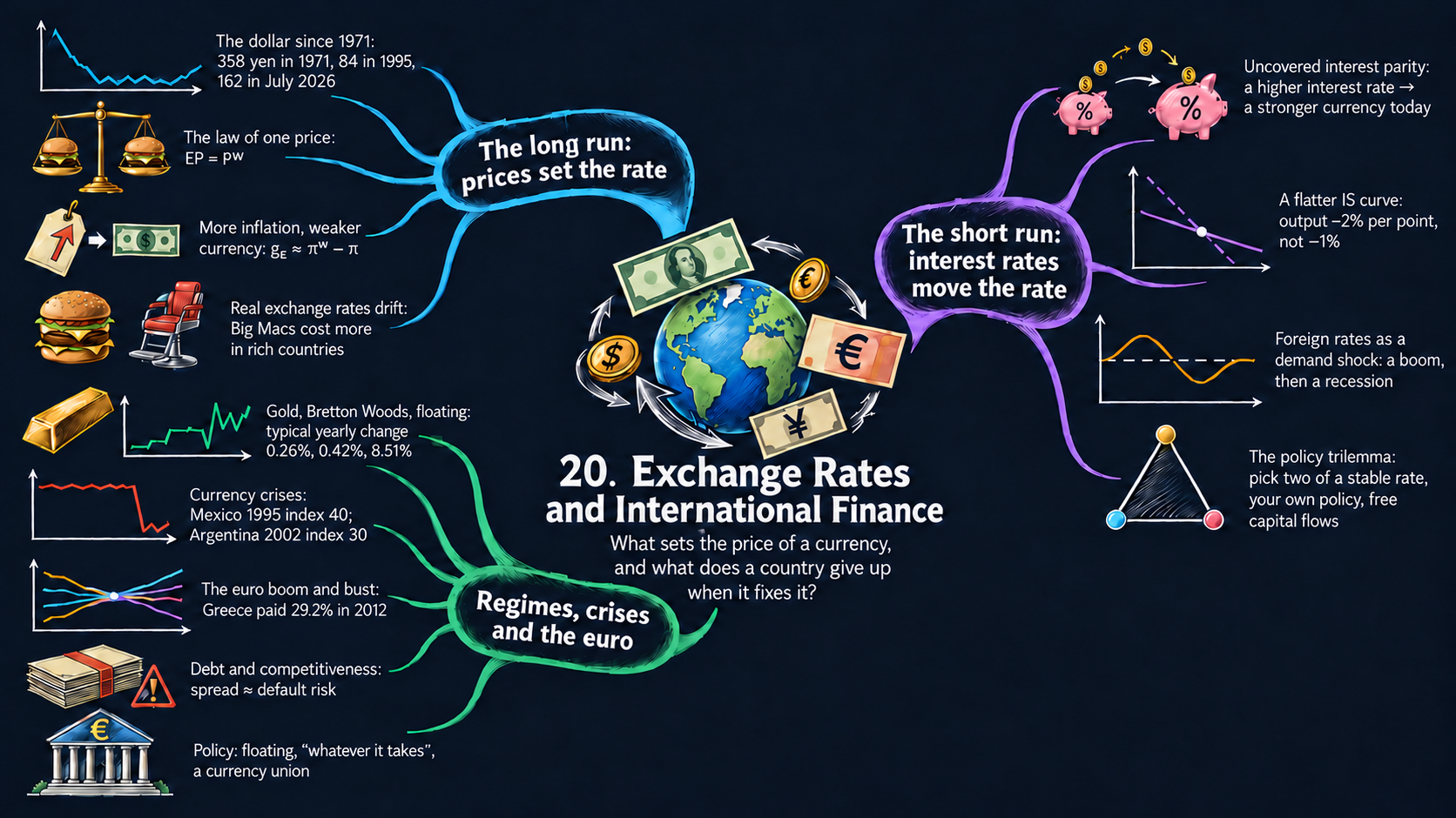
Chapter 19 studied trade between countries. This chapter adds the price at which their currencies trade, the exchange rate, and asks what moves it in the long run and in the short run. By the end of it you will be able to:

tell the nominal exchange rate (the price of a currency) from the real exchange rate (the price of goods), and derive the long-run exchange rate from the law of one price and the quantity theory, in levels and in growth rates (purchasing power parity), and the drift of real exchange rates (Balassa-Samuelson);
derive uncovered interest parity and use it to explain why the exchange rate jumps with interest rates and why a fixed exchange rate ties a country’s interest rate to the rest of the world;
test the law of one price on data: the yen and the dollar since 1971, and the Big Mac index;
derive the open-economy IS curve and the AD curve, read their comparative statics (a flatter IS curve, a rise in foreign interest rates as an aggregate demand shock), and solve the AS/AD dynamics that follow;
explain the policy trilemma and read the history of exchange-rate regimes, currency crises and the euro crisis in the data;
in Python: build price levels from inflation rates with cumprod, plot two vertical scales in one figure, switch views with Plotly buttons, rebase an index, and reshape tables with melt;
go beyond the textbook’s countries: pick any of up to 200 economies from a list (SelectMultiple), filter rows with isin, compare data from the World Bank, the IMF, the OECD and the Penn World Table, and spot gaps, breaks and differences in definitions.

Model overview

Picture Islandia again, with its own money: paper Islandia dollars, which only the Bank of Islandia may print. Mainland, across the water, pays in its own money, which we call the euro (so that the units read as in the book’s examples). Harbor Boatworks sells some of its boats in Mainland, and islanders buy boats and other goods from Mainland, so every deal needs a price at which dollars trade for euros: the exchange rate. What decides that price over decades, and why can it jump overnight when the Bank of Islandia changes its interest rate? We follow Islandia through seven small models to find out.

The big idea

The question. What sets the price of Islandia’s money in terms of Mainland’s money, over decades and from one week to the next, and how does that price feed back into output and inflation at home?

The answer in one sentence. In the long run the exchange rate follows the two price levels (purchasing power parity), while in the short run, with sticky prices, it follows the gap between the two interest rates (uncovered interest parity), and through net exports it flattens the IS curve and turns Mainland’s interest rate into a demand shock for Islandia.

What goes in and what comes out. We choose the money, velocity and output of both countries, the productivity of their sectors, the two interest rates and what investors expect, and the parameters of the short-run model. The model gives back the nominal and real exchange rates and their growth rates, the interest rate a fixed exchange rate requires, and Islandia’s output and inflation after a shock from abroad.

Road map.

Exchange rates in the long run: the law of one price and PPP: the long-run exchange rate, in levels and in growth rates.
Why real exchange rates drift: the Balassa-Samuelson effect: why fast-growing countries look expensive.
Exchange rates in the short run: uncovered interest parity: why the exchange rate jumps with interest rates.
Fixed exchange rates and the policy trilemma: what a peg costs.
The open-economy IS curve: trade joins investment in the short-run model.
The open economy in the AS/AD model: a rise in Mainland’s interest rate, period by period.
The arithmetic of the euro crisis: interest bills, spreads and wages inside a currency union.
Model in code: the key results as Python functions, checked with numbers.

Notation. A bar over a letter marks a parameter, a number set outside the model, such as $\bar{b}_{nx}$; letters without a bar are endogenous variables. As in the book, a bar over a price or an exchange rate, such as $\bar{E}$, marks instead its long-run value. A superscript $w$ (“world”) marks Mainland.

Symbol	Meaning	Type
$E_t$	nominal exchange rate: euros per dollar	endogenous
$P, P^w$	price levels of Islandia (in dollars) and Mainland (in euros)	endogenous
$RER \equiv EP/P^w$	real exchange rate: Mainland goods per Islandia good	endogenous
$\bar{E}, \bar{P}, \overline{RER}$	a bar on a price or an exchange rate marks its long-run value	notation
$\bar{M}, \bar{V}, \bar{Y}$ and $\bar{M}^w, \bar{V}^w, \bar{Y}^w$	money, velocity and output in Islandia and in Mainland	parameters
$\pi, \pi^w$	inflation in Islandia and in Mainland	endogenous
$A_T, A_N, \theta$	productivity in traded and nontraded goods, weight of traded goods in the price level	parameters
$i_t, i^w$	nominal interest rates on Islandia’s and Mainland’s bonds	parameters
$E^e_{t+1}$	the exchange rate investors expect next year	parameter
$R_t$, $NX_t$, $\tilde{Y}_t$	Islandia’s real interest rate, net exports and short-run output	endogenous
$\bar{R}^w, \bar{r}$	Mainland’s real rate; the return on capital, its marginal product	parameters
$\bar{a}, \bar{b}, \bar{a}_{nx}, \bar{b}_{nx}, \bar{m}, \bar{\nu}, \bar{\pi}$	IS, policy-rule and Phillips-curve parameters	parameters
$g_x$, $\Delta x$	the growth rate and the change of $x$	notation

Exchange rates in the long run: the law of one price and PPP

Assumptions

1. The exchange rate. $E$ is the nominal exchange rate: the number of euros that one dollar buys, for example 0.92. It is the price of Islandia’s money. When $E$ goes up, a dollar fetches more euros and the dollar appreciates. When $E$ goes down, the dollar depreciates.

2. Arbitrage in goods. Suppose a fishing net were cheaper in Islandia than in Mainland, once both prices are put in euros. Traders would buy nets in Islandia, ship them across and sell them in Mainland. Their buying lifts the Islandia price and their selling lowers the Mainland price, until the gap closes. In the long run this leaves the law of one price. With $P$ the net’s price in Islandia (in dollars) and $P^w$ its price in Mainland (in euros):

Key result: the law of one price

\[EP = P^w. \tag{1}\]

The left side converts the dollar price into euros: euros per dollar times dollars per net gives euros per net, the unit of the right side. Shipping costs, tariffs and taxes can keep the two sides apart, but only by about the size of those frictions.

Islandia in numbers. At $E = 0.92$, a net that costs 100 dollars in Islandia must cost 92 euros in Mainland.

3. Price levels come from money. Apply equation (1) to the whole basket of goods of each country, so that $P$ and $P^w$ become the two price levels. In the long run each one follows from the quantity theory of money (Chapter 8): $M_tV_t = P_tY_t$, with constant velocity $\bar{V}$ and output at potential $\bar{Y}$. So $\bar{P} = \bar{M}\bar{V}/\bar{Y}$ in Islandia and, in the same way, $\bar{P}^w = \bar{M}^w\bar{V}^w/\bar{Y}^w$ in Mainland.

Solving the model

Step 1: the long-run nominal exchange rate. Once the quantity theory has fixed both price levels, $E$ is the only thing in equation (1) that can still adjust. Dividing both sides by $\bar{P}$ gives $\bar{E} = \bar{P}^w/\bar{P}$.

Step 2: money and the exchange rate. Replace each price level with its quantity-theory value:

\[\bar{E} = \frac{\bar{M}^w\bar{V}^w/\bar{Y}^w}{\bar{M}\bar{V}/\bar{Y}} = \frac{\bar{M}^w}{\bar{M}}\times\frac{\bar{V}^w}{\bar{V}}\times\frac{\bar{Y}}{\bar{Y}^w}.\]

Logs turn the products into sums (Appendix C.4):

\[\ln\bar{E} = (\ln\bar{M}^w - \ln\bar{M}) + (\ln\bar{V}^w - \ln\bar{V}) + (\ln\bar{Y} - \ln\bar{Y}^w).\]

Every coefficient is $+1$ or $-1$, so every elasticity has size one. If the Bank of Islandia doubled the number of dollars, Islandia’s prices would double and each dollar would buy half as many euros. In the long run, the exchange rate is the relative price of two stacks of paper money.

Step 3: pricing goods instead of money. The real exchange rate asks how many Mainland goods one Islandia good is worth:

\[RER \equiv \frac{EP}{P^w}, \qquad \text{in units}\quad \frac{\text{euros}}{\text{dollar}}\times\frac{\text{dollars}}{\text{Islandia good}}\times\frac{\text{Mainland good}}{\text{euros}} = \frac{\text{Mainland goods}}{\text{Islandia good}}.\]

The nominal rate is the price at which two monies trade; the real rate is the price at which two countries’ goods trade. By equation (1), $EP$ and $P^w$ are equal in the long run, so the long-run real exchange rate is $\bar{E}\bar{P}/\bar{P}^w = 1$.

Key result: the long-run exchange rates

\[\bar{E} = \frac{\bar{P}^w}{\bar{P}} \tag{2}\]

\[\overline{RER} = \frac{\bar{E}\bar{P}}{\bar{P}^w} = 1 \tag{3}\]

The two price levels, and so the two money supplies, set the nominal rate; the real rate is pinned at one.

Islandia in numbers. If Islandia’s basket costs 100 dollars and Mainland’s costs 92 euros, $\bar{E} = 92/100 = 0.92$ euros per dollar, and $\overline{RER} = 0.92 \times 100/92 = 1$.

In words

A dollar is worth what it buys. If 100 dollars buy the same basket in Islandia as 92 euros buy in Mainland, then 100 dollars and 92 euros are the same amount of purchasing power, and one dollar is worth 0.92 euros.

Step 4: purchasing power parity in growth rates. Equation (2) is also known as purchasing power parity (PPP). To see how it moves through time, take logs, $\ln\bar{E}_t = \ln\bar{P}^w_t - \ln\bar{P}_t$, and subtract the same equation for the year before. The change in a log is close to a growth rate (Appendix C.5), and the growth rate of a price level is inflation:

\[\underbrace{\ln\bar{E}_t - \ln\bar{E}_{t-1}}_{\approx\, g_E} = \underbrace{(\ln\bar{P}^w_t - \ln\bar{P}^w_{t-1})}_{\approx\,\pi^w} - \underbrace{(\ln\bar{P}_t - \ln\bar{P}_{t-1})}_{\approx\,\pi}.\]

So $g_E \approx \pi^w - \pi$: the growth rule for a ratio, $g_{X/Z} = g_X - g_Z$. The exact yearly version is $\bar{E}_t/\bar{E}_{t-1} = (1+\pi^w)/(1+\pi)$. With the quantity theory and constant velocities, inflation equals money growth minus output growth, $\pi = g_M - g_Y$ (Chapter 8), so the same rule also reads $g_E \approx (g_{M^w} - g_{Y^w}) - (g_M - g_Y)$.

Step 5: the real exchange rate in growth rates. Apply the same log steps to the definition of step 3. A product grows at the sum of the growth rates, and a ratio at their difference, so $g_{RER} \approx g_E + \pi - \pi^w$. When PPP holds, the right side is zero and the real rate stays at one. When the real rate does move, either the nominal rate moved by more than the inflation gap, or prices moved while the nominal rate stood still. Fig. 3 uses this formula to build Japan’s real exchange rate from the data.

Key result: PPP in growth rates

\[g_E \approx \pi^w - \pi \tag{4}\]

\[g_{RER} \approx g_E + \pi - \pi^w \tag{5}\]

The money of the country with faster inflation loses value, at a yearly rate equal to the inflation gap, and that loss leaves the real exchange rate where it was.

Islandia in numbers. If Islandia’s prices rise by 4 percent a year and Mainland’s by 2 percent, the dollar loses about 2 percent a year against the euro. After 25 years it buys $(1.02/1.04)^{25} \approx 0.62$ times as many euros as at the start: about 38 percent fewer.

In words: inflation and the exchange rate

Each year Islandia’s prices outrun Mainland’s, a dollar buys a little less at home compared with what a euro buys in Mainland. The exchange market simply records this: the dollar slides by the inflation gap.

In the long run a currency is worth what it buys, so the country with faster inflation sees its money lose value.

Check your understanding

1. Start from $\bar{E} = 0.92$ euros per dollar. Mainland doubles its money supply, and nothing else changes. What are the new long-run nominal and real exchange rates?

Answer

Mainland’s prices double, so by equation (2) $\bar{E}$ doubles too, to $2 \times 0.92 = 1.84$ euros per dollar: the elasticity of $\bar{E}$ with respect to $\bar{M}^w$ is $+1$ (step 2). The real exchange rate stays at one, by equation (3).

2. Islandia’s inflation falls to 3 percent a year while Mainland’s rises to 5 percent. Does the dollar appreciate or depreciate, and by how much a year? What happens to the real exchange rate?

Answer

By equation (4), $g_E \approx 5 - 3 = 2$ percent a year: the dollar appreciates. By equation (5), $g_{RER} \approx 2 + 3 - 5 = 0$, so the real exchange rate does not change.

What the model predicts

A permanent 1% rise in …	changes $\bar{E}$ (euros per dollar) by	because
Islandia’s money $\bar{M}$	$-1\%$	Islandia’s prices rise 1%
Mainland’s money $\bar{M}^w$	$+1\%$	Mainland’s prices rise 1%
Islandia’s output $\bar{Y}$	$+1\%$	Islandia’s prices fall 1%
Islandia’s velocity $\bar{V}$	$-1\%$	Islandia’s prices rise 1%
any of them	$0$ for $\overline{RER}$	the long-run real exchange rate is always one

Higher inflation, weaker money. For the dollar to lose value against the yen for decades, as in Fig. 1, U.S. inflation must have stayed above Japan’s (equation 4). Fig. 2 puts this to the test.
The level of the nominal rate means nothing by itself. If Islandia swapped 1,000 old dollars for one new dollar, $\bar{E}$ would rise a thousandfold, while the real exchange rate and every real variable would stay put: the classical dichotomy of the long run.
The law holds only roughly. It needs goods that can be shipped. The next block shows how goods that cannot be shipped let real exchange rates drift.

Money moves the nominal exchange rate one for one in the long run, and leaves the real exchange rate at one.

Why real exchange rates drift: the Balassa-Samuelson effect

This block turns the book’s verbal account of the Balassa-Samuelson effect into a small model, with our own notation.

Assumptions

Each country has a traded sector and a nontraded sector. In Islandia, Harbor Boatworks builds boats that sell in Mainland too; the island’s barbers and cafés serve only islanders. Output per worker is $A_T$ in the traded sector and $A_N$ in the nontraded one, and $A^w_T$ and $A^w_N$ in Mainland.
Workers can switch sectors within their own country, so both sectors pay one wage $W$. With competitive firms, the wage equals the value of what a worker makes: $W = P_TA_T = P_NA_N$.
The law of one price, equation (1), holds only for traded goods: $EP_T = P^w_T$.
The price level averages the two prices, with weight $\theta$ on traded goods: $P = P_T^{\theta}P_N^{1-\theta}$, and likewise in Mainland.

Solving the model

Step 1: the price of nontraded goods. Divide $P_TA_T = P_NA_N$ by $A_N$:

\[P_N = P_T\,\frac{A_T}{A_N}.\]

A haircut costs more where the barber could have earned more building boats.

Step 2: the price level. Put $P_N$ into the price level and use the exponent rule $x^{\theta}x^{1-\theta} = x$ (Appendix C.3):

\[P = P_T^{\theta}\left(P_T\frac{A_T}{A_N}\right)^{1-\theta} = P_T^{\theta}P_T^{1-\theta}\left(\frac{A_T}{A_N}\right)^{1-\theta} = P_T\left(\frac{A_T}{A_N}\right)^{1-\theta}.\]

Step 3: the real exchange rate. Write the same expression for Mainland and form $EP/P^w$. The traded-goods factor $EP_T/P^w_T$ equals one by assumption 3, so only the productivity terms survive:

\[RER = \frac{EP_T}{P^w_T}\times\left(\frac{A_T/A_N}{A^w_T/A^w_N}\right)^{1-\theta}.\]

Key result: the Balassa-Samuelson real exchange rate

\[RER = \left(\frac{A_T/A_N}{A^w_T/A^w_N}\right)^{1-\theta} \tag{6}\]

In growth rates, by the rules for powers and ratios, $g_{RER} = (1-\theta)\left[(g_{A_T} - g_{A_N}) - (g_{A^w_T} - g_{A^w_N})\right]$.

Islandia in numbers. With $\theta = 1/2$, if Harbor Boatworks becomes twice as productive while everything else stays the same, $RER = 2^{1/2} \approx 1.41$: Islandia’s goods become about 41 percent dearer than Mainland’s.

In words

Better boatbuilding raises what a worker can earn at Harbor Boatworks, and barbers and cooks must be paid the same to stay. Boats cannot get dearer, because they compete with Mainland’s boats. Haircuts and meals do, because their wage bill grows while their productivity does not. So Islandia’s price level, and with it its real exchange rate, rises.

What the model predicts

Fast-growing economies appreciate in real terms. With $\theta = 1/2$, a country whose traded-sector productivity grows 3 points a year faster than the other’s (relative to services) sees its real exchange rate rise by about $1.5\%$ a year, a factor of $1.015^{24} \approx 1.43$ over 24 years. Japan’s real exchange rate climbed in this way while it caught up, until 1995 (Fig. 3).
Rich countries look expensive. At any moment, rich countries have a high $A_T/A_N$, so their services and their price levels are high. A Big Mac contains the cook’s wage and the restaurant’s rent, so it should cost more in rich countries; the Big Mac section after Fig. 3 tests this.
No money is involved. The effect runs through relative productivities, so it can last for decades while the law of one price holds for every traded good.

Productivity gains in traded goods raise wages everywhere, so services, and the whole price level, become dearer.

Check your understanding

1. For a decade, Harbor Boatworks’ productivity grows 4 points a year faster than that of Islandia’s cafés, while Mainland’s two sectors grow at the same pace. With $\theta = 1/2$, how fast does Islandia’s real exchange rate rise?

Answer

By the growth form of equation (6), $g_{RER} = 0.5 \times (4 - 0) = 2$ percent a year.

2. Does this real appreciation mean that boats now cost more in Islandia than in Mainland?

Answer

No. Assumption 3 keeps $EP_T = P^w_T$: boats still obey equation (1). Islandia’s real exchange rate climbs only because nontraded goods, which cannot be shipped, get dearer in Islandia (equation 6).

Exchange rates in the short run: uncovered interest parity

The book argues in words that a higher interest rate makes a currency stronger. This block writes that argument as an equation, uncovered interest parity (UIP), a standard tool of international finance.

Assumptions

Sticky prices. Over a few weeks or months, $P$ and $P^w$ barely move, as with the sticky inflation of the short-run model.
Free financial flows. Investors can hold Islandia’s bonds, which pay the nominal interest rate $i_t$ in dollars and is set by the Bank of Islandia, or Mainland’s bonds, which pay $i^w$ in euros. They look only at the expected return and ignore risk.
An anchor for the future. Investors expect next year’s exchange rate to be $E^e_{t+1}$. PPP, equation (2), pins down the long run, so we hold this expectation fixed when an interest rate changes.

Solving the model

Step 1: two ways to invest a dollar. Kept in Islandia, one dollar becomes $1 + i_t$ dollars after a year. Sent to Mainland, it is first changed into $E_t$ euros, which grow to $E_t(1+i^w)$, and these are changed back at the expected rate $E^e_{t+1}$, giving $E_t(1+i^w)/E^e_{t+1}$ dollars. If one route paid more, money would pour into it until the two expected returns were equal: $1 + i_t = (1+i^w)\,E_t/E^e_{t+1}$.

Step 2: solve for today’s exchange rate. Multiply both sides by $E^e_{t+1}$ and divide by $1+i^w$:

\[E_t = E^e_{t+1}\times\frac{1+i_t}{1+i^w}.\]

Take logs and use $\ln(1+x) \approx x$ for small $x$ (Appendix C.6): $\ln E_t \approx \ln E^e_{t+1} + (i_t - i^w)$. If the interest gap is expected to last $n$ years before the exchange rate returns to its anchor $E^e_{t+n}$, repeating the step $n$ times gives $E_t = E^e_{t+n}\left[(1+i_t)/(1+i^w)\right]^n$, and in logs $\ln E_t \approx \ln E^e_{t+n} + n\,(i_t - i^w)$.

Key result: uncovered interest parity

\[1 + i_t = (1+i^w)\,\frac{E_t}{E^e_{t+1}} \tag{7}\]

\[\ln E_t \approx \ln E^e_{t+n} + n\,(i_t - i^w) \tag{8}\]

A 1-point rise in Islandia’s interest rate, with $i^w$ and the anchor unchanged, makes the dollar jump today by about $n$ percent. The trilemma model of Fig. 7 uses a jump of 5 percent per point, a gap expected to last about 5 years.

Islandia in numbers. Both rates start at 5 percent and the anchor is 0.92 euros per dollar. The Bank of Islandia raises $i_t$ to 6 percent. If the gap lasts a year, $E_t = 0.92 \times 1.06/1.05 \approx 0.9288$, a jump of about 1 percent. If it lasts five years, $(1.06/1.05)^5 \approx 1.048$: a jump of about 4.8 percent.

Step 3: what happens after the jump. Rearrange equation (7) as $E^e_{t+1}/E_t = (1+i^w)/(1+i_t)$. In logs, the expected growth rate of $E$ is $g^e_E \approx i^w - i_t$. When Islandia’s bonds pay more, the dollar must be expected to lose value from then on, by exactly the interest gap, so that dollars are no better to hold than euros.

In words: jump, then slide

The Bank of Islandia raises its rate, and investors everywhere want dollar bonds. They bid up the dollar until it is so dear that it can only be expected to fall back. That is the only way to have both: the dollar jumps at once, then slides back to its anchor.

Step 4: what sticky prices do to the real rate. With sticky prices, $\pi$ and $\pi^w$ are close to zero over a few weeks, so equation (5) gives $g_{RER} \approx g_E$: every surprise move in $E$ is also a move in the real exchange rate. With sticky inflation, a higher nominal rate $i_t$ also means a higher real rate $R_t = i_t - \pi^e_t$ (the Fisher equation), so the same chain starts from the real interest rate:

\[\uparrow R_t \;\Rightarrow\; \uparrow E_t \;\Rightarrow\; \uparrow \frac{E_tP}{P^w}.\]

What the model predicts

Change	Effect on $E_t$ today	Effect on the real exchange rate
Islandia’s rate $i_t$ up 1 point	up about $n$ percent (dollar appreciates)	up by the same percent
Mainland’s rate $i^w$ up 1 point	down about $n$ percent (dollar depreciates)	down by the same percent
expected future rate $E^e$ up 1%	up 1% (elasticity one)	up 1%

	Long run	Short run
nominal exchange rate $E$	relative price levels, PPP (equation 2)	interest rates and expectations, UIP (equation 8)
real exchange rate $EP/P^w$	equal to one (equation 3)	moves with $E$, because prices are sticky

In the short run the exchange rate follows interest rates: a higher rate at home makes the currency jump up, then slide back.

Check your understanding

1. Mainland’s central bank raises $i^w$ by 1 point, and investors expect the gap to last 3 years. The Bank of Islandia does not move. Roughly what happens to the dollar today?

Answer

By equation (8), $\ln E_t$ changes by about $n\,(i_t - i^w) = 3 \times (-1) = -3$, so the dollar falls by about 3 percent today.

2. After the Bank of Islandia raises its rate, why must investors expect the dollar to depreciate?

Answer

Equation (7) says that both bonds must have the same expected return in dollars. Islandia’s bonds now pay more interest, so the euro route must make up the difference through an expected rise in the euro: $g^e_E \approx i^w - i_t < 0$ (step 3).

Fixed exchange rates and the policy trilemma

Assumptions

The Bank of Islandia promises to trade dollars for euros at a fixed rate $E_{fix}$, and holds foreign exchange reserves, a stock of euros, to keep that promise.
Investors trust the promise, so they expect the rate to stay put: $E^e_{t+1} = E_t = E_{fix}$.
Money flows freely across the water, so uncovered interest parity, equation (7), holds.

Solving the model

Step 1: the interest rate is no longer free. Put $E_t = E^e_{t+1}$ into equation (7). The ratio $E_t/E^e_{t+1}$ becomes one, so $1 + i_t = 1 + i^w$.

Key result: a credible peg ties the interest rate

\[i_t = i^w \tag{9}\]

With a trusted peg and open financial markets, the Bank of Islandia must copy Mainland’s interest rate, whatever is happening on the island.

Islandia in numbers. If Mainland’s rate is 5 percent, so is Islandia’s.

In words

If the dollar paid less interest than the euro while trading at a guaranteed rate, nobody would hold dollars; if it paid more, everybody would. Only an equal rate keeps money still. So once the Bank of Islandia has fixed the price of the dollar, Mainland’s central bank in effect sets Islandia’s interest rate.

Step 2: prices are no longer free either. In the long run, equation (2) with $\bar{E} = E_{fix}$ gives $\bar{P} = \bar{P}^w/E_{fix}$: Islandia’s price level must move one for one with Mainland’s. Equation (4) with $g_E = 0$ gives $\pi = \pi^w$, and by the quantity theory, Islandia’s money growth must match Mainland’s (adjusted for output growth). That is how a peg can import a trusted central bank, and also why it breaks when a government needs to print money to pay its bills (Chapter 8).

Step 3: the gold standard is a law of one price for gold. Under the gold standard each country fixed the price of an ounce of gold in its own money: $P^{gold}$ dollars in the United States, $P^{gold,w}$ pounds in Britain. Apply equation (2) to gold alone: $E = P^{gold,w}/P^{gold}$ pounds per dollar. Fig. 6 computes this gold parity.

Step 4: a peg that markets doubt. Suppose investors start to fear a devaluation and expect $E^e_{t+1}$ below $E_{fix}$. Solve equation (7) for the interest rate:

\[1 + i_t = (1+i^w)\,\frac{E_{fix}}{E^e_{t+1}}, \qquad\text{so}\qquad i_t \approx i^w + \text{expected percent depreciation}.\]

With $i^w = 5$ percent and an expected devaluation of 10 percent, holding dollars requires $i_t = 1.05/0.90 - 1 \approx 16.7$ percent. If the Bank of Islandia stops short of that, investors swap their dollars for its reserves; when the reserves run out, the peg breaks. Mexico in 1994, Asia in 1997 and Argentina in 2002 went through this (Fig. 8).

What the model predicts

UIP ties together three things: the exchange rate, the domestic interest rate, and the freedom of money to cross borders. Fix any two and the third follows. This is the policy trilemma of Fig. 7:

Regime (side of the triangle)	Keeps	Gives up	Why, in equations
floating rate (United States)	monetary autonomy, free flows	a stable exchange rate	$i_t$ is chosen freely, so $E_t$ moves with $i_t - i^w$ (equation 8)
currency board or monetary union (Argentina 1991–2001, the euro)	a stable rate, free flows	monetary autonomy	$E_t$ fixed and UIP hold, so $i_t = i^w$ (equation 9)
capital controls (China 1996–2005)	a stable rate, monetary autonomy	free flows	$i_t \neq i^w$ with $E$ fixed breaks UIP, so trading in the currency must be rationed

Of a fixed exchange rate, free financial flows and its own interest rate, a country can keep any two, never all three.

Check your understanding

1. Islandia pegs to the euro. Mainland’s rate is 3 percent, and markets start to expect the dollar to lose 5 percent. What interest rate must the Bank of Islandia set to keep investors holding dollars?

Answer

By equation (7) with $E_{fix}/E^e_{t+1} = 1/0.95$, $i_t = 1.03/0.95 - 1 \approx 8.4$ percent. The rough rule, $3 + 5 = 8$ percent, is a little too low, because a 5 percent fall is not a very small change.

2. A recession hits Islandia, but not Mainland. Can the Bank of Islandia cut its rate while it keeps both the peg and free financial flows?

Answer

No. With the peg and free flows, equation (9) forces $i_t = i^w$. To cut its rate it must give up one of the two: let the dollar float, or restrict trading in the currency. That is the trilemma.

The open-economy IS curve

Assumptions

Net exports and the real exchange rate. When Islandia’s goods are dear compared with Mainland’s (a high real exchange rate), Harbor Boatworks sells fewer boats abroad and islanders buy more Mainland goods, so net exports $NX \equiv EX - IM$ are low.
The exchange-rate channel. By the UIP block, the real exchange rate rises when Islandia’s real interest rate $R_t$ rises, and falls when Mainland’s real rate $\bar{R}^w$ rises. Together with assumption 1, net exports as a share of potential output fall with the gap between the two real rates, as in the box below. Here $\bar{a}_{nx}$ is the medium-run trade balance and $\bar{b}_{nx} > 0$ measures how strongly trade reacts to the gap. With $\bar{b}_{nx} = 0$ we are back in the closed-economy IS curve of Chapter 11.
The rest of the IS curve is unchanged (Chapter 11): $C_t/\bar{Y}_t = \bar{a}_c$, $G_t/\bar{Y}_t = \bar{a}_g$, $I_t/\bar{Y}_t = \bar{a}_i - \bar{b}_i(R_t - \bar{r})$, where $\bar{r}$ is the marginal product of capital; and all output is spent, $Y_t = C_t + I_t + G_t + NX_t$. Short-run output is $\tilde{Y}_t \equiv (Y_t - \bar{Y}_t)/\bar{Y}_t$.

Key result: net exports

\[\frac{NX_t}{\bar{Y}_t} = \bar{a}_{nx} - \bar{b}_{nx}\,(R_t - \bar{R}^w) \tag{10}\]

A higher real rate in Islandia strengthens the dollar and cuts net exports; a higher real rate in Mainland does the opposite.

Solving the model

Step 1: add and subtract $\bar{r}$. Investment depends on $R_t - \bar{r}$, but net exports on $R_t - \bar{R}^w$. Write $R_t - \bar{R}^w = (R_t - \bar{r}) - (\bar{R}^w - \bar{r})$ and multiply out:

\[\frac{NX_t}{\bar{Y}_t} = \bar{a}_{nx} - \bar{b}_{nx}(R_t - \bar{r}) + \bar{b}_{nx}(\bar{R}^w - \bar{r}).\]

Nothing has really changed, since the two $\bar{r}$ terms cancel. But now trade reacts to the same gap as investment, plus a term that only Mainland can move.

Step 2: divide spending by potential output. Divide $Y_t = C_t + I_t + G_t + NX_t$ by $\bar{Y}_t$ and put in each share:

\[\frac{Y_t}{\bar{Y}_t} = \bar{a}_c + \left[\bar{a}_i - \bar{b}_i(R_t - \bar{r})\right] + \bar{a}_g + \left[\bar{a}_{nx} - \bar{b}_{nx}(R_t - \bar{r}) + \bar{b}_{nx}(\bar{R}^w - \bar{r})\right].\]

Step 3: collect terms. Subtract 1 from both sides, since $\tilde{Y}_t = Y_t/\bar{Y}_t - 1$, and group the constants and the $(R_t - \bar{r})$ terms.

Key result: the open-economy IS curve

\[\tilde{Y}_t = \bar{a} - \bar{b}\,(R_t - \bar{r}), \qquad \bar{a} \equiv \bar{a}_c + \bar{a}_i + \bar{a}_g + \bar{a}_{nx} - 1 + \bar{b}_{nx}(\bar{R}^w - \bar{r}), \qquad \bar{b} \equiv \bar{b}_i + \bar{b}_{nx}. \tag{11}\]

The curve has the same form as in a closed economy, so every tool of the short-run model still works. Only the two parameters mean more: $\bar{b}$ adds the trade channel to the investment channel, and $\bar{a}$ now holds a demand shock from Mainland.

Islandia in numbers. With $\bar{b}_i = 1$ and $\bar{b}_{nx} = 1$, $\bar{b} = 2$. A rise in $R_t$ from $\bar{r} = 5$ to 6 percent lowers output by 2 percent, against 1 percent with no trade channel (Fig. 4).

In words: why trade reacts like investment

Islanders’ saving can build boats at home or be lent to Mainland: $S = I + NX$ (Chapter 19). When the Bank of Islandia raises the real rate, both uses lose at once. Harbor Boatworks invests less because borrowing costs more, and the stronger dollar makes its boats harder to sell abroad.

Step 4: the slope. Solve equation (11) for the interest rate: $R_t - \bar{r} = (\bar{a} - \tilde{Y}_t)/\bar{b}$. With the output gap on the horizontal axis, the IS curve has slope $-1/\bar{b}$, so a larger $\bar{b}$ makes it flatter.

What the model predicts

Change	Effect on $\bar{a}$ or $\bar{b}$	What moves
Islandia’s real rate $R_t$ up 1 point	none	a move along the IS curve: $\tilde{Y}_t$ falls by $\bar{b} = \bar{b}_i + \bar{b}_{nx}$, half of it through trade here
Mainland’s real rate $\bar{R}^w$ up 1 point	$\bar{a}$ rises by $\bar{b}_{nx}$	the IS curve shifts right
a recession in Mainland lowers $\bar{a}_{nx}$	$\bar{a}$ falls by the same amount	the IS curve shifts left
trade more sensitive, $\bar{b}_{nx}$ up	$\bar{b}$ rises	the IS curve gets flatter

In the long run Mainland’s real rate must equal the world marginal product of capital, $\bar{R}^w = \bar{r}$, so the foreign term in $\bar{a}$ drops out and $\bar{a} = 0$ in the long run, as before.

In an open economy the interest rate works through trade as well as investment, so the IS curve is flatter.

Check your understanding

1. With $\bar{b}_i = 1$ and $\bar{b}_{nx} = 1$, Mainland’s real rate rises from 5 to 8 percent, while the Bank of Islandia keeps $R_t = \bar{r} = 5$ percent. How large is Islandia’s demand shock, and what is short-run output?

Answer

By equation (11), $\bar{a}$ rises by $\bar{b}_{nx}(\bar{R}^w - \bar{r}) = 1 \times (8 - 5) = 3$. With $R_t = \bar{r}$, $\tilde{Y}_t = \bar{a} = 3$ percent: a boom driven by a weaker dollar and higher net exports.

2. Islanders’ trade turns less sensitive, $\bar{b}_{nx} = 0.5$. Is the IS curve flatter or steeper, and how much does a 1-point rise in $R_t$ now lower output?

Answer

Now $\bar{b} = 1 + 0.5 = 1.5$, smaller than 2, so the IS curve (slope $-1/\bar{b}$) is steeper. A 1-point rise in $R_t$ lowers output by 1.5 percent instead of 2 (equation 11).

The open economy in the AS/AD model

Assumptions

The open-economy IS curve, equation (11).
The policy rule of Chapter 13: the Bank of Islandia sets the real interest rate above $\bar{r}$ when inflation is above its target, $R_t - \bar{r} = \bar{m}(\pi_t - \bar{\pi})$.
The Phillips curve with adaptive expectations (Chapter 12), read as an AS curve: $\pi_t = \pi_{t-1} + \bar{\nu}\tilde{Y}_t$.

Solving the model

Step 1: the AD curve. Put the policy rule into the IS curve: $\tilde{Y}_t = \bar{a} - \bar{b}(R_t - \bar{r}) = \bar{a} - \bar{b}\bar{m}(\pi_t - \bar{\pi})$.

Step 2: where AD meets AS. Put the AS curve into the AD curve and solve for $\tilde{Y}_t$:

\[\tilde{Y}_t = \bar{a} - \bar{b}\bar{m}(\pi_{t-1} + \bar{\nu}\tilde{Y}_t - \bar{\pi}) \;\Longrightarrow\; \tilde{Y}_t(1 + \bar{b}\bar{m}\bar{\nu}) = \bar{a} - \bar{b}\bar{m}(\pi_{t-1} - \bar{\pi}).\]

Dividing by $1 + \bar{b}\bar{m}\bar{\nu}$ gives output, and the AS curve then gives inflation.

Key result: the open-economy AD curve and the short-run equilibrium

\[\tilde{Y}_t = \bar{a} - \bar{b}\bar{m}\,(\pi_t - \bar{\pi}) \tag{12}\]

\[\tilde{Y}_t = \frac{\bar{a} - \bar{b}\bar{m}(\pi_{t-1} - \bar{\pi})}{1 + \bar{b}\bar{m}\bar{\nu}}, \qquad \pi_t = \pi_{t-1} + \bar{\nu}\tilde{Y}_t \tag{13}\]

The AD curve has slope $-1/(\bar{b}\bar{m})$, so the trade channel, by raising $\bar{b}$, makes it flatter.

Islandia in numbers. With $\bar{b} = 2$, $\bar{m} = 1/2$ and $\bar{\nu} = 1$, $\bar{b}\bar{m} = 1$ and the denominator is 2. Mainland’s real rate 2 points above $\bar{r}$ gives $\bar{a} = 1 \times 2 = 2$, so in the first period $\tilde{Y}_1 = 2/2 = 1$ percent and $\pi_1 = 2 + 1 = 3$ percent.

Step 3: the dynamics. Call $x_t \equiv \pi_t - \bar{\pi}$ the inflation gap. Equation (13) in the AS curve gives $x_t = x_{t-1} + \bar{\nu}\tilde{Y}_t = \left(x_{t-1} + \bar{\nu}\bar{a}\right)/(1 + \bar{b}\bar{m}\bar{\nu})$. While $\bar{a}$ stays constant, this difference equation (Appendix C.10) has the resting point $x^* = \bar{a}/(\bar{b}\bar{m})$, where output is back at potential, and the distance to it shrinks by the same factor every period:

\[x_t - x^* = \frac{x_{t-1} - x^*}{1 + \bar{b}\bar{m}\bar{\nu}}.\]

Step 4: a rise in Mainland’s interest rate. In Fig. 5, Mainland’s real rate sits 2 points above $\bar{r} = 5$ percent in periods 1 to 9. By equation (11) that is a demand shock $\bar{a} = \bar{b}_{nx}(\bar{R}^w - \bar{r}) = 2$ for Islandia. With the numbers in the box:

period 1: $\tilde{Y}_1 = 1$ percent and $\pi_1 = 3$ percent;
periods 2 to 9: the resting point is $x^* = 2/1 = 2$, so inflation heads for 4 percent, and the remaining gap halves each period ($\pi_2 = 3.5$, output $0.5$ percent);
period 10: the shock ends, so $\bar{a} = 0$ and the resting point is back at $x^* = 0$. With $\pi_9 \approx 4$, $\tilde{Y}_{10} = (0 - 1 \times 2)/2 \approx -1$ percent: a recession, after which inflation halves its gap to 2 percent each period.

In words: a shock from across the water

Mainland tightens, investors move toward euros, and the dollar weakens. Harbor Boatworks’ boats become cheap abroad, so Islandia booms and inflation rises. The Bank of Islandia leans against it, and the boom fades. When Mainland’s rate comes back down, the dollar recovers, net exports fall, and the inflation that built up now has to be squeezed out with a recession.

What the model predicts

Monetary policy travels across borders. Tighter money in Mainland weakens the dollar, raises Islandia’s net exports and acts like any positive demand shock: a boom, then higher inflation, then a recession once Mainland’s rate returns to normal. A recession in Mainland pushes the other way, by lowering $\bar{a}_{nx}$, so the net effect of Mainland’s tightening can have either sign.
A larger $\bar{b}$ makes the AD curve flatter. For a given demand shock, output moves less on impact (the denominator $1 + \bar{b}\bar{m}\bar{\nu}$ is larger), because the Bank’s rate moves now work through trade as well as investment.

Shock in period 1	$\tilde{Y}_1$	$\pi_1$	AD curve
$\bar{R}^w$ up 2 points (Fig. 5), $\bar{b} = 2$	$+1$	3	shifts right by $\bar{b}_{nx} \times 2 = 2$
the same shock with $\bar{b}_{nx} = 0$	0	2	does not move: no trade channel
a 1-point cut in $\bar{a}_{nx}$ (recession abroad)	$-0.5$	1.5	shifts left by 1

A rise in foreign interest rates is a demand shock at home: first a boom, then inflation, then a recession when it ends.

Check your understanding

1. Mainland’s real rate rises by only 1 point above $\bar{r}$, with the baseline $\bar{b}_i = \bar{b}_{nx} = 1$, $\bar{m} = 1/2$, $\bar{\nu} = 1$ and $\bar{\pi} = 2$ percent. What are output and inflation in the first period?

Answer

Now $\bar{a} = 1 \times 1 = 1$. Equation (13) with $\pi_0 = \bar{\pi}$ gives $\tilde{Y}_1 = 1/2 = 0.5$ percent, and $\pi_1 = 2 + 0.5 = 2.5$ percent.

2. In the long run, where do Islandia’s output and inflation settle while Mainland’s rate stays high, and why?

Answer

Output returns to potential and inflation settles at $\bar{\pi} + x^* = 2 + 2 = 4$ percent (step 3). At that inflation rate the Bank’s higher real rate exactly offsets the boost from Mainland, so the AD curve gives $\tilde{Y} = 0$ (equation 12).

The arithmetic of the euro crisis

The euro section of the chapter has no formal model, but three short pieces of arithmetic sit behind its figures. To tell them as a story, suppose Islandia gives up its dollar and shares Mainland’s euro, and the Islandia Treasury borrows by selling bonds to islanders and to lenders on Mainland.

Definitions

Sovereign debt $D$ is the government’s debt; $D/Y$ is the debt-GDP ratio, and $i$ is the nominal interest rate the government pays on it.
A bond’s default probability $p$ is the chance that the government does not repay it.
The unit labor cost is the wage cost of one unit of output: the nominal wage $W$ divided by real output per worker $Y/L$, $ULC \equiv W/(Y/L)$.

Solving the model

Step 1: the interest bill. The Treasury pays $i \times D$ in interest each year. Divide by $Y$: interest in percent of GDP is $i \times (D/Y)$. With debt equal to 100 percent of GDP, each point on the interest rate costs one point of GDP a year: a rate that climbs from 2 to 6 percent lifts the bill from 2 to 6 percent of GDP.

Step 2: why yields converged and then split (Fig. 9). A lender who cares only about the expected return must earn as much on a risky bond as on a safe one, the Mainland bond with rate $i^{safe}$. If the Treasury’s bond pays $1 + i$ with probability $1 - p$ and nothing otherwise, then $(1 - p)(1 + i) = 1 + i^{safe}$. Solve for $i$, and use the approximation of Appendix C.6 for small $p$ and $i$.

Step 3: competitiveness in a currency union (Fig. 13). The unit labor cost is a ratio, so by the growth rule for a ratio its growth rate is wage growth minus productivity growth.

Key result: spreads and unit labor costs

\[i = \frac{1 + i^{safe}}{1 - p} - 1 \;\approx\; i^{safe} + p \tag{14}\]

\[g_{ULC} = g_W - g_{Y/L} \tag{15}\]

The spread over the safe bond is roughly the default probability.

Islandia in numbers. With a safe rate of 2 percent and a default probability of 3 percent, the Treasury pays $1.02/0.97 - 1 \approx 5.15$ percent, a spread of about 3 points. If Islandia’s wages grow 4 percent a year and its productivity 1 percent, while both grow 1.5 percent in Mainland, Islandia’s real exchange rate rises by about 3 percent a year: $1.03^{10} \approx 1.34$ over a decade.

Before the euro, spreads also held the expected inflation gap (by the Fisher equation, $i = R + \pi^e$). One currency removed that part, so yields converged; after 2008, fear of default opened the spreads again. Inside the union the nominal exchange rate between Islandia and Mainland is fixed at one, so their real exchange rate is the ratio of their price levels. If firms set prices as a fixed markup over unit labor cost, equation (5) with $g_E = 0$ gives $g_{RER} = g_{ULC} - g^w_{ULC}$, the gap between the two growth rates of equation (15).

In words

Sharing Mainland’s money takes away the inflation premium, so Islandia borrows cheaply at first. But it also takes away the exchange rate as a shock absorber. If islanders’ wages race ahead of their productivity, Harbor Boatworks’ boats get dearer abroad, and there is no dollar left to fall and set prices right.

What the model predicts

Crises can feed themselves. At high debt, a rise in the feared default probability $p$ raises $i$ by equation (14), which raises the interest bill, which makes default more likely. Investors’ fears can come true because they hold them. A central bank that promises to buy the bonds lowers $p$ and can stop the spiral.
No exchange rate to fall back on. A country with its own money can win back competitiveness by letting $E$ fall. Inside a monetary union $g_E = 0$, so the real exchange rate can fall only if wages grow more slowly than productivity at home (equation 15), or faster abroad. That is slow and painful, and it helps explain the high unemployment of southern Europe.

Inside a currency union, competitiveness can be regained only through wages and productivity, which is slow and painful.

Check your understanding

1. The Treasury’s debt is 100 percent of GDP. Investors’ feared default probability rises from 1 to 4 percent, with a safe rate of 2 percent. Using the approximation in equation (14), by how much does the yearly interest bill rise, in percent of GDP?

Answer

By equation (14) the rate rises from about $2 + 1 = 3$ to $2 + 4 = 6$ percent. At a debt of 100 percent of GDP the bill is $i \times D/Y$, so it rises from 3 to 6 percent of GDP: 3 points more each year (step 1).

2. In the union, Islandia’s wages grow 2 percent a year and its productivity 2 percent, while in Mainland wages grow 3 percent and productivity 1 percent. Does Islandia gain or lose competitiveness?

Answer

By equation (15), $g_{ULC} = 2 - 2 = 0$ in Islandia and $3 - 1 = 2$ percent in Mainland. Islandia’s real exchange rate falls by about 2 percent a year: its goods get cheaper relative to Mainland’s, so it gains competitiveness.

Recap

In the long run, PPP: the exchange rate equals the ratio of the price levels, $\bar{E} = \bar{P}^w/\bar{P}$, and the money with faster inflation loses value, $g_E \approx \pi^w - \pi$ (Fig. 1 and Fig. 2).
Real exchange rates drift when traded-goods productivity grows faster in one country, the Balassa-Samuelson effect (Fig. 3).
In the short run, UIP: with sticky prices, a higher interest rate at home makes the currency, and the real exchange rate, jump up.
The trilemma: a credible peg with free flows forces $i_t = i^w$, so a country keeps only two of three goals (Fig. 7, Fig. 8).
The open-economy IS and AD curves are flatter, $\bar{b} = \bar{b}_i + \bar{b}_{nx}$, and a rise in foreign interest rates is a demand shock at home (Fig. 4 and Fig. 5).
Inside a currency union, spreads track default risk, $i \approx i^{safe} + p$, and competitiveness moves with unit labor costs (Fig. 9, Fig. 13).

Model in code

Now we turn the Key results into Python. The section has four parts: the setup (folded, because it is the same in every chapter), the model as functions, numerical checks of the Key results, and the drawing and data tools that the figures use (folded too). Run its cells once, in order. Every later section of the notebook reuses them.

Setup

Run the setup cells once, before anything else. They load the Python libraries, give every chart the same look, store the address of the chapter’s data and define the helpers that only the book website needs. You can use the notebook without reading them; open the box if you are curious.

Show the setup code

The first cell loads the libraries and sets the look of the charts. Its comments explain each step.

# @title Setup: libraries, chart colors and the data location
# Text after a "#" is a comment: Python ignores it, it is there for human readers.

# Step 1: load the libraries. `import` loads a library, a toolbox written by
# other people, and `as np` gives it a short nickname, so the code stays short.
import numpy as np                              # numbers and arrays
import pandas as pd                             # data tables
import plotly.express as px                     # quick charts from data tables
import plotly.graph_objects as go               # charts built piece by piece
import plotly.io as pio                         # settings shared by every chart
# sliders, buttons and lists for the interactive figures
from ipywidgets import interact, FloatSlider, IntSlider, ToggleButtons, Dropdown, SelectMultiple, fixed

# Step 2: one light blue/green look for every chart
BLUE, TEAL, GREEN, GRAY = "#16528c", "#008070", "#7fb23a", "#8a96a3"
pio.templates.default = "plotly_white"
# the same chart size in Colab and on the website
pio.templates["plotly_white"].layout.update(width=860, height=480)
px.defaults.color_discrete_sequence = [BLUE, TEAL, GREEN, "#5aa0d8", "#0b4f47"]
WIDE = {"description_width": "initial"}         # show the full slider labels

# Step 3, Colab only: let Plotly charts appear inside the interactive widgets.
# `try` runs the indented lines; if the import fails (we are not in Colab),
# `except` skips them.
try:
    import google.colab
    google.colab.output.enable_custom_widget_manager()
except ImportError:
    pass                                        # not running in Colab: nothing to do

# Step 4: the data files of this chapter live in the book's GitHub repository
DATA_URL = "https://raw.githubusercontent.com/quarcs-lab/macro102-site/main/data/ch20/"

The website cannot run Python, so each interactive figure also gets a version with a precomputed slider. The next helper builds those versions. Run it and move on.

# @title Helper for the website versions (run this cell; you do not need to read it)
def slider_figure(make_figure, name, values, start, label=None):
    """Join precomputed versions of a figure with one slider (the website cannot run Python).

    Arguments
        make_figure : the function that draws the figure, e.g. the one of Fig. 4
        name        : the argument the slider moves, e.g. "b_nx"
        values      : the values of that argument to precompute
        start       : the value shown first
        label       : the slider's label (the argument name if None)
    Returns
        one Plotly figure with all versions and a slider that shows one at a time
    """
    # Step 1: draw the figure once for every value
    figures = [make_figure(**{name: v}) for v in values]
    first = values.index(start)
    # Step 2: copy every curve into one figure; only the start value's are visible
    fig = go.Figure(layout=figures[first].layout)
    owner = []                          # which precomputed figure each trace is from
    for i, f in enumerate(figures):
        for trace in f.data:
            trace.visible = (i == first)
            fig.add_trace(trace)
            owner.append(i)
    # Step 3: one slider step per value: its curves, title, labels and shapes
    steps = []
    for i, f in enumerate(figures):
        layout = {"title": f.layout.title.to_plotly_json(),
                  "annotations": [a.to_plotly_json() for a in f.layout.annotations],
                  "shapes": [s.to_plotly_json() for s in f.layout.shapes]}
        visible = [o == i for o in owner]
        steps.append(dict(method="update", label=str(values[i]), args=[{"visible": visible}, layout]))
    fig.update_layout(sliders=[dict(active=first, steps=steps, pad=dict(t=60),
                                    currentvalue=dict(prefix=(label or name) + " = "))])
    return fig

The data figures can show many countries. On the website they use the helpers below: a legend you can click, a slider that changes the data of every line at once, and a menu of country groups.

# @title Helpers for the many-country website versions (run this cell; you do not need to read it)
def compact(y):
    """Round to 4 significant digits, so that the saved figure stays small.

    Arguments
        y : the values of one line (None or NaN for a gap)
    Returns
        the rounded values as a list, with None for every gap
    """
    # `v != v` is True only for NaN, the code for a missing value
    return [None if v is None or v != v else float(f"{v:.4g}") for v in y]


def slim(trace):
    """Make a line smaller: rounded y values, and one hover label for the whole line.

    The hover label comes from the trace name instead of one text per point.

    Arguments
        trace : one line of a Plotly figure
    Returns
        the same line, smaller
    """
    # Step 1: round the y values
    trace.y = compact(trace.y)
    # Step 2: if each point's hover text is just the line's name, use the name once
    if trace.hovertext is not None and len(trace.hovertext) > 0 and trace.hovertext[0] == trace.name:
        trace.hovertext = None
        trace.hovertemplate = trace.hovertemplate.replace("%{hovertext}", "%{fullData.name}")
    return trace


def legend_only(fig, keep):
    """Show the traces named in keep; list the others in the legend only, so a click adds them.

    Arguments
        fig  : a Plotly figure with one trace per country
        keep : the names of the traces drawn at the start
    Returns
        the same figure, with smaller traces
    """
    for trace in fig.data:
        # drawn, or "legendonly": listed in the legend, a click away
        trace.visible = True if trace.name in keep else "legendonly"
        slim(trace)
    return fig


def data_slider(make_figure, name, values, start, title, label=None, **fixed):
    """A slider whose steps replace the y data of every line, so that legend clicks are kept.

    Lines are matched by name, and lines missing at the start value are added empty.

    Arguments
        make_figure : the function that draws the figure
        name        : the argument the slider moves, e.g. "base"
        values      : the values of that argument to precompute
        start       : the value shown first
        title       : the title, a text with {} where the slider value goes
        label       : the slider's label (the argument name if None)
        fixed       : further arguments, passed to make_figure unchanged
    Returns
        one Plotly figure with a slider
    """
    # Step 1: draw the figure once for every value
    figures = {v: make_figure(**{name: v}, **fixed) for v in values}
    fig = go.Figure(layout=figures[start].layout)
    # Step 2: one line per name; a line missing at the start value is added empty
    for v in [start] + list(values):
        for t in figures[v].data:
            if t.name not in [u.name for u in fig.data]:
                t.y = t.y if v == start else [None] * len(t.y)
                fig.add_trace(slim(t))
    # Step 3: one slider step per value: the new y data of every line, the new title
    steps = []
    for v in values:
        ys = {t.name: compact(t.y) for t in figures[v].data}
        new_y = [ys.get(t.name, [None] * len(t.y)) for t in fig.data]
        steps.append(dict(method="update", label=str(v),
                          args=[{"y": new_y}, {"title.text": title.format(v)}]))
    fig.update_layout(title=title.format(start), sliders=[dict(
        active=values.index(start), steps=steps, pad=dict(t=60), currentvalue=dict(prefix=(label or name) + " = "))])
    return fig

# @title Helper: groups of countries for the website menus (run this cell; you do not need to read it)
# Step 1: two groups of countries that the data files do not list
G7 = ["Canada", "France", "Germany", "Italy", "Japan", "United Kingdom", "United States"]
EMERGING = ["Argentina", "Brazil", "China", "India", "Indonesia", "Mexico", "Russia", "Saudi Arabia",
            "South Africa", "Türkiye"]


def country_groups(names, book, book_label, regions=True):
    """The groups of the website menus, for the countries that have data.

    The groups are the textbook's countries, the G7, the euro area, the large emerging economies
    and the World Bank regions. It uses `country_info`, read in the drawing and data tools.

    Arguments
        names      : the countries that have data
        book       : the textbook's countries
        book_label : the menu's name for them, e.g. "Textbook: Japan"
        regions    : True to add one group per World Bank region
    Returns
        a dictionary {group name: list of countries}, without empty groups
    """
    # Step 2: the countries with data, and the euro members among them
    info = country_info[country_info.country.isin(names)]
    euro = list(info[info.euro_since.notna() | (info.country == "Euro area")].country)
    groups = {book_label: list(book), "G7": [c for c in G7 if c in set(names)], "Euro area": euro,
              "Large emerging economies": [c for c in EMERGING if c in set(names)]}
    # Step 3: one group per World Bank region
    if regions:
        for region in sorted(info.region.unique()):
            if region != "Euro area":
                groups[region] = list(info[info.region == region].country)
    # leave out the empty groups
    return {k: v for k, v in groups.items() if v}

# @title Helper: a figure with a menu of country groups (run this cell; you do not need to read it)
def menu_figure(make_figure, options, categories=False):
    """Precompute make_figure for every menu option and join the figures with a dropdown menu.

    With categories=True (bar charts) each option also sets the order and the range of the x-axis.

    Arguments
        make_figure : the function that draws the figure
        options     : maps each menu label to a list of countries, or to a dict of keyword arguments
        categories  : True for bar charts, with one bar per country
    Returns
        one Plotly figure with all versions and a menu that shows one at a time
    """
    # Step 1: draw the figure once for every menu option
    labels = list(options)
    figures = [make_figure(**options[g]) if isinstance(options[g], dict) else make_figure(tuple(options[g]))
               for g in labels]
    # Step 2: copy every line into one figure; only the first option's are visible
    fig = go.Figure(layout=figures[0].layout)
    owner = []                          # which precomputed figure each trace is from
    for i, f in enumerate(figures):
        for trace in f.data:
            trace.visible = (i == 0)
            fig.add_trace(slim(trace))
            owner.append(i)
    # Step 3: one menu button per option: its lines, title, axes, shapes and notes
    buttons = []
    for i, f in enumerate(figures):
        layout = {"title.text": f.layout.title.text, "yaxis.type": f.layout.yaxis.type or "linear",
                  "yaxis.range": f.layout.yaxis.range, "yaxis.tickvals": f.layout.yaxis.tickvals,
                  "yaxis.autorange": f.layout.yaxis.range is None,
                  "shapes": [s.to_plotly_json() for s in f.layout.shapes],
                  "annotations": [a.to_plotly_json() for a in f.layout.annotations]}
        # a bar chart also gets the order of its bars and the range of its x-axis
        if categories:
            names = list(dict.fromkeys(x for t in f.data for x in t.x))
            layout.update({"xaxis.categoryorder": "array", "xaxis.categoryarray": names,
                           "xaxis.range": [-0.5, len(names) - 0.5]})
            # the first option is the one shown at the start
            if i == 0:
                fig.update_xaxes(categoryorder="array", categoryarray=names, range=[-0.5, len(names) - 0.5])
        buttons.append(dict(label=labels[i], method="update",
                            args=[{"visible": [o == i for o in owner]}, layout]))
    # Step 4: the menu sits above the plot, at the left
    fig.update_layout(margin=dict(t=110), updatemenus=[dict(buttons=buttons, active=0, x=0, y=1.02,
                                                            xanchor="left", yanchor="bottom")])
    return fig

The model as functions

Now the Key results become Python functions. Each function’s description names the equation it computes. In the code, Islandia plays the part of the book’s United States and Mainland that of the rest of the world.

One baseline for every diagram. The textbook draws its diagrams without numbers. Both model diagrams of this notebook start from one illustrative set of parameters, which the worked numbers above also use:

marginal product of capital $\bar{r} = 5$ percent, as in Chapter 11’s example, and no demand shock at home, $\bar{a}_c + \bar{a}_i + \bar{a}_g + \bar{a}_{nx} = 1$;
interest sensitivities $\bar{b}_i = 1$ and $\bar{b}_{nx} = 1$, so the total $\bar{b} = 2$ is the value of Chapters 11 and 13, split half and half between investment and trade;
inflation target $\bar{\pi} = 2$ percent, policy response $\bar{m} = 1/2$ and Phillips-curve slope $\bar{\nu} = 1$, as in Chapter 13;
the foreign shock of Fig. 5: the foreign real interest rate is 2 points above $\bar{r}$, at 7 percent, in periods 1 to 9 and back at $\bar{r}$ afterwards.

The first cell stores this baseline. Then it writes the first pieces of the model as functions: the long-run exchange rate, equation (2), the real exchange rate, equation (3), net exports, equation (10), and the part of the demand shock that comes from abroad.

# Step 1: the baseline. Names in capital letters, such as `R_BAR`, are constants:
# we set them once and never change them.
# marginal product of capital r-bar (%), interest sensitivities b_i and b_nx
R_BAR, B_I, B_NX = 5.0, 1.0, 1.0
# inflation target pi-bar (%), policy response m-bar, Phillips-curve slope nu-bar
PI_BAR, M_BAR, NU_BAR = 2.0, 0.5, 1.0
# the foreign rate minus r-bar in periods 1 to A_LAST; T_MAX periods are simulated
RW_GAP, A_LAST, T_MAX = 2.0, 9, 20


# Step 2: the functions. `def` creates a function, a named recipe: its inputs
# are the arguments in parentheses, and `return` gives back the result.
def long_run_exchange_rate(P_w, P):
    """The long-run nominal exchange rate, E-bar.

    Equation (2):  E = P_w / P   (foreign currency per dollar)

    Arguments
        P_w : the foreign price level (Mainland's), in foreign currency per basket
        P   : the U.S. price level (Islandia's), in dollars per basket
    Returns
        the long-run exchange rate E, in foreign currency per dollar
    """
    # the exchange rate at which a basket costs the same in both countries
    return P_w / P


def real_exchange_rate(E, P, P_w):
    """The real exchange rate: the foreign goods needed to buy one U.S. good.

    Equation (3):  RER = E P / P_w

    Arguments
        E   : the nominal exchange rate, foreign currency per dollar
        P   : the U.S. price level, in dollars
        P_w : the foreign price level, in foreign currency
    Returns
        the real exchange rate, RER (1 when the law of one price holds)
    """
    return E * P / P_w


# `R_w=R_BAR` gives an argument a default value, used whenever we do not pass one;
# `b_nx=B_NX` does the same for the interest sensitivity of net exports.
def net_exports(R, R_w=R_BAR, a_nx=0.0, b_nx=B_NX):
    """Net exports, in percent of potential output.

    Equation (10):  NX/Y = a_nx - b_nx (R - R_w)

    Arguments
        R    : the U.S. real interest rate (%)
        R_w  : the foreign real interest rate, R-bar^w (%), r-bar unless we pass another value
        a_nx : the net-exports shock, a-bar_nx (% of potential output)
        b_nx : the interest sensitivity of net exports, b-bar_nx
    Returns
        net exports NX/Y, in percent of potential output
    """
    # a higher U.S. rate than abroad makes the dollar dearer and lowers net exports
    return a_nx - b_nx * (R - R_w)


def foreign_shock(R_w, b_nx=B_NX, r_bar=R_BAR):
    """The part of the demand shock a-bar that comes from abroad.

    Equation (11), its foreign term:  b_nx (R_w - r_bar)

    Arguments
        R_w   : the foreign real interest rate (%)
        b_nx  : the interest sensitivity of net exports, b-bar_nx
        r_bar : the marginal product of capital, r-bar (%)
    Returns
        the shock to a-bar, in percent of potential output
    """
    return b_nx * (R_w - r_bar)

The next four functions are the short-run model: the open-economy IS curve, equation (11), the AD and AS curves, and the point where they cross, equation (13).

def is_curve(R, a=0.0, b_i=B_I, b_nx=B_NX, r_bar=R_BAR):
    """The open-economy IS curve: short-run output for a given real interest rate.

    Equation (11):  Y~ = a - (b_i + b_nx) (R - r_bar), in percent

    Arguments
        R     : the U.S. real interest rate (%)
        a     : the demand shock, a-bar (0 in the baseline)
        b_i   : the interest sensitivity of investment, b-bar_i
        b_nx  : the interest sensitivity of net exports, b-bar_nx
        r_bar : the marginal product of capital, r-bar (%)
    Returns
        short-run output Y~, in percent
    """
    # trade adds b_nx to the slope, so the open-economy IS curve is flatter
    return a - (b_i + b_nx) * (R - r_bar)


def ad_output(pi, a=0.0, m=M_BAR, b=B_I + B_NX):
    """The AD curve with the open-economy b: short-run output for a given inflation rate.

    Equation (12):  Y~ = a - b m (pi - pi_bar)

    Arguments
        pi : inflation (%)
        a  : the demand shock, a-bar
        m  : the policy response, m-bar
        b  : the interest sensitivity of spending, b-bar = b_i + b_nx
    Returns
        short-run output Y~, in percent
    """
    return a - b * m * (pi - PI_BAR)


def as_inflation(Y, pi_e, nu=NU_BAR):
    """The AS curve of Chapter 13: inflation for a given short-run output.

    Equation (13), second part:  pi = pi_e + nu Y~

    Arguments
        Y    : short-run output Y~ (%)
        pi_e : expected inflation, last period's inflation (%)
        nu   : the Phillips-curve slope, nu-bar
    Returns
        inflation pi (%)
    """
    return pi_e + nu * Y


def solve_asad(pi_e, a=0.0, m=M_BAR, b=B_I + B_NX, nu=NU_BAR):
    """Short-run output and inflation in one period, where the AD and AS curves cross.

    Equation (13):  Y~ = (a - b m (pi_e - pi_bar)) / (1 + b m nu),  pi = pi_e + nu Y~

    Arguments
        pi_e : expected inflation, last period's inflation (%)
        a    : the demand shock, a-bar
        m    : the policy response, m-bar
        b    : the interest sensitivity of spending, b-bar = b_i + b_nx
        nu   : the Phillips-curve slope, nu-bar
    Returns
        two numbers: short-run output Y~ and inflation pi
    """
    # Step 1: output where the two curves cross
    Y = (a - b * m * (pi_e - PI_BAR)) / (1 + b * m * nu)
    # Step 2: inflation from the AS curve; `return Y, ...` gives back two results
    return Y, as_inflation(Y, pi_e, nu)

Two more functions take the long-run model one step further. The quantity theory gives each country’s price level, and bs_price_level builds a price level from the prices of traded and nontraded goods, the starting point of equation (6).

def quantity_price(M, V, Y):
    """The long-run price level of the quantity theory, which leads to equation (2).

    The quantity theory:  P = M V / Y

    Arguments
        M : the money supply, M-bar
        V : the velocity of money, V-bar
        Y : real output, Y-bar
    Returns
        the price level P
    """
    return M * V / Y


def bs_price_level(P_T, A_T, A_N, theta=0.5):
    """The price level of the Balassa-Samuelson model, behind equation (6).

    P = P_T^theta P_N^(1-theta), with P_N from equal wages: P_T A_T = P_N A_N

    Arguments
        P_T   : the price of traded goods
        A_T   : productivity in traded goods
        A_N   : productivity in nontraded goods
        theta : the weight of traded goods in the price level
    Returns
        the price level P
    """
    # Step 1: a worker's output in the traded sector is worth P_T A_T: the wage
    wage = P_T * A_T
    # Step 2: the same wage is paid in the nontraded sector
    P_N = wage / A_N
    # Step 3: the price level weights traded and nontraded prices by theta and 1 - theta
    return P_T ** theta * P_N ** (1 - theta)

Uncovered interest parity, equation (7), gives today’s exchange rate from the expected one and the two interest rates. Solved for the interest rate instead, it gives the rate that defends a peg.

def uip_exchange_rate(E_anchor, i, i_w, years=1):
    """Today's exchange rate from uncovered interest parity.

    Equation (7), applied `years` times:  E = E_anchor ((1 + i) / (1 + i_w))^years

    Arguments
        E_anchor : the exchange rate investors expect at the end, E^e
        i, i_w   : the U.S. and the foreign interest rate (%)
        years    : how many years the gap between them lasts
    Returns
        today's exchange rate E
    """
    # the rates are in percent, so i / 100 is the rate as a share
    return E_anchor * ((1 + i / 100) / (1 + i_w / 100)) ** years


def defend_peg_rate(i_w, expected_fall):
    """The interest rate that keeps uncovered interest parity when the peg may fall.

    Equation (7), solved for i, with E fixed today and expected to fall by `expected_fall` %

    Arguments
        i_w           : the foreign interest rate (%)
        expected_fall : the devaluation markets expect (%)
    Returns
        the interest rate i that defends the peg (%)
    """
    E_ratio = 1 / (1 - expected_fall / 100)              # E_fix / E_expected
    # equation (7): 1 + i = (1 + i_w) E_fix / E_expected
    return 100 * ((1 + i_w / 100) * E_ratio - 1)

Fig. 5 follows the economy period by period. Each period, firms expect last period’s inflation, and the economy jumps to the point where that period’s AD and AS curves cross. simulate repeats this step; shock_list builds the list of demand shocks, one value per period.

def shock_list(size, last=A_LAST):
    """The demand shocks of Fig. 5, one value per period.

    The shock has the given size in periods 1, ..., last and is zero afterwards, for T_MAX periods.

    Arguments
        size : the size of the shock, a-bar
        last : the last period of the shock
    Returns
        a list of T_MAX shocks
    """
    # `values = []` starts an empty list, and `values.append(x)` adds x at its end.
    # `for t in range(1, T_MAX + 1)` repeats the indented lines for t = 1, ..., 20.
    values = []
    for t in range(1, T_MAX + 1):
        if t <= last:
            values.append(size)
        else:
            values.append(0.0)
    return values


def simulate(a_list, m=M_BAR, b=B_I + B_NX, nu=NU_BAR):
    """The AS/AD model, solved period by period.

    Equation (13) in every period; period 0 is the steady state (Y~ = 0, pi = pi_bar).

    Arguments
        a_list : the demand shock of each period (from shock_list)
        m      : the policy response, m-bar
        b      : the interest sensitivity of spending, b-bar = b_i + b_nx
        nu     : the Phillips-curve slope, nu-bar
    Returns
        a table with one row per period: the shock, expected inflation, output and inflation
    """
    # Step 1: period 0. `dict(period=0, Y=0.0)` is a dictionary, a set of named
    # values, and `rows` is a list of them, one per period.
    rows = [dict(period=0, a=0.0, pi_e=PI_BAR, Y=0.0, pi=PI_BAR)]
    # Step 2: each period, solve equation (13)
    for t in range(1, len(a_list) + 1):
        # adaptive expectations: `rows[-1]["pi"]` is the value named "pi" in the
        # last element of the list, last period's inflation
        pi_e = rows[-1]["pi"]
        Y, pi = solve_asad(pi_e, a_list[t - 1], m, b, nu)
        rows.append(dict(period=t, a=a_list[t - 1], pi_e=pi_e, Y=Y, pi=pi))
    # Step 3: `pd.DataFrame(rows)` turns the list of dictionaries into a table,
    # one row per dictionary
    return pd.DataFrame(rows)

Checking the key results

The formulas came from algebra. Now we check them with numbers, one Key result at a time. First we try the functions on a few textbook cases.

# Step 1: the law of one price. A chip costs 92 euros in Germany and 100 dollars
# in the U.S.
E = long_run_exchange_rate(P_w=92.0, P=100.0)
# An f-string, f"... {E:.2f}", puts a value into the text; ":.2f" means
# "two decimals", and ":+.1f" also shows the sign.
print(f"Law of one price: E = {E:.2f} euros per dollar")
print(f"Real exchange rate at that E: {real_exchange_rate(E, 100.0, 92.0):.2f}; at E = 1.00: "
      f"{real_exchange_rate(1.0, 100.0, 92.0):.2f}")
# Step 2: net exports and the IS curve when R rises from 5% to 6%
print(f"Net exports when R rises from 5% to 6%: {net_exports(6.0):+.1f}% of potential output")
print(f"IS curve at R = 6%: Y~ = {is_curve(6.0):+.1f}% (without the trade channel: {is_curve(6.0, b_nx=0.0):+.1f}%)")
# Step 3: a foreign rate 2 points above r-bar is a demand shock at home.
# `Y, pi = solve_asad(...)` unpacks the two results into two variables.
a = foreign_shock(R_BAR + RW_GAP)
Y, pi = solve_asad(PI_BAR, a)
print(f"Foreign rate 2 points above r_bar: a = {a:.1f}; first period Y~ = {Y:+.2f}%, inflation = {pi:.2f}%")

Law of one price: E = 0.92 euros per dollar
Real exchange rate at that E: 1.00; at E = 1.00: 1.09
Net exports when R rises from 5% to 6%: -1.0% of potential output
IS curve at R = 6%: Y~ = -2.0% (without the trade channel: -1.0%)
Foreign rate 2 points above r_bar: a = 2.0; first period Y~ = +1.00%, inflation = 3.00%

At 0.92 euros per dollar the chip costs the same in both countries, so the real exchange rate is 1. At 1 euro per dollar U.S. chips are about 9 percent too expensive. With the trade channel, a 1-point rise in the interest rate lowers output by 2 percent instead of 1. And a foreign interest rate 2 points above $\bar{r}$ is a demand shock of $\bar{a} = 2$: the same shock as Chapter 13’s aggregate demand shock, so the same dynamics follow.

Check 1: money and the long-run exchange rate. Step 2 of the first block says that the elasticity of $\bar{E}$ with respect to U.S. money is $-1$. We build both price levels from the quantity theory, $P = MV/Y$, then double U.S. money and raise it by 1 percent.

# Step 1: both price levels from the quantity theory, and the exchange rate
P_us = quantity_price(M=100.0, V=2.0, Y=2.0)              # 100 dollars per basket
P_de = quantity_price(M=92.0, V=2.0, Y=2.0)               # 92 euros per basket
E_base = long_run_exchange_rate(P_de, P_us)
# Step 2: U.S. money doubled, and U.S. money up 1 percent
E_double = long_run_exchange_rate(P_de, quantity_price(M=200.0, V=2.0, Y=2.0))
E_plus1 = long_run_exchange_rate(P_de, quantity_price(M=101.0, V=2.0, Y=2.0))
# Step 3: compare with the predictions; the real exchange rate should not move
print(f"Baseline: E = {E_base:.3f} euros per dollar")
print(f"U.S. money doubled: E = {E_double:.3f}  (ratio {E_double / E_base:.3f}, predicted 0.5)")
print(f"U.S. money up 1%:   E changes by {100 * (E_plus1 / E_base - 1):+.3f}%  (predicted about -1%)")
print(f"Real exchange rate in all three cases: {real_exchange_rate(E_base, P_us, P_de):.3f}, "
      f"{real_exchange_rate(E_double, 2 * P_us, P_de):.3f}, {real_exchange_rate(E_plus1, 1.01 * P_us, P_de):.3f}")

Baseline: E = 0.920 euros per dollar
U.S. money doubled: E = 0.460  (ratio 0.500, predicted 0.5)
U.S. money up 1%:   E changes by -0.990%  (predicted about -1%)
Real exchange rate in all three cases: 1.000, 1.000, 1.000

Check 2: PPP in growth rates. We let U.S. prices grow 4 percent a year and Japanese prices 2 percent for 25 years, and recompute the long-run exchange rate from the price levels each year with equation (2). Equation (4) predicts that the dollar falls by about 2 percent a year, and the real exchange rate stays at one.

# Step 1: U.S. dollars and Japanese yen per basket in year 0
P, P_w = 100.0, 25000.0
E_start = long_run_exchange_rate(P_w, P)
# Step 2: a `for` loop repeats its indented lines, here once for each year
# 1, 2, ..., 25 given by `range(1, 26)`
for year in range(1, 26):
    E_last = long_run_exchange_rate(P_w, P)
    # `P = P * 1.04` replaces the old value of P by the new one
    P = P * 1.04                        # 4% inflation in the United States
    P_w = P_w * 1.02                    # 2% inflation in Japan
    E_now = long_run_exchange_rate(P_w, P)
    # print the first and the last year; `np.log` is the natural logarithm
    if year in (1, 25):
        growth = 100 * (np.log(E_now) - np.log(E_last))
        print(f"Year {year:2d}: E = {E_now:6.1f} yen per dollar, log growth {growth:+.2f}% "
              f"(equation 4: {2 - 4:+.0f}%), RER = {real_exchange_rate(E_now, P, P_w):.3f}")
# Step 3: the change over 25 years against the exact ratio of the inflation rates
print(f"After 25 years E is {E_now / E_start:.3f} times its start; (1.02/1.04)^25 = {(1.02 / 1.04) ** 25:.3f}")

Year  1: E =  245.2 yen per dollar, log growth -1.94% (equation 4: -2%), RER = 1.000
Year 25: E =  153.9 yen per dollar, log growth -1.94% (equation 4: -2%), RER = 1.000
After 25 years E is 0.615 times its start; (1.02/1.04)^25 = 0.615

The log growth rate is $-1.94$ percent rather than exactly $-2$: equation (4) is the approximation $\ln(1.02/1.04) \approx 0.02 - 0.04$.

Check 3: the Balassa-Samuelson effect. We compute the real exchange rate step by step, from wages to the prices of the two goods to the price level, and compare it with the closed form of equation (6). Home’s traded-goods productivity doubles; everything else stays at one, and $\theta = 1/2$.

# Step 1: the exchange rate and the U.S. price of traded goods; abroad, the
# traded goods cost the same once converted
E_now, P_T_home = 0.92, 100.0
P_T_abroad = E_now * P_T_home               # the law of one price for traded goods
# Step 2: the real exchange rate from the two price levels, with U.S.
# traded-goods productivity 2 and every other productivity 1
step_by_step = real_exchange_rate(E_now, bs_price_level(P_T_home, A_T=2.0, A_N=1.0),
                                  bs_price_level(P_T_abroad, A_T=1.0, A_N=1.0))
# Step 3: the closed form of equation (6), with theta = 1/2
closed_form = ((2.0 / 1.0) / (1.0 / 1.0)) ** (1 - 0.5)
print(f"RER step by step: {step_by_step:.4f}   equation (6): {closed_form:.4f}")
# a 3-point gap a year raises the RER by about 1.5% a year when theta = 1/2
print(f"Productivity gap of 3 points a year for 24 years, theta = 1/2: RER x {1.015 ** 24:.2f}")

RER step by step: 1.4142   equation (6): 1.4142
Productivity gap of 3 points a year for 24 years, theta = 1/2: RER x 1.43

Check 4: uncovered interest parity. Start with equal interest rates, 5 percent at home and abroad, and an anchor of 0.92 euros per dollar. Raise the U.S. rate to 6 percent. Equation (7) gives the exact jump, equation (8) the approximation: about 1 percent if the gap lasts one year, about 5 percent if it lasts five, the slope that Fig. 7 uses.

# Step 1: a U.S. rate of 6% against 5% abroad, for a gap of 1 year and of 5 years
for years in (1, 5):
    E_now = uip_exchange_rate(0.92, i=6.0, i_w=5.0, years=years)
    jump = 100 * (E_now / 0.92 - 1)                 # the jump of E, in percent
    print(f"Gap lasting {years} year(s): E = {E_now:.4f}, a jump of {jump:+.2f}% (equation 8: {years * 1.0:+.1f}%)")
# Step 2: after the jump, a dollar bond and a euro bond pay the same in dollars
E_now = uip_exchange_rate(0.92, i=6.0, i_w=5.0)
print(f"Return in dollars: at home {1.06:.4f}; abroad {E_now * 1.05 / 0.92:.4f}  (equal, as UIP requires)")

Gap lasting 1 year(s): E = 0.9288, a jump of +0.95% (equation 8: +1.0%)
Gap lasting 5 year(s): E = 0.9647, a jump of +4.85% (equation 8: +5.0%)
Return in dollars: at home 1.0600; abroad 1.0600  (equal, as UIP requires)

Check 5: a peg. With a credible peg, equation (7) gives $i = i^w$, equation (9). If markets expect a 10 percent devaluation, the same equation tells us the interest rate needed to defend the peg.

# the rate that defends the peg: with no fall expected, and with a 10% fall expected
print(f"Credible peg, no fall expected: i = {defend_peg_rate(5.0, 0.0):.2f}%  (equation 9: i = i_w = 5%)")
print(f"Devaluation of 10% expected:    i = {defend_peg_rate(5.0, 10.0):.2f}%  (rough rule: 5 + 10 = 15%)")

Credible peg, no fall expected: i = 5.00%  (equation 9: i = i_w = 5%)
Devaluation of 10% expected:    i = 16.67%  (rough rule: 5 + 10 = 15%)

The rough rule $i i^w + $ expected depreciation understates the exact answer here, because a 10 percent fall is not a small change, and the approximations of Appendix C.6 work best for small ones.

Check 6: the IS curve from its pieces. We add up the spending shares one by one, with $\bar{a}_c = 60$, $\bar{a}_i = 20$, $\bar{a}_g = 20$ and $\bar{a}_{nx} = 0$ percent of potential output, and compare $Y/\bar{Y} - 1$ with equation (11), at a U.S. rate of 6 percent and a foreign rate of 7 percent.

# Step 1: the U.S. and the foreign real interest rate (%)
R, R_w = 6.0, 7.0
# Step 2: the spending shares, in percent of potential output
consumption = 60.0
investment = 20.0 - B_I * (R - R_BAR)           # investment falls when R rises
government = 20.0
trade = net_exports(R, R_w=R_w)                 # equation (10)
by_pieces = consumption + investment + government + trade - 100
# Step 3: the sum against equation (11), and the slope with and without trade
print(f"Shares: C {consumption:.0f} + I {investment:.0f} + G {government:.0f} + NX {trade:+.0f} - 100 = {by_pieces:+.1f}%")
print(f"Equation (11): Y~ = {is_curve(R, a=foreign_shock(R_w)):+.1f}%")
print(f"Slope check: a 1-point rise in R moves Y~ by {is_curve(R + 1) - is_curve(R):+.1f} (open) "
      f"and {is_curve(R + 1, b_nx=0.0) - is_curve(R, b_nx=0.0):+.1f} (closed)")

Shares: C 60 + I 19 + G 20 + NX +1 - 100 = +0.0%
Equation (11): Y~ = +0.0%
Slope check: a 1-point rise in R moves Y~ by -2.0 (open) and -1.0 (closed)

Check 7: the dynamics of a foreign shock. Step 3 of the AS/AD block says that, while the shock lasts, the inflation gap to its resting point $x^* = \bar{a}/(\bar{b}\bar{m}) = 2$ halves each period. We follow the economy with solve_asad and compare.

# Step 1: the foreign shock, b m, and the resting point x* of the inflation gap
a, bm = foreign_shock(R_BAR + RW_GAP), (B_I + B_NX) * M_BAR
x_star = a / bm                                 # resting point of the inflation gap
pi_e = PI_BAR
# Step 2: ten periods; each period expects last period's inflation
for t in range(1, 11):
    if t <= A_LAST:
        Y, pi = solve_asad(pi_e, a)
    else:
        Y, pi = solve_asad(pi_e, 0.0)           # the shock ends after period 9
    # x_t from step 3, valid while the shock lasts
    formula = x_star - x_star / (1 + bm * NU_BAR) ** t
    if t in (1, 2, 9):
        print(f"Period {t:2d}: Y~ = {Y:+.3f}%, pi = {pi:.3f}%   (step 3: pi = {PI_BAR + formula:.3f}%)")
    pi_e = pi
# Step 3: period 10, and a check that the last point lies on the AD curve
print(f"Period 10: Y~ = {Y:+.3f}%, pi = {pi:.3f}%   (the shock has ended: a recession)")
print(f"On the AD curve? {ad_output(pi, 0.0):+.3f} = {Y:+.3f}")

Period  1: Y~ = +1.000%, pi = 3.000%   (step 3: pi = 3.000%)
Period  2: Y~ = +0.500%, pi = 3.500%   (step 3: pi = 3.500%)
Period  9: Y~ = +0.004%, pi = 3.996%   (step 3: pi = 3.996%)
Period 10: Y~ = -0.998%, pi = 2.998%   (the shock has ended: a recession)
On the AD curve? -0.998 = -0.998

The simulation and the formula agree while the shock lasts. In period 10 the formula no longer applies, because the shock has ended, and output drops to about $-1$ percent, as computed in step 4.

Check 8: the euro arithmetic. Equation (14) for a default probability of 3 percent with a safe rate of 2 percent, the interest bill at 100 percent debt, and equation (15) over ten years.

# Step 1: equation (14), the yield on a bond with a 3% default probability
i_risky = 100 * ((1 + 0.02) / (1 - 0.03) - 1)
print(f"Risky yield: {i_risky:.2f}%, spread {i_risky - 2:.2f} points (equation 14: about 3)")
# Step 2: the interest bill at 100% debt, at a rate of 2% and of 6%
print(f"Interest bill at 100% debt: {100 * 2 / 100:.0f}% of GDP at 2%, {100 * 6 / 100:.0f}% of GDP at 6%")
# Step 3: equation (15), unit labor costs over ten years
ulc_south = (1.04 / 1.01) ** 10                 # wages +4%, productivity +1% a year
# wages and productivity both +1.5% a year
ulc_germany = (1.015 / 1.015) ** 10
print(f"Unit labor cost after 10 years: south x {ulc_south:.3f}, Germany x {ulc_germany:.3f}")
print(f"South's real exchange rate vs Germany: x {ulc_south / ulc_germany:.3f}  (equation 15: about 1.03^10 = {1.03 ** 10:.3f})")

Risky yield: 5.15%, spread 3.15 points (equation 14: about 3)
Interest bill at 100% debt: 2% of GDP at 2%, 6% of GDP at 6%
Unit labor cost after 10 years: south x 1.340, Germany x 1.000
South's real exchange rate vs Germany: x 1.340  (equation 15: about 1.03^10 = 1.344)

Finally, simulate runs the whole foreign shock of Fig. 5, period by period. The table shows the periods at the start and at the end of the shock.

# Fig. 5's shock, a-bar = 2 in periods 1 to 9. `.loc[[0, 1, 2, ...]]` picks the
# rows of those periods, and `.round(3)` shows three decimals.
simulate(shock_list(2.0)).loc[[0, 1, 2, 8, 9, 10, 11]].round(3)

	period	a	pi_e	Y	pi
0	0	0.0	2.000	0.000	2.000
1	1	2.0	2.000	1.000	3.000
2	2	2.0	3.000	0.500	3.500
8	8	2.0	3.984	0.008	3.992
9	9	2.0	3.992	0.004	3.996
10	10	0.0	3.996	-0.998	2.998
11	11	0.0	2.998	-0.499	2.499

Inflation rises from 2 to 3 percent in period 1 and climbs toward 4 percent while the shock lasts. When the shock ends in period 10, output falls below potential and inflation starts back down to 2 percent.

Drawing and data tools

The figures share a few tools: three draw the model diagrams, and the others read the list of countries, color them and write the titles of the data figures. In Colab, choose countries from a list (hold Ctrl, or Cmd on a Mac, to choose several); on the website, click the legend or pick a group in the menu.

Show the drawing and data tools

Both model diagrams use the same few drawing steps, so we write them once:

add_curve draws a curve and writes its name at its last point inside the axes, as the textbook does;
add_point marks a point with a dot, a letter and dashed guides to the axes;
add_arrow draws an arrow between two points.

# @title Drawing tools: curves, points and arrows
def add_curve(fig, x, y, label, color, x_range, y_range, dash="solid"):
    """Draw one curve and write its label at its last point inside the axes.

    No label is written if label is "". A label such as "AS<sub>8</sub>" uses HTML to write AS with a
    subscript 8.

    Arguments
        fig              : the figure to draw on
        x, y             : the points of the curve (arrays)
        label            : the curve's name, e.g. "IS"
        color            : its color, e.g. TEAL
        x_range, y_range : the two axes, each as [lowest, highest]
        dash             : "solid" or "dash"
    """
    # Step 1: the curve, without a legend entry
    fig.add_trace(go.Scatter(x=x, y=y, mode="lines", name=label, showlegend=False,
                             line=dict(color=color, width=3, dash=dash)))
    # Step 2: the points inside both axes. `(x >= 0) & (y <= 8)` is True where both
    # conditions hold, and `x[inside]` keeps the values where `inside` is True.
    inside = (x >= x_range[0]) & (x <= x_range[1]) & (y >= y_range[0]) & (y <= y_range[1])
    # Step 3: the label at the last point inside; `[-1]` takes the last of them
    if inside.any() and label != "":
        fig.add_annotation(x=x[inside][-1], y=y[inside][-1], text=label, showarrow=False,
                           xanchor="left", yanchor="bottom", font=dict(color=color, size=14))


def add_point(fig, x, y, label, x0, y0, guides=True):
    """Mark the point (x, y) with a dot and a label, and dashed guides to the axes.

    Arguments
        fig    : the figure to draw on
        x, y   : the point
        label  : its letter, e.g. "B"
        x0, y0 : where the axes start, so the guides end there
        guides : True to draw the dashed lines to the axes
    """
    # Step 1: the dashed guides, from the vertical axis to the point and down
    if guides:
        fig.add_trace(go.Scatter(x=[x0, x, x], y=[y, y, y0], mode="lines", showlegend=False, hoverinfo="skip",
                                 line=dict(color="black", width=1, dash="dash")))
    # Step 2: the dot and its letter
    fig.add_trace(go.Scatter(x=[x], y=[y], mode="markers+text", text=[label], textposition="top right",
                             name=label, showlegend=False, textfont=dict(size=16),
                             marker=dict(color="black", size=10)))


def add_arrow(fig, x0, y0, x1, y1, color="black"):
    """Draw an arrow from (x0, y0) to (x1, y1), in axis units.

    Arguments
        fig    : the figure to draw on
        x0, y0 : where the arrow starts
        x1, y1 : where it points
        color  : its color
    """
    # nothing if the two points almost coincide. `add_annotation` with `axref="x"`
    # and `ayref="y"` draws an arrow from (`ax`, `ay`) to (`x`, `y`) in axis units.
    if abs(x1 - x0) + abs(y1 - y0) > 0.15:
        fig.add_annotation(x=x1, y=y1, ax=x0, ay=y0, xref="x", yref="y", axref="x", ayref="y", text="",
                           showarrow=True, arrowhead=3, arrowwidth=2, arrowcolor=color)

The textbook’s data figures show a few countries. Every one of them can show many more: the data files of this chapter hold the same series for up to 200 economies, from the World Bank, the IMF, the OECD, the Federal Reserve and the Penn World Table. The file countries.csv lists the economies with their World Bank region and income group, and says which are OECD members and since when each euro member uses the euro.

# @title Data tool: the list of countries
# Step 1: read the list of economies
country_info = pd.read_csv(DATA_URL + "countries.csv")
# Step 2: show four of them; `isin` keeps the rows whose country is in the list
country_info[country_info.country.isin(["Japan", "Germany", "Mexico", "Euro area"])]

	iso3	country	region	income	oecd	euro_since
53	DEU	Germany	Europe & Central Asia	High income	True	1999.0
61	EMU	Euro area	Euro area	High income	False	NaN
102	JPN	Japan	East Asia & Pacific	High income	True	NaN
129	MEX	Mexico	Latin America & Caribbean	Upper middle income	True	NaN

Five small tools are shared by the data figures:

group_colors gives every country a fixed color, so a line keeps its color when you add or remove others. The textbook’s countries keep the textbook’s colors, and the countries of one menu group (the G7, a region, …) never share a color, as far as Plotly’s 44 dark enough colors allow;
ratio_ticks chooses round tick values for a ratio-scale axis that spans less than a factor of 10 (Plotly’s own ticks crowd there; over wider spans we let Plotly choose);
missing_note adds a note to a title when a chosen country has no data;
high_low names the countries with the highest and the lowest value, for the titles;
book_order puts the textbook’s countries first in a bar chart.

The colors come from a palette of Plotly’s colors, without the pale ones.

# @title Color tool: a palette of 44 colors
# Step 1: the colors that are too pale on a white background
LIGHT = ["#F7E1A0", "#E2E2E2", "#FBE426", "#16FF32", "#1CFFCE", "#2ED9FF"]
# Step 2: `px.colors.qualitative.Dark24` and `.Alphabet` are lists of colors that
# Plotly provides, 24 + 26 colors; we keep 44 of them
PALETTE = []
for color in px.colors.qualitative.Dark24 + px.colors.qualitative.Alphabet:
    if color not in LIGHT and color != "#2E91E5":
        PALETTE.append(color)
# Step 3: Dark24's medium blue goes last: it is close to the book's navy
PALETTE.append("#2E91E5")

group_colors walks through the countries one by one and gives each the cheapest color.

# @title Color tool: a color for every country
def group_colors(names, groups, fixed=None):
    """A color for each country that no other country in its groups uses, as far as the palette allows.

    Arguments
        names  : every country to color
        groups : the lists of countries shown together (the menu views)
        fixed  : {country: color} for the textbook's countries (None for no fixed colors)
    Returns
        a dictionary {country: color}
    """
    # Step 1: start from the fixed colors, and color the other countries A to Z
    colors = dict(fixed or {})
    for name in sorted(names):
        if name in colors:
            continue
        # Step 2: `score` gives every color a cost, lower is better: 1 for each country
        # that already uses it, 10 for each one in a large group (Europe has more
        # countries than there are colors) and 100 for each one in a group small enough
        # to avoid any clash
        score = {}
        for color in PALETTE:
            # 1 per country using it anywhere
            score[color] = list(colors.values()).count(color)
        for group in groups:
            if name in group:
                # `a if test else b` gives a when the test is True, b otherwise
                weight = 100 if len(group) <= len(PALETTE) else 10
                for other in group:
                    if colors.get(other) in score:
                        score[colors[other]] += weight
        # Step 3: `min(PALETTE, key=score.get)` picks the color with the lowest cost
        # (the first one on ties)
        best = min(PALETTE, key=score.get)
        # no free color: `PALETTE[::-1]`, the list in reverse order, starts the search
        # from the end of the list, so the leftovers take the last, rarely used colors
        if score[best] >= 10:
            best = min(PALETTE[::-1], key=score.get)
        colors[name] = best
    return colors

ratio_ticks tries the round numbers 1, 1.2, 1.5, …, 9 times every power of 10, and keeps those on the axis.

# @title Drawing tool: round ticks for a ratio-scale axis
def ratio_ticks(low, high):
    """Round tick values between low and high for a ratio-scale axis.

    Arguments
        low, high : the two ends of the axis
    Returns
        a list of tick values, or None (Plotly's own ticks) beyond a factor of 10
    """
    # Step 1: over a factor of 10 or more, Plotly's own ticks are fine
    if high / low >= 10:
        return None
    # Step 2: every round number between low and high
    ticks = []
    for power in range(-3, 6):
        for step in [1, 1.2, 1.5, 2, 2.5, 3, 4, 5, 6, 7, 8, 9]:
            if low <= step * 10 ** power <= high:
                ticks.append(round(step * 10 ** power, 6))
    return ticks

missing_note writes the names of the chosen countries without data in a second, smaller title line.

# @title Drawing tool: a note on the countries without data
def missing_note(wanted, found):
    """A second, smaller title line naming the chosen countries that have no data.

    Arguments
        wanted : the chosen countries
        found  : the countries that have data
    Returns
        the extra title line, or '' if all have data
    """
    # Step 1: the chosen countries without data
    missing = []
    for name in wanted:
        if name not in set(found):
            missing.append(name)
    # Step 2: the note. In a Plotly title, `<br>` starts a new line and
    # `<sup>...</sup>` writes smaller text.
    if len(missing) == 0:
        return ""
    if len(missing) > 3:
        return f"<br><sup>no data for {len(missing)} of the chosen countries</sup>"
    # `", ".join(missing)` glues the names into one text, with ", " between them
    return "<br><sup>no data: " + ", ".join(missing) + "</sup>"

The last two tools write the titles and the order of the bar charts. The cell ends by trying the tools on a few examples.

# @title Drawing tools: the highest and lowest values, and the order of the bars
def high_low(values, fmt=".0f"):
    """The countries with the highest and the lowest value, for the titles: 'A 12, B 3'.

    Arguments
        values : one value per country (a pandas Series with the countries as index)
        fmt    : the format code of the numbers, e.g. ".1f" for one decimal
    Returns
        the text, with one name only for one country
    """
    # In f"{value:{fmt}}" the format itself is a variable: fmt=".0f" shows no
    # decimals, ".1f" one. `idxmax()` gives the country with the highest value.
    text = f"{values.idxmax()} {values.max():{fmt}}"
    if len(values) > 1:
        text = text + f", {values.idxmin()} {values.min():{fmt}}"
    return text


def book_order(countries, book):
    """The textbook's countries in the textbook's order, then the others alphabetically.

    Arguments
        countries : the countries of a bar chart
        book      : the textbook's countries, in the textbook's order
    Returns
        the list of countries in that order
    """
    # Step 1: the textbook's countries first
    order = []
    for name in book:
        if name in countries:
            order.append(name)
    # Step 2: then the others, A to Z
    for name in sorted(countries):
        if name not in order:
            order.append(name)
    return order


# Try the tools: ticks from 67 to 142 and from 1 to 50, a missing country, and the
# highest and the lowest of three values
print(ratio_ticks(67, 142), ratio_ticks(1, 50), missing_note(("Japan", "Kosovo"), ["Japan"]))
print(high_low(pd.Series({"Japan": 2.4, "Switzerland": 2.2, "United States": 4.0}), ".1f"))

[70, 80, 90, 100, 120.0] None <br><sup>no data: Kosovo</sup>
United States 4.0, Switzerland 2.2

Exchange rates in the long run

We start with the data: how the dollar has moved against the yen and the euro, and whether the gap in inflation between two countries explains the move, as the law of one price predicts.

Fig. 1: The U.S. exchange rate versus the yen and the euro

Goal. See how the price of a dollar has moved since the end of fixed exchange rates in 1971.

The exchange rate here is the price of a dollar in foreign currency: how many yen, or how many euros, one dollar buys. A fall is a depreciation of the dollar, a rise an appreciation. The two series have very different units (hundreds of yen, about one euro), so the textbook draws them on two vertical scales.

# Load the data of Fig. 1. `parse_dates=["date"]` tells `read_csv` that the column
# `date` holds dates, so Plotly draws a proper time axis. `.tail()` shows the last
# five rows. The euro only exists since 1999, so the column `eur_per_usd` is empty
# (NaN, "not a number") before that.
fx = pd.read_csv(DATA_URL + "fig20-1.csv", parse_dates=["date"])
fx.tail()

	date	yen_per_usd	eur_per_usd
664	2026-05-01	158.153	0.8561
665	2026-06-01	160.770	0.8684
666	2026-07-01	162.329	0.8754
667	2026-08-01	158.848	0.8625
668	2026-09-01	156.417	0.8692

Each row is a month: yen_per_usd is the average number of yen per dollar, and eur_per_usd the number of euros per dollar (the Federal Reserve publishes dollars per euro; the data file turns it around so that both lines are the price of a dollar).

Show the drawing code

# @title Drawing code: Fig. 1, the yen and the euro lines
# Step 1: the yen line, in blue
fig = px.line(
    fx,
    x="date",
    y="yen_per_usd",
    labels={"date": "Year", "yen_per_usd": "Yen per dollar"},
    title="Yen per dollar: 358 in 1971, 84 in 1995, between 76 and 162 since then",
)
fig.update_traces(line_color=BLUE, name="Yen per dollar")
# Step 2: `add_scatter(..., yaxis="y2")` adds the euro line on a second vertical axis
fig.add_scatter(
    x=fx.date,
    y=fx.eur_per_usd,
    name="Euros per dollar",
    yaxis="y2",
    line=dict(color=TEAL),
);  # the `;` keeps the chart hidden until the next cell completes it

Show the drawing code

# @title Drawing code: Fig. 1, two vertical scales and their labels
# Step 3: the two vertical axes. `yaxis2=dict(overlaying="y", side="right")` places
# the second one on the right; `hovermode="x unified"` shows both values of the
# month you point at in one box
fig.update_layout(
    showlegend=False,
    hovermode="x unified",
    xaxis=dict(range=["1970-01-01", "2028-01-01"]),
    yaxis=dict(
        title="Yen per dollar (left scale)",
        range=[50, 400],
        tickvals=[100, 200, 300, 400],
        color=BLUE,
    ),
    yaxis2=dict(
        title="Euros per dollar (right scale)",
        range=[0.6, 1.3],
        tickvals=[0.75, 1.0, 1.25],
        color=TEAL,
        overlaying="y",
        side="right",
        showgrid=False,
    ),
)
# Step 4: a label on each line says which axis it uses
fig.add_annotation(
    x="1990-01-01",
    y=320,
    text="yen line: left axis",
    showarrow=False,
    font=dict(color=BLUE, size=13),
)
fig.add_annotation(
    x="2021-06-01",
    y=1.22,
    yref="y2",
    text="euro line: right axis",
    showarrow=False,
    font=dict(color=TEAL, size=13),
)
fig.show()

Sources. Data: Board of Governors of the Federal Reserve System, H.10 Foreign Exchange Rates, via FRED: Japanese yen to one U.S. dollar (EXJPUS) and U.S. dollars to one euro (EXUSEU) (inverted to euros per dollar), monthly. Prepared file: data/ch20/fig20-1.csv (see the data notes). Chart: inspired by Fig. 20.1 in Jones (2024), Macroeconomics, 6th ed.

What to notice.

From 1971 to 1995 the dollar lost three quarters of its value against the yen: from 358 yen in January 1971 to 84 in April 1995.
Against the euro the dollar first appreciated, to 1.17 euros in October 2000, then depreciated to 0.63 in July 2008, and has been between about 0.8 and 1.0 euros in most years since 2015.
The newest data go beyond the textbook: in 2024–2026 the dollar bought 143 to 162 yen. The 162 yen of July 2026 are the most since 1986.

Key numbers: the dates in the text

# The exchange rates in the months that the text mentions. `pd.to_datetime([...])`
# turns a list of texts into dates, so that they match the row labels
months = pd.to_datetime(
    [
        "1971-01-01",
        "1995-04-01",
        "1995-07-01",
        "2023-05-01",
        "1999-03-01",
        "2002-02-01",
        "2008-07-01",
        "2026-09-01",
    ]
)
# `fx.set_index("date")` uses the dates as row labels, and `.loc[months]` picks
# the rows by label
fx.set_index("date").loc[months].round(3)

	yen_per_usd	eur_per_usd
1971-01-01	358.020	NaN
1995-04-01	83.690	NaN
1995-07-01	87.397	NaN
2023-05-01	137.053	0.920
1999-03-01	119.473	0.919
2002-02-01	133.643	1.148
2008-07-01	106.852	0.635
2026-09-01	156.417	0.869

The textbook’s numbers are all here: 357 (358) yen in 1971, 87 in mid-1995, 137 in early 2023; 0.92 euros in 1999, 1.15 at the start of 2002 and the low of 0.64 in 2008.

Your turn. Find the month in which the dollar bought the fewest yen, and the month in which it bought the most euros.

Hint

fx.yen_per_usd.idxmin() gives the row number of the smallest value, and fx.loc[row] shows that row. Use idxmax() for the euro.

# Your turn: try it here

Other currencies against the dollar

The Federal Reserve publishes the same monthly rates for 20 other currencies, and until 2001 for the German mark, the French franc and the Italian lira, which the euro replaced. Their units differ enormously (in September 2026 a dollar bought 1,359 won but 0.82 Swiss francs), so to compare them we turn each one into an index: the price of a dollar divided by its average in a base year, times 100. An index of 120 means a dollar buys 20 percent more of that currency than in the base year: the dollar has appreciated by 20 percent.

# Load the monthly rates of 25 currencies against the dollar
fx_all = pd.read_csv(DATA_URL + "fx_monthly.csv")
# `.str[:4]` keeps the first four characters of each text (the year of "1999-01"),
# and `.astype(int)` turns them into numbers
fx_all["year"] = fx_all.date.str[:4].astype(int)
# adding text columns with `+` glues the texts together: "Japan (yen)"
fx_all["label"] = fx_all.country + " (" + fx_all.currency + ")"
fx_all.tail(3)

	iso3	country	currency	date	per_usd	year	label
14129	ZAF	South Africa	rand	2026-07	16.466	2026	South Africa (rand)
14130	ZAF	South Africa	rand	2026-08	16.165	2026	South Africa (rand)
14131	ZAF	South Africa	rand	2026-09	16.222	2026	South Africa (rand)

dollar_index_data computes the index of each chosen currency and the title of the chart. The drawing code then draws one line per currency.

def dollar_index_data(countries, base):
    """The price of a dollar in each chosen currency, as an index (Fig. 1).

    index = 100 x (currency per dollar) / (its average in the base year)

    Arguments
        countries : the countries (or currency areas) to show
        base      : the base year, in which every index is 100
    Returns
        picked : one row per currency and month, with the index in the column "index"
        title  : the chart's title: the highest and the lowest latest index, and the
                 currencies that have no data in the base year
    """
    # Step 1: the chosen currencies. `isin(countries)` is True in the rows whose
    # country is in the list
    picked = fx_all[fx_all.country.isin(countries)].copy()
    # Step 2: each currency's average in the base year: `groupby("country").mean()`
    # averages the base-year months of each country
    level = picked[picked.year == base].groupby("country").per_usd.mean()
    # Step 3: the index. `.map(level)` looks up that average for every row
    picked["index"] = (100 * picked.per_usd / picked.country.map(level)).round(1)
    # a currency with no data in the base year gets NaN, and `dropna` removes it
    picked = picked.dropna(subset=["index"])
    # Step 4: the title names the highest and the lowest latest index (`high_low`)
    latest = picked.groupby("country")["index"].last()     # each currency's last month
    title = f"No data in {base} for these currencies"
    if len(latest) > 0:
        title = f"Price of a dollar ({base} = 100), latest: " + high_low(latest)
    # `missing_note` adds the chosen currencies without data in the base year
    return picked, title + missing_note(countries, level.index)

Show the drawing code

# @title Drawing code: Fig. 1, the price of a dollar in any currency
# Every currency gets a fixed color (`group_colors`), all of them in one legend
FX_COLORS = group_colors(
    fx_all.label.unique(),
    [list(fx_all.label.unique())],
    {"Japan (yen)": BLUE, "Euro area (euro)": TEAL},
)


def dollar_index(countries=("Japan", "Euro area"), base=1999, scale="linear"):
    """The price of a dollar in any currencies, as an index (100 in the base year).

    Draws Fig. 1 for any currency (inspired by Fig. 20.1 in Jones).

    Arguments
        countries : the countries (or currency areas) to show
        base      : the base year, in which every index is 100
        scale     : "linear", or "ratio" for a ratio (log) scale
    Returns
        a Plotly figure
    """
    # Step 1: the numbers of the figure (dollar_index_data)
    picked, title = dollar_index_data(countries, base)
    # Step 2: one line per currency, in its fixed color; `log_y=True` draws a ratio
    # scale, on which equal distances are equal percentage changes
    fig = px.line(
        picked,
        x="date",
        y="index",
        color="label",
        hover_name="label",
        color_discrete_map=FX_COLORS,
        log_y=(scale == "ratio"),
        title=title,
        labels={"date": "Year", "index": f"Price of a dollar ({base} = 100)"},
    )
    # Step 3: the dotted line at 100, the base year's price of a dollar.
    # `add_hline` draws a horizontal line across the whole figure
    fig.add_hline(y=100, line_dash="dot", line_color=GRAY)
    # round tick values on the ratio scale (`ratio_ticks`)
    if scale == "ratio" and len(picked) > 0:
        fig.update_yaxes(
            tickvals=ratio_ticks(picked["index"].min(), picked["index"].max())
        )
    # the axis starts in 1965, so that no tick label sits in the corner
    fig.update_layout(legend_title_text="", xaxis_range=["1965-01-01", "2027-06-01"])
    return fig

# Fig. 1 for any currency. `interact` turns each argument of dollar_index into a
# control and draws the figure again every time you change one: `SelectMultiple` is
# a list from which you can choose several items, `Dropdown` a menu and
# `ToggleButtons` a row of buttons. The `;` at the end only hides an extra line.
interact(
    dollar_index,
    countries=SelectMultiple(options=sorted(fx_all.country.unique()),
                             value=("Japan", "Euro area"), rows=8,
                             description="currencies", style=WIDE),
    base=Dropdown(options=[1971, 1985, 1999, 2010, 2020], value=1999,
                  description="base year", style=WIDE),
    scale=ToggleButtons(options=["linear", "ratio"], value="linear",
                        description="scale", style=WIDE),
);

Show the code of the website version

# @title Website version: all 25 currencies (click the legend) and scale buttons
# all 25 currencies; only the yen and the euro are drawn at the start
fig = dollar_index(tuple(fx_all.country.unique()), base=1999)
legend_only(fig, ["Japan (yen)", "Euro area (euro)"])
# two buttons above the chart. `updatemenus` adds buttons to the figure itself, and
# each button runs `relayout` with new axis settings, so it works on the website too
fig.update_layout(
    title="Price of a dollar in 25 currencies, 1999 = 100",
    margin=dict(t=110),
    updatemenus=[
        dict(
            type="buttons",
            direction="right",
            x=0,
            y=1.02,
            xanchor="left",
            yanchor="bottom",
            buttons=[
                dict(
                    label="linear scale",
                    method="relayout",
                    args=[{"yaxis.type": "linear", "yaxis.autorange": True}],
                ),
                dict(
                    label="ratio scale",
                    method="relayout",
                    args=[{"yaxis.type": "log", "yaxis.autorange": True}],
                ),
            ],
        )
    ],
)
fig

Sources. Data: Board of Governors of the Federal Reserve System, H.10 Foreign Exchange Rates, via FRED: monthly rates of 25 currencies against the dollar, from the yen (EXJPUS) and the euro (EXUSEU) to EXUSUK, EXCAUS, EXSZUS, EXCHUS, EXKOUS, EXINUS, EXMXUS, EXBZUS and the others listed in the data notes. Prepared file: data/ch20/fx_monthly.csv (see the data notes). Chart: inspired by Fig. 20.1 in Jones (2024), Macroeconomics, 6th ed.

Click a currency in the legend to add it. The website fixes the base year at 1999, the euro’s first year; in Colab you can choose it.

What to notice.

Since 1999 the dollar has lost value against the Swiss franc (index 55 in September 2026), the Singapore dollar and the yuan, and gained against the yen (138), the Mexican peso (181), the Brazilian real (283) and the Sri Lankan rupee (465).
With 1971 as the base, the yen (45) and the Swiss franc (20) are the currencies that gained the most against the dollar since the end of Bretton Woods. Switch to the ratio scale and add South Africa: a dollar buys 23 times as many rand as in 1971 (index 2,275).
Look at your data: the lines of the mark, the franc and the lira stop in December 2001, when euro notes replaced them, and many currencies start only in the 1980s or 1990s.

Your turn. Choose Switzerland, Japan and the euro area with 1971 as the base year, on the ratio scale. Which currency gained the most against the dollar, and why does the euro drop out? Then compute the index of the Brazilian real with base 1999 in pandas.

Hint

In Colab, hold Ctrl (Cmd on a Mac) to choose several countries. For the real: brazil = fx_all[fx_all.country == "Brazil"], then divide the last per_usd by the mean of the 1999 rows and multiply by 100.

# Your turn: try it here

Fig. 2: Inflation in the United States and Japan

Goal. Check the law of one price’s prediction: if the dollar depreciated against the yen for decades, U.S. inflation must have been higher than Japan’s.

Write equation (2) in growth rates, as in equation (4) of the Model overview. With $E$ = yen per dollar, $P^w$ the Japanese and $P$ the U.S. price level,

\[\frac{\Delta \bar{E}}{\bar{E}} \approx \pi^{w} - \pi,\]

so the dollar loses value against the yen by roughly the gap between U.S. and Japanese inflation.

# Load the data of Fig. 2: consumer-price inflation, percent per year
inflation = pd.read_csv(DATA_URL + "fig20-2.csv")
inflation.tail()

	year	inflation_us	inflation_jpn
61	2021	4.6979	-0.2334
62	2022	8.0028	2.4977
63	2023	4.1163	3.2681
64	2024	2.9495	2.7385
65	2025	NaN	3.1725

The columns are annual consumer-price inflation, in percent, one column per country: a wide table. The U.S. value for 2025 was not published when the file was made (NaN).

The World Bank publishes the same series for almost every country. The file inflation_wdi.csv holds it in the long shape: one row per country and year.

# From the wide shape to the long one. Step 1: the columns get country names
wide_to_long = inflation.rename(
    columns={"inflation_us": "United States", "inflation_jpn": "Japan"}
)
# Step 2: `melt(id_vars="year")` turns the country columns into rows: one row per
# year and country, with the old column name in `country` and the value in
# `inflation`. That long shape is what `px.line(..., color="country")` needs.
wide_to_long = wide_to_long.melt(
    id_vars="year",
    var_name="country",
    value_name="inflation",
)
wide_to_long.tail(3)

	year	country	inflation
129	2023	Japan	3.2681
130	2024	Japan	2.7385
131	2025	Japan	3.1725

The World Bank’s file already has this long shape. We load it and look at Japan’s last rows.

# Load the World Bank's inflation data: one row per country and year
inflation_all = pd.read_csv(DATA_URL + "inflation_wdi.csv")
# how many economies, and which years
print(
    inflation_all.country.nunique(),
    "economies,",
    inflation_all.year.min(),
    "to",
    inflation_all.year.max(),
)
inflation_all[inflation_all.country == "Japan"].tail(3)

194 economies, 1960 to 2025

	iso3	country	year	inflation
4488	JPN	Japan	2023	3.268
4489	JPN	Japan	2024	2.739
4490	JPN	Japan	2025	3.173

inflation_data picks the chosen countries and computes their mean inflation for the title; the drawing code, inflation_chart, then draws the textbook’s figure for any list of countries. Hyperinflations reach thousands of percent, so the vertical axis stops at 100 percent, and the title says so when a line is cut.

def inflation_data(countries):
    """Inflation of the chosen countries, and the title of Fig. 2.

    The title reports the highest and the lowest mean inflation over 1971-2024.

    Arguments
        countries : the countries to show
    Returns
        picked : one row per country and year, inflation in percent
        title  : the chart's title, with the mean inflation rates
    """
    # Step 1: the chosen countries
    picked = inflation_all[inflation_all.country.isin(countries)]
    # Step 2: each country's mean inflation over 1971-2024
    span = picked[(picked.year >= 1971) & (picked.year <= 2024)]
    means = span.groupby("country").inflation.mean()
    # Step 3: the title names the highest and the lowest mean
    title = "No inflation data for these countries"
    if len(means) > 0:
        title = "Mean inflation 1971–2024 (%): " + high_low(means, ".1f")
    # a hyperinflation: the axis stops at 100 percent, and the title says so
    if len(picked) > 0 and picked.inflation.max() > 100:
        title = title + "; axis cut at 100"
    return picked, title + missing_note(countries, means.index)

Show the drawing code

# @title Drawing code: Fig. 2, inflation in any countries
# Step 1: the groups of the website menu, and a fixed color for every country
INFLATION_GROUPS = country_groups(
    inflation_all.country.unique(),
    ["United States", "Japan"],
    "Textbook: U.S. and Japan",
)
INFLATION_COLORS = group_colors(
    inflation_all.country.unique(),
    INFLATION_GROUPS.values(),
    {"United States": BLUE, "Japan": TEAL},
)


def inflation_chart(countries=("United States", "Japan")):
    """Consumer-price inflation of any countries, percent per year.

    Draws Fig. 2 (inspired by Fig. 20.2 in Jones) for any list of countries.

    Arguments
        countries : the countries to show
    Returns
        a Plotly figure
    """
    # Step 1: the numbers of the figure (inflation_data)
    picked, title = inflation_data(countries)
    # Step 2: the top of the axis: at least 25 percent, at most 100
    top = 25.0
    if len(picked) > 0:
        top = min(max(25.0, 1.05 * picked.inflation.max()), 100.0)
    # Step 3: one line per country; `color_discrete_map` fixes each country's color
    fig = px.line(
        picked,
        x="year",
        y="inflation",
        color="country",
        hover_name="country",
        color_discrete_map=INFLATION_COLORS,
        title=title,
        labels={"year": "Year", "inflation": "Inflation (percent per year)"},
    )
    # the dashed line at zero: below it, prices fall
    fig.add_hline(y=0, line_dash="dash", line_color=GRAY)
    # Step 4: the bottom of the axis, at least 3 points below zero.
    # `a if c else b` is a when c is true, and b otherwise
    bottom = min(-3.0, picked.inflation.min() - 1) if len(picked) > 0 else -3.0
    # the axis starts in 1955, so that 1960 is not a tick label in the corner
    fig.update_layout(
        yaxis_range=[bottom, top],
        xaxis_range=[1955, 2026],
        legend_title_text="",
    )
    return fig

# Fig. 2 for any countries: hold Ctrl (Cmd on a Mac) to choose several
interact(
    inflation_chart,
    countries=SelectMultiple(options=sorted(inflation_all.country.unique()),
                             value=("United States", "Japan"),
                             rows=8, description="countries", style=WIDE),
);

Show the code of the website version

# @title Website version: Fig. 2 with a menu of country groups
# one picture of Fig. 2 per country group; the menu shows one at a time
menu_figure(inflation_chart, INFLATION_GROUPS)

Sources. Data: World Bank, World Development Indicators: Inflation, consumer prices, annual % (FP.CPI.TOTL.ZG); the U.S. and Japanese rows equal the U.S. series (FPCPITOTLZGUSA) and the Japanese series (FPCPITOTLZGJPN) that FRED copies from the World Bank; World Bank, country and lending groups (regions and income groups of the menus). Prepared files: data/ch20/inflation_wdi.csv and data/ch20/countries.csv, checked against data/ch20/fig20-2.csv (see the data notes). Chart: inspired by Fig. 20.2 in Jones (2024), Macroeconomics, 6th ed.

Pick a group in the menu, then click a country in the legend to hide or show it.

What to notice.

Japan’s inflation jumped to 23 percent in 1974, after the first oil shock; U.S. inflation peaked at 13.5 percent in 1980.
From the late 1990s Japan had deflation in many years (falling prices), while U.S. inflation stayed positive except in 2009.
Over 1971–2024 U.S. inflation averaged 4.0 percent a year and Japan’s 2.4 percent. Add Switzerland (2.2 percent) and Germany (2.7 percent): the countries with the lowest inflation are those whose currencies gained the most against the dollar in Fig. 1.
Look at your data: add Argentina and you get only seven points, 2018–2024. Argentina’s official consumer price index was discredited in 2007–2015 and restarted in 2016–2017, and the World Bank’s series begins after that, so even the hyperinflation of 1989–1990 is missing from this file.

Key numbers: average inflation

# Mean inflation in each period, and the gap between the two countries
for first, last in [(1971, 1995), (1996, 2024), (1971, 2024)]:
    span = inflation[(inflation.year >= first) & (inflation.year <= last)]
    us, jp = span.inflation_us.mean(), span.inflation_jpn.mean()
    print(f"{first}–{last}: United States {us:.2f}%, Japan {jp:.2f}%, "
          f"gap {us - jp:.2f} points a year")

1971–1995: United States 5.67%, Japan 4.74%, gap 0.93 points a year
1996–2024: United States 2.53%, Japan 0.43%, gap 2.10 points a year
1971–2024: United States 3.98%, Japan 2.43%, gap 1.56 points a year

Between 1971 and 1995 U.S. inflation was higher by only about 1 point a year, as the textbook says. Fig. 3 shows why that small gap cannot explain the dollar’s fall from 358 to 84 yen.

Table 20.1: the Big Mac index

The Economist compares the price of a Big Mac around the world. If the law of one price held for burgers, a Big Mac would cost the same number of dollars everywhere. The data file big_mac.csv holds every release of the index since 2000, made by data/ch20/build_data.py from The Economist’s open data.

# Load every release of the Big Mac index since 2000
big_mac = pd.read_csv(DATA_URL + "big_mac.csv")
big_mac.head()

	release	iso3	country	currency	local_price	ex_rate	dollar_price	gdp_pc_2023
0	2000-04-01	ARG	Argentina	ARS	2.50	1.00	2.50	27285.0
1	2000-04-01	AUS	Australia	AUD	2.59	1.68	1.54	64333.0
2	2000-04-01	BRA	Brazil	BRL	2.95	1.79	1.65	18713.0
3	2000-04-01	CAN	Canada	CAD	2.85	1.47	1.94	55101.0
4	2000-04-01	CHE	Switzerland	CHF	5.90	1.70	3.47	89957.0

Each row is one economy in one release: the local price, the market exchange rate (local currency per dollar) and the dollar price, local price / exchange rate. gdp_pc_2023 is GDP per person from the Penn World Table, which we use in Fig. 3.

# The economies of the textbook's Table 20.1, in its order
BOOK_ROWS = [
    "United States",
    "Norway",
    "Euro area",
    "Mexico",
    "China",
    "Japan",
    "South Africa",
    "India",
]


def big_mac_table(release="2022-07-01"):
    """Table 20.1: Big Mac prices in local currency and in dollars, for one release.

    The dollar price is the local price divided by the exchange rate; vs_US_percent
    compares it with the U.S. dollar price.

    Arguments
        release : the date of the release, e.g. "2022-07-01"
    Returns
        a table with one row per economy of Table 20.1
    """
    # Step 1: one release. `set_index("country")` uses the country names as row
    # labels, and `.loc[BOOK_ROWS]` picks the rows in the order of the list
    table = big_mac[big_mac.release == release].set_index("country").loc[BOOK_ROWS]
    # Step 2: dearer (+) or cheaper (-) than in the U.S., in percent. A new column
    # is created simply by assigning to it
    us_price = table.loc["United States", "dollar_price"]
    table["vs_US_percent"] = 100 * (table.dollar_price / us_price - 1)
    columns = ["local_price", "currency", "ex_rate", "dollar_price", "vs_US_percent"]
    return table[columns].round(2)

We make the table for July 2022 and put the textbook’s dollar prices next to ours.

# The release of July 2022, with the textbook's dollar prices in the last column
table = big_mac_table("2022-07-01")
table["textbook"] = pd.Series(
    {
        "United States": 5.15,
        "Norway": 6.26,
        "Euro area": 4.74,
        "Mexico": 3.43,
        "China": 3.56,
        "Japan": 2.83,
        "South Africa": 2.34,
        "India": 2.39,
    }
)
table

	local_price	currency	ex_rate	dollar_price	vs_US_percent	textbook
country
United States	5.15	USD	1.00	5.15	0.00	5.15
Norway	62.00	NOK	9.90	6.26	21.55	6.26
Euro area	4.65	EUR	0.98	4.77	-7.38	4.74
Mexico	70.00	MXN	20.41	3.43	-33.40	3.43
China	24.00	CNY	6.75	3.56	-30.87	3.56
Japan	390.00	JPY	137.86	2.83	-45.05	2.83
South Africa	39.90	ZAR	17.04	2.34	-54.56	2.34
India	191.00	INR	79.95	2.39	-53.59	2.39

The textbook’s table is the release of July 2022, and every dollar price matches. The one exception, the euro area, is only rounding: the textbook divides 4.65 euros by a rounded 0.98 euros per dollar. Always look at what a data series measures: India’s row is not a beef Big Mac at all but the chicken Maharaja Mac, since McDonald’s in India sells no beef.

What to notice.

The law of one price clearly fails for Big Macs: from 2.34 dollars in South Africa to 6.26 dollars in Norway.
By the burger standard, Norway’s krone was overvalued (21.6 percent dearer than in the U.S.) and China’s yuan undervalued (30.9 percent cheaper).

Your turn. Make the table for the latest release, "2026-07-01". Which currencies moved from cheaper than the U.S. to dearer, and which moved the other way?

Hint

Call big_mac_table("2026-07-01") and compare the column vs_US_percent with the 2022 table. Look at the euro area and Mexico. sorted(big_mac.release.unique()) lists all releases.

# Your turn: try it here

Fig. 3: The real exchange rate for Japan

Goal. See that the real exchange rate can move for decades, and learn one reason why: the Balassa-Samuelson effect.

The real exchange rate from Japan’s point of view is the price of Japanese goods in units of U.S. goods. With $E$ in yen per dollar, Japanese goods cost $P^{Japan}/E$ dollars, so

\[RER^{Japan} = \frac{P^{Japan}/E}{P^{US}}.\]

The textbook uses the Penn World Table, which compares the price of GDP in the two countries, as an index with 1971 = 100.

# Load the data of Fig. 3: Japan's real exchange rate, Penn World Table, 1971 = 100
rer = pd.read_csv(DATA_URL + "fig20-3.csv")
rer.tail()

	year	rer_jpn
48	2019	130.23
49	2020	131.97
50	2021	123.32
51	2022	96.81
52	2023	90.90

We can also build the real exchange rate ourselves, from the data of Figs. 1 and 2. Inflation tells us how fast the price level grows each year, so multiplying the growth factors $1 + \pi_t/100$ year after year gives the price level.

# Step 1: yen per dollar, yearly average. `fx.date.dt.year` takes the year out of
# each date, and `groupby("year").yen_per_usd.mean()` averages the 12 months
fx["year"] = fx.date.dt.year
yen = fx.groupby("year").yen_per_usd.mean()

# Step 2: the consumer price levels, 1971 = 1. `.cumprod()` is the cumulative
# product: it multiplies the growth factors year after year, P_t = P_t-1 (1 + pi_t/100)
prices = inflation[inflation.year >= 1971].set_index("year")
growth_us = 1 + prices.inflation_us / 100
growth_jp = 1 + prices.inflation_jpn / 100
P_us = growth_us.cumprod() / growth_us.loc[1971]
P_jp = growth_jp.cumprod() / growth_jp.loc[1971]

# Step 3: the dollar price of Japanese goods relative to U.S. goods, (P_Japan / E) /
# P_US. Dividing two pandas series lines up their rows by year automatically
estimate = (P_jp / yen) / P_us
estimate = (100 * estimate / estimate.loc[1971]).dropna()  # index, 1971 = 100
estimate.loc[[1971, 1995, 2023, 2024]].round(1)

year
1971    100.0
1995    285.9
2023    105.5
2024     97.6
dtype: float64

To compare the two measures in one chart, we put them in one long table: one row per year and measure.

# Step 1: the two measures side by side. `pd.DataFrame({...})` builds a table from a
# dictionary of series, one column each, lined up by year
compare = pd.DataFrame(
    {
        "Penn World Table (GDP prices)": rer.set_index("year").rer_jpn,
        "Our estimate (consumer prices)": estimate,
    }
)
compare.index.name = "year"
# Step 2: the long shape, without the years that one measure lacks
compare = compare.reset_index()
compare = compare.melt(id_vars="year", var_name="measure", value_name="rer").dropna()

Show the drawing code

# @title Drawing code: Fig. 3, the real exchange rate for Japan, two measures
# Step 1: one line per measure; `line_dash="measure"` draws them with different dash
# styles
fig = px.line(
    compare,
    x="year",
    y="rer",
    color="measure",
    line_dash="measure",
    hover_name="measure",
    color_discrete_sequence=[BLUE, TEAL],
    range_y=[50, 320],
    labels={
        "year": "Year",
        "rer": "Real exchange rate of Japan (1971 = 100)",
        "measure": "",
    },
    title="Japan's real exchange rate rose 2.5-fold from 1971 to 1995, then fell back",
)
# Step 2: the dotted line at the 1971 level, and the legend in the top right corner
fig.add_hline(y=100, line_dash="dot", line_color=GRAY)
fig.update_layout(legend=dict(x=0.99, y=0.99, xanchor="right", yanchor="top"))
fig.show()

Sources. Data: Groningen Growth and Development Centre, Penn World Table 11.0 (doi:10.34894/FABVLR; Feenstra, Inklaar and Timmer 2015), price level of output-side GDP (pl_gdpo) of Japan relative to the United States; our estimate uses yen per dollar (EXJPUS) (Board of Governors of the Federal Reserve System, H.10 Foreign Exchange Rates, via FRED) and the World Bank’s consumer-price inflation via FRED (United States (FPCPITOTLZGUSA), Japan (FPCPITOTLZGJPN)). Prepared files: data/ch20/fig20-3.csv, data/ch20/fig20-1.csv and data/ch20/fig20-2.csv (see the data notes). Chart: inspired by Fig. 20.3 in Jones (2024), Macroeconomics, 6th ed.

What to notice.

Japanese goods became much more expensive relative to U.S. goods until 1995: the Penn World Table index peaks at
1. Since then they have become cheaper again, and in 2022–2023 the index fell below its 1971 level.
Our consumer-price estimate rises more (to 286 in 1995), because it compares consumer prices rather than the prices of everything an economy produces, but it tells the same story year by year.

Key numbers: the law of one price, 1971–1995

If the law of one price had held, the yen-dollar rate would have changed each year only by the inflation gap. We apply the growth factors of 1972–1995 to the 1971 rate.

# Step 1: the factor by which the law of one price moves the yen-dollar rate from
# 1971 to 1995: the product of the yearly factors (1 + pi_Japan/100) / (1 + pi_US/100).
# `.prod()` multiplies all the values of a series, here the 24 yearly factors
years = inflation[(inflation.year >= 1972) & (inflation.year <= 1995)]
ratio = ((1 + years.inflation_jpn / 100) / (1 + years.inflation_us / 100)).prod()
# Step 2: the 1995 rate that the law of one price predicts, and the actual one
print(f"Yen per dollar, 1971 average:                     {yen[1971]:.0f}")
print(f"1995 rate predicted by the law of one price:      {yen[1971] * ratio:.0f}")
print(f"Actual 1995 average:                              {yen[1995]:.0f}")

Yen per dollar, 1971 average:                     348
1995 rate predicted by the law of one price:      269
Actual 1995 average:                              94

The inflation gap explains a fall to about 269 yen per dollar. The dollar actually fell to 94 yen, so the real exchange rate of the yen rose a lot. That is the “apparent contradiction” of the textbook’s case study.

The Balassa-Samuelson effect in the Big Mac data

The explanation is that only traded goods obey the law of one price. Haircuts and restaurant meals cannot be shipped, and their prices follow local wages. As an economy grows, wages rise, nontraded goods become dearer, and the real exchange rate appreciates. So richer countries should have dearer Big Macs (the burger includes the work of the staff and the rent of the restaurant). We check this with the latest Big Mac release and GDP per person.

# The latest release, for the economies with GDP data, sorted from the poorest
latest = big_mac[big_mac.release == big_mac.release.max()]
latest = latest.dropna(subset=["gdp_pc_2023"])
latest.sort_values("gdp_pc_2023").head(3)

	release	iso3	country	currency	local_price	ex_rate	dollar_price	gdp_pc_2023
2053	2026-07-01	VEN	Venezuela	VES	3267.0	724.8398	4.51	159.0
2038	2026-07-01	PAK	Pakistan	PKR	1080.0	277.9250	3.89	5641.0
2021	2026-07-01	HND	Honduras	HNL	139.0	26.7700	5.19	6444.0

Look at the first row. GDP per person in Venezuela appears to be about 160 dollars a year, which is not plausible: during Venezuela’s hyperinflation the price data behind this number broke down (we met the same problem in Chapter 5). We drop Venezuela, and label only the economies of Table 20.1.

# Step 1: drop Venezuela
latest = latest[latest.iso3 != "VEN"].copy()
# Step 2: labels for the economies of Table 20.1 only. `.where(condition, "")` keeps
# a value where the condition holds and puts "" elsewhere
latest["label"] = latest.country.where(latest.country.isin(BOOK_ROWS), "")
# Step 3: each label above its point. `latest.loc[rows, "position"] = ...` changes
# one column in the chosen rows only: China's label goes below, off the fitted line
latest["position"] = "top center"
latest.loc[latest.country == "China", "position"] = "bottom center"

Show the drawing code

# @title Drawing code: Fig. 3, Big Mac prices and GDP per person
# Step 1: one point per economy. `log_x=True` puts GDP per person on a ratio scale,
# `trendline="ols"` adds the best-fitting straight line, and
# `trendline_options=dict(log_x=True)` fits that line to the logarithm of GDP, so
# that it is straight on the ratio scale
fig = px.scatter(
    latest,
    x="gdp_pc_2023",
    y="dollar_price",
    text="label",
    hover_name="country",
    log_x=True,
    trendline="ols",
    trendline_options=dict(log_x=True),
    range_x=[4000, 150000],
    range_y=[0, 10],
    labels={
        "gdp_pc_2023": "GDP per person, 2023 (2021 dollars, ratio scale)",
        "dollar_price": "Price of a Big Mac in dollars (July 2026)",
    },
    title="Big Macs cost more in richer countries: the Balassa-Samuelson effect",
)
# Step 2: teal points. `fig.data[0]` is the first trace of the figure (the points),
# and we give it one text position per point
fig.update_traces(marker=dict(size=9, color=TEAL))
fig.data[0].textposition = list(latest.position)
# Step 3: round tick values on both axes
fig.update_layout(
    xaxis=dict(
        tickvals=[5000, 10000, 20000, 50000, 100000],
        ticktext=["5k", "10k", "20k", "50k", "100k"],
    ),
    yaxis=dict(tickvals=[2, 4, 6, 8, 10]),
)
fig.show()

Sources. Data: The Economist, The Big Mac index, open data (release of July 2026); Groningen Growth and Development Centre, Penn World Table 11.0 (doi:10.34894/FABVLR; Feenstra, Inklaar and Timmer 2015), real GDP per person (rgdpo / pop) in 2023. Prepared file: data/ch20/big_mac.csv (see the data notes). Chart: inspired by Table 20.1 and the discussion of the Balassa-Samuelson effect in Chapter 20 of Jones (2024), Macroeconomics, 6th ed.

What to notice.

The fitted line slopes up: a Big Mac costs about 2 dollars more for every tenfold rise in GDP per person. Indonesia, India and the Philippines are cheap; Switzerland, Uruguay and Norway are the dearest.
The cloud is wide. Japan and Taiwan are rich but have cheap Big Macs. For Japan this is the weak yen of 2026, the fall of the real exchange rate in the figure above.

Your turn. Redo the scatter for the release of July 2012. Is the slope steeper or flatter than in 2026?

Hint

Replace big_mac.release.max() with "2012-07-01" in the first cell, then rerun the drop of Venezuela and the chart. Hover over the fitted line to read its equation.

# Your turn: try it here

The real exchange rate of other countries

The Penn World Table measures the price of GDP in 185 economies. Divided by the U.S. price in the same year, it is a real exchange rate against the United States: the column rer is 1 when a country’s output costs as much as the same output in the U.S., and 0.5 when it costs half as much. The textbook shows it as an index (1971 = 100); the level (U.S. = 100) compares countries with each other, as the Big Mac index does.

# Load the real exchange rates of 185 economies, and look at Japan in three years
rer_all = pd.read_csv(DATA_URL + "rer_pwt.csv")
rer_all[(rer_all.country == "Japan") & (rer_all.year.isin([1971, 1995, 2023]))]

	iso3	country	year	rer
5446	JPN	Japan	1971	0.7588
5470	JPN	Japan	1995	1.8611
5498	JPN	Japan	2023	0.6898

rer_data computes the chosen measure for the chosen countries, and the title of the chart.

def rer_data(countries, measure):
    """The real exchange rate of the chosen countries, and the title of the chart.

    The index divides each country's rer by its 1971 value; the level is rer x 100
    (the U.S. = 100 in every year).

    Arguments
        countries : the countries to show
        measure   : "index, 1971 = 100" or "level, U.S. = 100"
    Returns
        picked : one row per country and year, with the measure in the column "value"
        title  : the chart's title, with the highest and the lowest value in 2023
    """
    # Step 1: the chosen countries, and the measure
    picked = rer_all[rer_all.country.isin(countries)].copy()
    if measure == "index, 1971 = 100":
        # each country's 1971 value, looked up for every row with `.map(start)`
        start = picked[picked.year == 1971].set_index("country").rer
        picked["value"] = (100 * picked.rer / picked.country.map(start)).round(1)
        picked = picked[picked.year >= 1971]
    else:
        picked["value"] = (100 * picked.rer).round(1)    # the U.S. = 100 in every year
    picked = picked.dropna(subset=["value"])
    # Step 2: the title names the highest and the lowest value in 2023
    last = picked[picked.year == 2023].set_index("country").value
    title = "No data for these countries"
    if len(last) > 0:
        title = "Real exchange rate in 2023: " + high_low(last)
    return picked, title + missing_note(countries, picked.country.unique())

Each country gets a fixed color. The website menu shows each group’s countries with data in 1971 (the index needs a 1971 value), so these smaller groups must not share colors either.

Show the drawing code

# @title Drawing code: Fig. 3, the real exchange rate of any countries
# Step 1: the website menu, and what each menu view shows (the countries with data in
# 1971, since the index needs a 1971 value)
RER_GROUPS = country_groups(rer_all.country.unique(), ["Japan"], "Textbook: Japan")
in_1971 = rer_all[(rer_all.year == 1971) & rer_all.rer.notna()].country.unique()
shown = country_groups(in_1971, ["Japan"], "Textbook: Japan")
# Step 2: a fixed color for every country; no two countries of a menu view share one
RER_COLORS = group_colors(
    rer_all.country.unique(),
    list(shown.values()) + list(RER_GROUPS.values()),
    {"Japan": BLUE},
)


def rer_chart(countries=("Japan",), measure="index, 1971 = 100"):
    """The price of a country's GDP relative to U.S. GDP (Penn World Table).

    Draws Fig. 3 for any countries (inspired by Fig. 20.3 in Jones).

    Arguments
        countries : the countries to show
        measure   : "index, 1971 = 100" or "level, U.S. = 100"
    Returns
        a Plotly figure
    """
    # Step 1: the numbers of the figure (rer_data)
    picked, title = rer_data(countries, measure)
    # Step 2: one line per country, in its fixed color
    fig = px.line(
        picked,
        x="year",
        y="value",
        color="country",
        hover_name="country",
        color_discrete_map=RER_COLORS,
        title=title,
        labels={"year": "Year", "value": f"Real exchange rate ({measure})"},
    )
    # Step 3: the dotted line at 100; the axis starts in 1945, so that 1950 is not a
    # tick label in the corner
    fig.add_hline(y=100, line_dash="dot", line_color=GRAY)
    fig.update_layout(legend_title_text="", xaxis_range=[1945, 2025])
    return fig

# Fig. 3 for any countries, as an index or as a level
interact(
    rer_chart,
    countries=SelectMultiple(options=sorted(rer_all.country.unique()), value=("Japan",),
                             rows=8, description="countries", style=WIDE),
    measure=ToggleButtons(options=["index, 1971 = 100", "level, U.S. = 100"],
                          value="index, 1971 = 100", description="measure", style=WIDE),
);

Show the code of the website version

# @title Website version: the real exchange rate (index, 1971 = 100), country menu
# one picture per country group; the menu shows one at a time
menu_figure(rer_chart, RER_GROUPS)

Sources. Data: Groningen Growth and Development Centre, Penn World Table 11.0 (doi:10.34894/FABVLR; Feenstra, Inklaar and Timmer 2015), price level of output-side GDP (pl_gdpo) relative to the United States; World Bank, country and lending groups (regions and income groups of the menus). Prepared files: data/ch20/rer_pwt.csv and data/ch20/countries.csv (see the data notes). Chart: inspired by Fig. 20.3 in Jones (2024), Macroeconomics, 6th ed.

Pick a group in the menu, then click a country in the legend to hide or show it. Colab also offers the level view.

What to notice.

Germany (index 163) and Switzerland (262) followed Japan up until 1995: their currencies gained against the dollar much faster than their inflation fell below U.S. inflation. By 2023 Japan (91) and Germany (87) were back below their 1971 level, while Switzerland stayed at 150.
Switch to the level: in 2023 GDP cost about as much in Switzerland as in the U.S. (101), 69 percent of the U.S. price in Japan, 52 percent in China and 25 percent in India. Poorer countries have lower price levels, as the Balassa-Samuelson effect predicts.
Look at your data: Bermuda’s price level in 2000 is more than 1,000 times the U.S. one, an obvious error in the table. Check a surprising number before you build on it.

Key numbers: the size of the foreign exchange market

In the short run, the exchange rate is set in the market for currencies, and that market is enormous. The textbook compares the daily trade in foreign exchange, more than 5 trillion dollars, with GDP.

# Daily trade in foreign exchange against daily GDP, in billions of dollars
forex_per_day = 5000                         # billions of dollars traded per day
# U.S. GDP of 25 trillion dollars a year, per day
us_gdp_per_day = 25000 / 365
world_gdp_per_day = us_gdp_per_day / 0.15    # the U.S. produces about 15% of world GDP
print(f"U.S. GDP per day: {us_gdp_per_day:.0f} billion dollars")
print(f"Foreign exchange traded per day = {forex_per_day / us_gdp_per_day:.0f} "
      f"times U.S. daily GDP")
print(f"... and {forex_per_day / world_gdp_per_day:.0f} times world daily GDP")

U.S. GDP per day: 68 billion dollars
Foreign exchange traded per day = 73 times U.S. daily GDP
... and 11 times world daily GDP

The textbook rounds daily GDP up to 70 billion dollars and so finds “more than 75 times”; the exact ratio is 73. The short-run lesson (Table 20.2 of the textbook) is:

	Long run	Short run
Nominal exchange rate $E$	set by relative price levels (quantity theory of money)	set in currency markets; moves with the interest rate $i$
Real exchange rate $EP/P^w$	1, by the law of one price	moves with unexpected changes in $E$, because inflation is sticky

The open economy in the short-run model

Now prices are sticky and the exchange rate reacts to interest rates. These two model figures show how this flattens the IS curve and turns a rise in foreign interest rates into a demand shock.

Fig. 4: Increasing interest rates and the IS curve

Goal. See why the IS curve is flatter in an open economy: a higher interest rate lowers net exports as well as investment.

The central bank raises the real interest rate from $\bar{r}$ to $R'$. The economy moves along the IS curve from $A$ to $B$. Two forces lower output:

\[\uparrow R \;\Rightarrow\; \downarrow \frac{I}{\bar{Y}} \quad\text{and}\quad \uparrow R \Rightarrow \uparrow E \Rightarrow \uparrow \frac{EP}{P^w} \Rightarrow \downarrow \frac{NX}{\bar{Y}}.\]

From the IS curve, equation (11), $\tilde{Y}' = -(\bar{b}_i + \bar{b}_{nx})(R' - \bar{r})$. The dashed gray line is the IS curve without the trade channel ($\bar{b}_{nx} = 0$), the closed economy of Chapter 11.

First we compute the numbers the figure reports. tightening_point finds output at the new interest rate, point $B$, and splits its fall into the investment and the net-export channel.

def tightening_point(R_new, b_nx, b_i):
    """Output after the central bank raises R, and its two channels (Fig. 4).

    Equation (11) with a = 0:  Y~' = -(b_i + b_nx) (R' - r-bar)

    Arguments
        R_new : the new real interest rate, R' (%)
        b_nx  : the interest sensitivity of net exports, b-bar_nx
        b_i   : the interest sensitivity of investment, b-bar_i
    Returns
        Y_new  : short-run output at R', point B (%)
        invest : the fall through investment, -b_i (R' - r-bar)
        trade  : the fall through net exports, -b_nx (R' - r-bar)
    """
    # point B on the open-economy IS curve, equation (11)
    Y_new = is_curve(R_new, b_i=b_i, b_nx=b_nx)
    # the two channels; + 0.0 turns -0.0 into 0.0, so the title never shows "-0.0"
    invest = -b_i * (R_new - R_BAR) + 0.0
    trade = -b_nx * (R_new - R_BAR) + 0.0
    return Y_new, invest, trade

Show the drawing code

# @title Drawing code: Fig. 4, increasing interest rates and the IS curve
# Step 1: the real interest rates at which we draw the IS curves.
# `np.linspace(9, 2, 141)` gives 141 evenly spaced values from 9 down to 2
R_LINE = np.linspace(9, 2, 141)              # high to low: the label goes at R = 2
R_UP = np.linspace(2, 9, 141)                # low to high: the label goes at the top
X_IS, R_AXIS = [-11, 5], [2, 9]              # fixed axes: you see the curve turn


def tightening(R_new=6.0, b_nx=B_NX, b_i=B_I):
    """The IS curve when the central bank raises R from r-bar to R_new.

    Draws Fig. 4 (adapted from Fig. 20.4 in Jones): the economy moves along the IS
    curve from A to B. The dashed gray line is the IS curve without trade.

    Arguments
        R_new : the new real interest rate, R' (%)
        b_nx  : the interest sensitivity of net exports, b-bar_nx
        b_i   : the interest sensitivity of investment, b-bar_i
    Returns
        a Plotly figure
    """
    # Step 1: the numbers of the figure (tightening_point)
    Y_new, invest, trade = tightening_point(R_new, b_nx, b_i)
    # Step 2: the IS curve without trade (dashed gray), then the open-economy one
    fig = go.Figure()
    if b_nx > 0:
        closed = is_curve(R_UP, b_i=b_i, b_nx=0.0)
        add_curve(fig, closed, R_UP, "IS without trade", GRAY, X_IS, R_AXIS, "dash")
    open_is = is_curve(R_LINE, b_i=b_i, b_nx=b_nx)
    add_curve(fig, open_is, R_LINE, "IS", BLUE, X_IS, R_AXIS)
    # Step 3: point A, and point B unless the rate does not change (B is then A)
    add_point(fig, 0.0, R_BAR, "A", X_IS[0], R_AXIS[0])
    if R_new != R_BAR:
        add_point(fig, Y_new, R_new, "B", X_IS[0], R_AXIS[0])
    # Step 4: the interest rate rises (arrow on the left) ...
    add_arrow(fig, X_IS[0] + 0.6, R_BAR, X_IS[0] + 0.6, R_new)
    # ... and output falls (arrow at the bottom)
    add_arrow(fig, 0.0, R_AXIS[0] + 0.3, Y_new, R_AXIS[0] + 0.3)
    # Step 5: the title reports the new output and its two channels
    fig.update_layout(
        title=(
            f"R′ = {R_new:.1f}%  →  Ỹ′ = {Y_new + 0.0:.1f}%   "
            f"(investment {invest:.1f}, net exports {trade:.1f})"
        ),
        xaxis=dict(
            title="Short-run output, Ỹ (percent)",
            range=X_IS,
            tickvals=list(range(-10, 5, 2)),
            zeroline=False,
        ),
        yaxis=dict(
            title="Real interest rate, R (percent)",
            range=R_AXIS,
            tickvals=list(range(3, 9)),
            zeroline=False,
        ),
    )
    return fig

# Fig. 4 with sliders; `FloatSlider` is a slider for decimal numbers
interact(
    tightening,
    R_new=FloatSlider(value=6.0, min=4.0, max=7.5, step=0.5,
                      description="new real interest rate R′ (%)", style=WIDE),
    b_nx=FloatSlider(value=1.0, min=0.0, max=2.0, step=0.25,
                     description="net-export sensitivity b̄ₙₓ", style=WIDE),
    b_i=FloatSlider(value=1.0, min=0.5, max=2.0, step=0.25,
                    description="investment sensitivity b̄ᵢ", style=WIDE),
);

Show the code of the website version

# @title Website version: Fig. 4 with a precomputed slider for net-export sensitivity
# one picture of Fig. 4 per value of b_nx; the slider shows one at a time
slider_figure(
    tightening,
    "b_nx",
    [0.0, 0.5, 1.0, 1.5, 2.0],     # the values of b_nx
    start=1.0,
    label="net-export sensitivity b̄ₙₓ",
)

Source. Adapted from Fig. 20.4 in Jones (2024), Macroeconomics, 6th ed.

What to notice.

With the baseline, raising $R$ from 5 to 6 percent lowers output by 2 percent: 1 point through investment and 1 point through net exports. Without trade, output would fall by only 1 percent.
Raise $\bar{b}_{nx}$: the IS curve turns flatter and point $B$ moves left. The more net exports react to the exchange rate, the more powerful monetary policy is.
Nothing else changes: the curve still passes through $A$, because at $R = \bar{r}$ there is no gap to react to.

Your turn. With $\bar{b}_i = 1$, what value of $\bar{b}_{nx}$ makes a 1-point rise in $R$ lower output by 3 percent? Find it with the sliders, then check it with is_curve.

Hint

Output falls by $(\bar{b}_i + \bar{b}_{nx})$ percent per point. Try is_curve(6.0, b_nx=2.0).

# Your turn: try it here

Fig. 5: An increase in foreign interest rates

Goal. Follow the international transmission of monetary policy: the European Central Bank raises its interest rate, and the U.S. economy booms, then slumps.

When the foreign real interest rate rises to $\bar{R}^w = 7$ percent, 2 points above $\bar{r}$, investors move from dollars to euros, the dollar depreciates, U.S. goods become cheap and U.S. net exports rise. In the IS curve, equation (11), this is a positive demand shock, $\bar{a} = \bar{b}_{nx}(\bar{R}^w - \bar{r}) = 2$, so the AD curve shifts out to AD₁. Then the familiar dynamics of Chapter 13 take over:

period 1: the economy jumps from $A$ to $B$, with output and inflation above normal;
periods 2–9: inflation rises, the Fed raises U.S. interest rates, and the economy climbs AD₁ toward $C$ (period 8 in the textbook), with output back at potential but inflation above target;
period 10: the foreign rate falls back to $\bar{r}$, the shock ends, AD shifts back, and the economy drops to a recession at $D$; it then slides down AD back to $A$.

The function draws period t: the original AS curve, the AS curve of period t, both AD curves (the one that holds in period t in full color), the path so far with the textbook’s letters, and the path still to come in gray.

First we compute the path that the figure draws. foreign_shock_path turns the foreign interest rate into a demand shock, equation (11), and simulates the economy period by period.

def foreign_shock_path(gap, b_nx, m):
    """The economy's path when the foreign real interest rate rises (Fig. 5).

    Equation (11): a-bar = b_nx (R_w - r-bar) in periods 1 to A_LAST, then
    equation (13) in every period (simulate)

    Arguments
        gap  : the foreign rate minus r-bar, R_w - r-bar (points)
        b_nx : the interest sensitivity of net exports, b-bar_nx
        m    : the policy response, m-bar
    Returns
        a    : the demand shock from abroad, a-bar
        b    : the interest sensitivity of spending, b-bar = b_i + b_nx
        path : one row per period: shock, expected inflation, output Y and inflation pi
    """
    # Step 1: equation (11): the demand shock from abroad
    a = foreign_shock(R_BAR + gap, b_nx)
    # Step 2: trade makes spending more sensitive to the interest rate
    b = B_I + b_nx
    # Step 3: the AS/AD model, period by period
    path = simulate(shock_list(a), m, b)
    return a, b, path

Show the drawing code

# @title Drawing code: Fig. 5, the AS and AD curves
# Step 1: where we draw the curves, the fixed axes, and the textbook's letters
Y_LINE = np.linspace(-6, 6, 121)                # output levels for the AS curves
PI_LINE = np.linspace(12, -4, 161)              # inflation, high to low, for AD
X_AD, PI_AXIS = [-3.5, 3.5], [-0.5, 7.5]        # fixed axes
LETTERS = {0: "A", 1: "B", 8: "C", 10: "D"}     # the textbook's letters, by period
FADED = "rgba(22,82,140,0.35)"                  # light blue: the AD curve not in force


def add_asad_curves(fig, a, pi_e, t, m, b):
    """Draw the AS curves (original and period t) and the AD curves of Fig. 5.

    The AD curve that holds in period t is drawn in full color, the other one faded.

    Arguments
        fig  : the figure to draw on
        a    : the demand shock from abroad, a-bar
        pi_e : expected inflation in period t (%)
        t    : the period shown
        m    : the policy response, m-bar
        b    : the interest sensitivity of spending, b-bar
    """
    # Step 1: the original AS curve, and the AS curve of period t unless it is the
    # same line; its label only when the two lines are far enough apart
    add_curve(fig, Y_LINE, as_inflation(Y_LINE, PI_BAR), "AS", TEAL, X_AD, PI_AXIS)
    if abs(pi_e - PI_BAR) > 0.05:
        label = f"AS<sub>{t}</sub>" if abs(pi_e - PI_BAR) > 0.6 else ""
        add_curve(fig, Y_LINE, as_inflation(Y_LINE, pi_e), label, TEAL, X_AD, PI_AXIS)
    # Step 2: the original AD curve, faded while the shock lasts (periods 1 to A_LAST)
    shock_on = 1 <= t <= A_LAST
    ad_label = f"AD = AD<sub>{t}</sub>" if t > A_LAST else "AD"
    ad_line = ad_output(PI_LINE, 0.0, m, b)
    ad_color = FADED if shock_on else BLUE
    add_curve(fig, ad_line, PI_LINE, ad_label, ad_color, X_AD, PI_AXIS)
    # Step 3: the shifted curve AD1, in full color while the shock lasts; no label
    # when it would sit on top of AD's
    if a != 0:
        label = "AD<sub>1</sub>" if abs(a) > 0.8 and abs(a / (b * m)) > 0.6 else ""
        ad1_line = ad_output(PI_LINE, a, m, b)
        ad1_color = BLUE if shock_on else FADED
        add_curve(fig, ad1_line, PI_LINE, label, ad1_color, X_AD, PI_AXIS)

Show the drawing code

# @title Drawing code: Fig. 5, the path of the economy
def add_path(fig, path, t):
    """Draw the economy's path up to period t, and the rest of the path in gray.

    Draws the path of Fig. 5: dots, arrows and the textbook's letters up to period t.

    Arguments
        fig  : the figure to draw on
        path : the simulated path (from simulate), one row per period
        t    : the period shown
    """
    # Step 1: the path still to come: gray dots on a dotted line
    future = path[path.period >= t]
    fig.add_trace(
        go.Scatter(
            x=future.Y,
            y=future.pi,
            mode="lines+markers",
            showlegend=False,
            hoverinfo="skip",
            line=dict(color=GRAY, width=1, dash="dot"),
            marker=dict(color=GRAY, size=5),
        )
    )
    # Step 2: an arrow from each period to the next, up to period t
    for s in range(1, t + 1):
        add_arrow(fig, path.Y[s - 1], path.pi[s - 1], path.Y[s], path.pi[s])
    # Step 3: the dots and the textbook's letters. A letter is left out when its
    # point lies within 0.3 points of output and 0.6 points of inflation of a point
    # that already has one (a small shock or a strong policy keeps B, C, D near A)
    written = []                                # the points that already carry a letter
    for s in range(t + 1):
        if s in LETTERS:
            letter = LETTERS[s]
            # `for x, y in written:` goes through a list of pairs and unpacks each
            # pair into x and y
            for x, y in written:
                if abs(path.Y[s] - x) < 0.3 and abs(path.pi[s] - y) < 0.6:
                    letter = ""                 # too close to a letter already written
            add_point(
                fig, path.Y[s], path.pi[s], letter, X_AD[0], PI_AXIS[0], guides=False
            )
            if letter != "":
                written.append((path.Y[s], path.pi[s]))

Show the drawing code

# @title Drawing code: Fig. 5, an increase in foreign interest rates
def foreign_rate_shock(gap=RW_GAP, t=10, b_nx=B_NX, m=M_BAR):
    """The AS/AD diagram in period t after the foreign real interest rate rises.

    Draws Fig. 5 (adapted from Fig. 20.5 in Jones): the foreign rate is gap points
    above r-bar in periods 1-9, and the economy moves from A to B, C and D.

    Arguments
        gap  : the foreign rate minus r-bar, R_w - r-bar (points)
        t    : the period shown
        b_nx : the interest sensitivity of net exports, b-bar_nx
        m    : the policy response, m-bar
    Returns
        a Plotly figure
    """
    # Step 1: the numbers of the figure (foreign_shock_path). `path.loc[t]` is the
    # row of period t, and `now.pi` its value in the column pi
    a, b, path = foreign_shock_path(gap, b_nx, m)
    now = path.loc[t]
    # Step 2: the curves, then the path
    fig = go.Figure()
    add_asad_curves(fig, a, now.pi_e, t, m, b)
    add_path(fig, path, t)
    # Step 3: the title reports inflation and output in period t, and the shock
    fig.update_layout(
        title=(
            f"Period {t}: π = {now.pi:.2f}%, Ỹ = {round(now.Y, 2) + 0.0:+.2f}%   "
            f"(Rʷ − r̄ = {gap:.1f}, so ā = {a:.2f} in periods 1–{A_LAST})"
        ),
        xaxis=dict(
            title="Output, Ỹ (percent)",
            range=X_AD,
            tickvals=list(range(-3, 4)),
            zeroline=False,
        ),
        yaxis=dict(
            title="Inflation, π (percent)",
            range=PI_AXIS,
            tickvals=list(range(0, 8)),
            zeroline=False,
        ),
    )
    return fig

# Fig. 5 with sliders. `IntSlider` is a slider for whole numbers, here the period t
interact(
    foreign_rate_shock,
    gap=FloatSlider(value=2.0, min=0.0, max=3.0, step=0.5,
                    description="foreign rate gap Rʷ − r̄", style=WIDE),
    t=IntSlider(value=10, min=1, max=20, step=1,
                description="period t", style=WIDE),
    b_nx=FloatSlider(value=1.0, min=0.5, max=2.0, step=0.5,
                     description="net-export sensitivity b̄ₙₓ", style=WIDE),
    m=FloatSlider(value=0.5, min=0.5, max=2.0, step=0.25,
                  description="policy response m̄", style=WIDE),
);

Show the code of the website version

# @title Website version: Fig. 5 with a precomputed slider for the period
# one picture of Fig. 5 per period; the slider shows one at a time
slider_figure(
    foreign_rate_shock,
    "t",
    [1, 2, 4, 8, 9, 10, 12, 20],     # the periods: A, B, the climb to C, D and after
    start=10,
    label="period t",
)

Source. Adapted from Fig. 20.5 in Jones (2024), Macroeconomics, 6th ed.

What to notice.

At $B$ (period 1) output is 1 percent above potential and inflation 3 percent: half of the shock goes into output, half into inflation, because $\bar{b}\bar{m}\bar{\nu} = 1$ as in Chapter 13.
At $C$ output is back at potential, but inflation is close to $\bar{\pi} + \bar{a}/(\bar{b}\bar{m}) = 4$ percent. The AS curves of periods 8, 9 and 10 are almost the same line, which is why the textbook draws $C$ and $D$ on one curve, AS₈.
When the shock ends, the economy pays for the boom with a recession at $D$: output 1 percent below potential.
The U.S. did nothing, yet its economy boomed and slumped: a change in interest rates abroad is a demand shock at home.

Your turn. Suppose the ECB cuts its interest rate instead. You cannot set a negative gap with the slider, so use the code: simulate a gap of $-2$ and describe the path of output and inflation in periods 1, 8 and 10.

Hint

simulate(shock_list(foreign_shock(R_BAR - 2.0))) gives the whole path. The pattern is the mirror image of the one above.

# Your turn: try it here

Exchange-rate regimes and the policy trilemma

Countries have chosen very different ways to manage their currencies, from the gold standard to free floating. This section follows that history and the trade-off behind every choice, including what happens when a fixed rate breaks.

Fig. 6: The U.K.-U.S. exchange rate

Goal. Read two centuries of exchange-rate history in one line: the gold standard, Bretton Woods and floating rates.

Under the gold standard each country fixed the price of an ounce of gold in its currency. From 1834 the United States paid about 20.67 dollars an ounce and the United Kingdom 4.25 pounds, so a dollar was worth $4.25/20.67 \approx 0.206$ pounds. Under Bretton Woods (1944 to the early 1970s) other currencies were pegged to the dollar, and the dollar to gold at 35 dollars an ounce. Since 1973 the major currencies float.

# Load the data of Fig. 6: pounds per dollar since 1791
uk = pd.read_csv(DATA_URL + "fig20-6.csv")
uk.head()

	year	gbp_per_usd
0	1791	0.21978
1	1792	0.22371
2	1793	0.22173
3	1794	0.21053
4	1795	0.22075

The chart draws pounds per dollar as a filled line, and marks the gold parity, the Bretton Woods years and the float.

Show the drawing code

# @title Drawing code: Fig. 6, pounds per dollar and the gold parity
# Step 1: `px.area` draws a line and fills the area below it
fig = px.area(
    uk,
    x="year",
    y="gbp_per_usd",
    labels={"year": "Year", "gbp_per_usd": "Pounds per dollar"},
    range_x=[1785, 2030],
    range_y=[0.1, 0.9],
    title=(
        "Pounds per dollar: fixed under gold, steps under Bretton Woods, "
        "floating since 1973"
    ),
)
fig.update_traces(
    line_color=BLUE,
    fillcolor="rgba(138,150,163,0.25)",
    hovertemplate="%{x}: %{y:.3f} pounds",
)
# Step 2: the gold parity, 4.25 / 20.67 pounds per dollar. `add_hline` draws a
# horizontal line across the whole figure, and `annotation_text` writes a short
# text next to it
fig.add_hline(
    y=4.25 / 20.67,
    line_dash="dot",
    line_color=TEAL,
    annotation_text="gold parity 0.206",
    annotation_position="bottom right",
    annotation_font_color=TEAL,
);  # the `;` keeps the chart hidden until the next cell completes it

Show the drawing code

# @title Drawing code: Fig. 6, the three regimes
# Step 3: the Bretton Woods years, a shaded band (`add_vrect`)
fig.add_vrect(
    x0=1946,
    x1=1971,
    fillcolor=TEAL,
    opacity=0.12,
    line_width=0,
    annotation_text="Bretton Woods<br>1946–1971",
    annotation_position="top left",
)
# Step 4: the names of the gold era and the float
fig.add_annotation(
    x=1840,
    y=0.33,
    text="Gold era: one fixed parity",
    showarrow=False,
    font=dict(size=13),
)
fig.add_annotation(
    x=1990,
    y=0.86,
    text="Float since 1973",
    showarrow=False,
    font=dict(size=13),
)
fig.show()

Sources. Data: Lawrence H. Officer, MeasuringWorth, Dollar-Pound Exchange Rate From 1791, annual, inverted to pounds per dollar. Prepared file: data/ch20/fig20-6.csv (see the data notes). Chart: inspired by Fig. 20.6 in Jones (2024), Macroeconomics, 6th ed.

What to notice.

For most of the 19th century the line is flat at the gold parity. The exception is the Civil War: the U.S. left gold, and in 1864 the dollar fell to 0.100 pounds, half its value.
Bretton Woods shows up as long flat steps: 0.357 pounds (2.80 dollars per pound) in the 1950s and 1960s, 0.417 (2.40 dollars) after the pound’s devaluation in 1967.
Since 1973 the line moves a lot every year. And over the two centuries the dollar appreciated, from 0.22 pounds in 1791 to 0.76 in 2025, as the U.S. economy overtook the British one.

Key numbers: how stable is each regime?

We measure stability by the typical yearly change of the exchange rate: the standard deviation of its percent changes.

# Step 1: the gold parity, from the two gold prices
print(f"Gold parity: 4.25 / 20.67 = {4.25 / 20.67:.4f} pounds per dollar")
# Step 2: the three regimes. A dictionary maps each name to a pair of years
REGIMES = {
    "Gold standard, 1880–1913": (1880, 1913),
    "Bretton Woods, 1951–1966": (1951, 1966),
    "Floating rates, 1974–2025": (1974, 2025),
}
# Step 3: the yearly changes. `.pct_change()` computes the percent change from one
# row (year) to the next
rate = uk.set_index("year").gbp_per_usd
changes = 100 * rate.pct_change()
# Step 4: each regime's average and typical yearly change: `.std()` is the standard
# deviation, the typical size of the changes. `first, last = REGIMES[name]` unpacks
# the pair of years
for name in REGIMES:
    first, last = REGIMES[name]
    print(f"{name}: average {rate.loc[first:last].mean():.3f} pounds per dollar, "
          f"typical yearly change {changes.loc[first:last].std():.2f}%")

Gold parity: 4.25 / 20.67 = 0.2056 pounds per dollar
Gold standard, 1880–1913: average 0.206 pounds per dollar, typical yearly change 0.26%
Bretton Woods, 1951–1966: average 0.357 pounds per dollar, typical yearly change 0.42%
Floating rates, 1974–2025: average 0.629 pounds per dollar, typical yearly change 8.51%

Under the gold standard and Bretton Woods the exchange rate typically moved by less than half a percent a year; with floating rates, by more than 8 percent.

Your turn. The textbook’s case study says the dollar fell sharply during the Civil War. By how many percent did it fall from 1860 to 1864, and in which year was it back at the gold parity?

Hint

rate.loc[1860:1880] shows the years around the war. The percent change is 100 * (rate[1864] / rate[1860] - 1).

# Your turn: try it here

The same history for 17 countries

The Jordà-Schularick-Taylor Macrohistory Database collects the dollar exchange rate of 17 advanced economies from 1870 to 2020. It writes each country’s rate in one national unit throughout: the euro countries in their old currency, converted at the fixed euro rates, and older currencies converted at most currency reforms. That is why Germany’s rate for 1913 is 0.0000000000042 marks per dollar: after the hyperinflation of 1923, one Reichsmark replaced a trillion old marks, and the database writes the old marks in Reichsmarks.

# Load the dollar exchange rates of 17 countries since 1870, and look at 1913
fx_hist = pd.read_csv(DATA_URL + "fx_history.csv")
fx_hist[fx_hist.year == 1913].head(8)

	iso3	country	year	per_usd
43	AUS	Australia	1913	4.138500e-01
194	BEL	Belgium	1913	5.250000e+00
345	CAN	Canada	1913	1.000300e+00
496	CHE	Switzerland	1913	5.197900e+00
647	DEU	Germany	1913	4.210700e-12
797	DNK	Denmark	1913	3.737700e+00
948	ESP	Spain	1913	5.540000e+00
1099	FIN	Finland	1913	5.221300e-02

The units differ by factors of trillions, so we show an index (base year = 100) on a ratio scale. The dotted lines mark 1914 (the gold standard breaks down), 1945 (the end of the war; Bretton Woods follows) and 1973 (floating).

history_data computes the index of each chosen country and the title of the chart.

def history_data(countries, base):
    """The price of a dollar in 17 currencies since 1870, as an index (Fig. 6).

    index = 100 x (currency per dollar) / (its value in the base year)

    Arguments
        countries : the countries to show
        base      : the base year, in which every index is 100
    Returns
        picked : one row per country and year, with the index in the column "index"
        title  : the chart's title, with the highest and the lowest index in 2020
    """
    # Step 1: the chosen countries, and each one's rate in the base year
    picked = fx_hist[fx_hist.country.isin(countries)].copy()
    start = picked[picked.year == base].set_index("country").per_usd
    # Step 2: the index; a country with no rate in the base year drops out
    picked["index"] = 100 * picked.per_usd / picked.country.map(start)
    picked = picked.dropna(subset=["index"])
    # Step 3: the title names the highest and the lowest index in 2020
    last = picked[picked.year == 2020].set_index("country")["index"]
    title = f"No data in {base} for these countries"
    if len(last) > 0:
        title = f"Price of a dollar ({base} = 100) in 2020: " + high_low(last, ".3g")
    return picked, title + missing_note(countries, start.index)

Show the drawing code

# @title Drawing code: Fig. 6, 17 countries since 1870
# Every country gets a fixed color, all of them in one legend
HIST_COLORS = group_colors(
    fx_hist.country.unique(),
    [list(fx_hist.country.unique())],
    {"United Kingdom": BLUE},
)


def history_chart(countries=("United Kingdom",), base=1913):
    """Currency units per dollar since 1870, index = 100 in the base year.

    Draws Fig. 6 for 17 countries (inspired by Fig. 20.6 in Jones), on a ratio scale.

    Arguments
        countries : the countries to show
        base      : the base year, in which every index is 100
    Returns
        a Plotly figure
    """
    # Step 1: the numbers of the figure (history_data)
    picked, title = history_data(countries, base)
    # Step 2: one line per country, on a ratio scale
    fig = px.line(
        picked,
        x="year",
        y="index",
        color="country",
        hover_name="country",
        color_discrete_map=HIST_COLORS,
        log_y=True,
        range_x=[1865, 2025],
        title=title,
        labels={
            "year": "Year",
            "index": f"Price of a dollar ({base} = 100, ratio scale)",
        },
    )
    # Step 3: dotted lines in 1914 (the gold standard breaks down), 1945 and 1973
    for year in [1914, 1945, 1973]:
        fig.add_vline(x=year, line_dash="dot", line_color=GRAY)
    # round tick values on the ratio scale
    if len(picked) > 0:
        fig.update_yaxes(
            tickvals=ratio_ticks(picked["index"].min(), picked["index"].max())
        )
    fig.update_layout(legend_title_text="")
    return fig

# Fig. 6 for any of the 17 countries, with a menu for the base year
interact(
    history_chart,
    countries=SelectMultiple(options=sorted(fx_hist.country.unique()),
                             value=("United Kingdom",), rows=8,
                             description="countries", style=WIDE),
    base=Dropdown(options=[1880, 1913, 1950, 1973], value=1913,
                  description="base year", style=WIDE),
);

Show the code of the website version

# @title Website version: 17 countries (click the legend) and a base-year slider
# one version per base year; the slider replaces the data of every line
fig = data_slider(
    history_chart,
    "base",
    [1880, 1913, 1950, 1973],
    start=1913,
    label="base year",
    title="Price of a dollar in 17 currencies, {} = 100 (ratio scale)",
    countries=tuple(fx_hist.country.unique()),
)
# only the U.K. is drawn at the start, and the axis fits the lines shown
legend_only(fig, ["United Kingdom"])
fig.update_yaxes(autorange=True, tickvals=None)
fig

Sources. Data: Òscar Jordà, Moritz Schularick and Alan M. Taylor, Jordà-Schularick-Taylor Macrohistory Database, Release 6, exchange rate against the dollar (xrusd) (Jordà, Schularick and Taylor 2017, NBER Macroeconomics Annual). Prepared file: data/ch20/fx_history.csv (see the data notes). Chart: inspired by Fig. 20.6 in Jones (2024), Macroeconomics, 6th ed.

Click a country in the legend to add it.

What to notice.

Under the gold standard most lines are flat: from 1880 to 1913 the price of a dollar typically moved by less than half a percent a year in the U.K., Germany, France and the Netherlands. Spain, Portugal and Japan (on silver until
1. were not on gold, and their rates moved by about 6 percent a year.
Add Germany: its index rises a trillion-fold between 1913 and 1924, in the hyperinflation. Italy, Finland, France and Japan lost most of their currency’s value in the two world wars.
After 1973 all 17 currencies float, and their typical yearly change is 8 to 13 percent.
Look at your data: for 1946–1955 this database records the pound at 0.33–0.42 per dollar, well above the official parity of 0.248 (to 1949) and 0.357 that MeasuringWorth reports, and from 1971 it uses end-of-year rates where MeasuringWorth uses annual averages (2008: 0.69 against 0.54). Two careful sources can measure “the exchange rate” differently.

Your turn. Compute the typical yearly change of the Swiss franc and the Japanese yen under the gold standard (1880–1913), Bretton Woods (1951–1966) and floating rates (1974–2020), as in the Key numbers above.

Hint

swiss = fx_hist[fx_hist.country == "Switzerland"].set_index("year").per_usd, then (100 * swiss.pct_change()).loc[1880:1913].std(), and the same for the other periods and for Japan.

# Your turn: try it here

Fig. 7: The policy trilemma in open economies

Goal. See why an open economy can have at most two of three good things: a stable exchange rate, its own monetary policy, and free flows of international finance.

The textbook draws the policy trilemma as a triangle: the three goals are its corners, and each side is a regime that achieves the two goals at its ends and gives up the one opposite. Here the triangle is live. A small model from the chapter computes what happens when the foreign central bank (say, the Fed) raises its interest rate by $\Delta i^w$, while your economy needs its own interest rate to change by $\Delta i^{need}$:

with free financial flows, the exchange rate moves with the interest gap (uncovered interest parity, equation 8: $\uparrow i \Rightarrow \uparrow E$), $\%\Delta E = \eta\,(\Delta i - \Delta i^w)$, with an illustrative $\eta = 5$ percent per point;
floating exchange rate: the central bank sets $\Delta i = \Delta i^{need}$, and the exchange rate moves;
currency board (or monetary union): to keep $E$ fixed, the interest rate must follow abroad, $\Delta i = \Delta i^w$;
capital controls: the central bank sets $\Delta i = \Delta i^{need}$ and keeps $E$ fixed, because it rations the trade in its currency, so money cannot flow freely.

# Step 1: the slope of uncovered interest parity, and the goal each regime gives up
ETA = 5.0          # percent change of E per point of interest gap (illustrative)
# the goal each regime gives up: the corner opposite its side of the triangle
LOST = {
    "floating exchange rate": "stable exchange rate",
    "currency board": "monetary autonomy",
    "capital controls": "free financial flows",
}


def trilemma_outcome(regime, di_world, di_need):
    """The policy trilemma as a model: what each regime does with its interest rate.

    Floating: di = di_need, %dE = ETA (di - di_w). Currency board: di = di_w, dE = 0.
    Capital controls: di = di_need, dE = 0.

    Arguments
        regime   : "floating exchange rate", "currency board" or "capital controls"
        di_world : the rise of the foreign interest rate, delta i^w (points)
        di_need  : the change in the interest rate the economy needs (points)
    Returns
        di   : the change in the domestic interest rate (points)
        dE   : the percent change in the exchange rate E
        lost : the goal the regime gives up
    """
    # Step 1: the interest rate
    if regime == "currency board":
        di = di_world                   # the peg forces the rate to follow abroad
    else:
        di = di_need                    # floating or capital controls: it chooses
    # Step 2: the exchange rate
    if regime == "floating exchange rate":
        dE = ETA * (di - di_world)      # free capital flows move the exchange rate
    else:
        dE = 0.0                        # fixed by the peg, or by rationing
    return di, dE + 0.0, LOST[regime]


# Step 2: the Fed raises its rate by 1 point, and the economy needs no change
print(trilemma_outcome("floating exchange rate", 1.0, 0.0))
print(trilemma_outcome("currency board", 1.0, 0.0))

(0.0, -5.0, 'stable exchange rate')
(1.0, 0.0, 'monetary autonomy')

The figure draws the triangle for one regime and writes this outcome in a box. Its code only places shapes and labels, so all of it is folded below.

Show the drawing code

# @title Drawing code: Fig. 7, the geometry of the triangle
# Step 1: the three corners (x, y), one goal each
CORNERS = {
    "stable exchange rate": (1.0, 1.732),
    "monetary autonomy": (0.0, 0.0),
    "free financial flows": (2.0, 0.0),
}
# Step 2: each corner's label: x, y, its anchors and its text
CORNER_TEXT = {
    "stable exchange rate": (1.0, 1.83, "center", "bottom", "Exchange-rate stability"),
    "monetary autonomy": (
        -0.08, 0.0, "right", "middle", "Independent<br>interest rate"
    ),
    "free financial flows": (2.08, 0.0, "left", "middle", "Open capital<br>account"),
}
# Step 3: each side (a regime) joins two corners; then its label's x, y and angle
SIDES = {
    "floating exchange rate": (
        "monetary autonomy", "free financial flows", 1.0, -0.12, 0
    ),
    "currency board": (
        "stable exchange rate", "free financial flows", 1.57, 0.94, 51
    ),
    "capital controls": (
        "monetary autonomy", "stable exchange rate", 0.43, 0.94, -51
    ),
}
# Step 4: the label of each side
SIDE_TEXT = {
    "floating exchange rate": "Let the currency float",
    "currency board": "Hard peg: currency board, euro",
    "capital controls": "Peg behind capital controls",
}

The four dictionaries above hold the geometry: the corners of the triangle, where each label goes, and which two corners each side joins (with its label position and angle). draw_triangle uses them.

Show the drawing code

# @title Drawing code: Fig. 7, the sides of the triangle
def draw_sides(fig, regime):
    """Draw the filled triangle and its three sides, the chosen one thick and green.

    Draws the sides of Fig. 7, each with its label along it.

    Arguments
        fig    : the figure to draw on
        regime : "floating exchange rate", "currency board" or "capital controls"
    """
    # Step 1: the triangle. `fill="toself"` fills the shape that the points of the
    # trace enclose
    fig.add_trace(
        go.Scatter(
            x=[0, 2, 1, 0],
            y=[0, 0, 1.732, 0],
            fill="toself",
            fillcolor="#e6f5f1",
            mode="lines",
            line=dict(color=GRAY, width=2),
            showlegend=False,
            hoverinfo="skip",
        )
    )
    # Step 2: each side, from one corner to the other, with its label.
    # `textangle=51` turns a text by 51 degrees, so that it runs along a side
    for side in SIDES:
        start, end, x, y, angle = SIDES[side]
        chosen = side == regime
        fig.add_trace(
            go.Scatter(
                x=[CORNERS[start][0], CORNERS[end][0]],
                y=[CORNERS[start][1], CORNERS[end][1]],
                mode="lines",
                line=dict(color=GREEN if chosen else GRAY, width=9 if chosen else 2),
                name=SIDE_TEXT[side],
                showlegend=False,
            )
        )
        fig.add_annotation(
            x=x,
            y=y,
            text=SIDE_TEXT[side],
            textangle=angle,
            showarrow=False,
            font=dict(size=13, color=TEAL if chosen else GRAY),
        )

Show the drawing code

# @title Drawing code: Fig. 7, the corners of the triangle
def draw_triangle(fig, regime):
    """Draw the trilemma triangle for one regime.

    Draws the triangle of Fig. 7: the chosen side thick and green (draw_sides), and
    the goal it gives up marked with a gray cross.

    Arguments
        fig    : the figure to draw on
        regime : "floating exchange rate", "currency board" or "capital controls"
    """
    # Step 1: the triangle and its sides
    draw_sides(fig, regime)
    # Step 2: each corner: a green dot for a goal kept, a gray cross for the one lost
    for goal in CORNERS:
        kept = goal != LOST[regime]
        fig.add_trace(
            go.Scatter(
                x=[CORNERS[goal][0]],
                y=[CORNERS[goal][1]],
                mode="markers",
                name=goal,
                showlegend=False,
                marker=dict(
                    size=20,
                    color=GREEN if kept else GRAY,
                    symbol="circle" if kept else "x",
                ),
            )
        )
        # its label. `xanchor="right"` makes a text end at its point instead of
        # being centered on it
        x, y, xanchor, yanchor, text = CORNER_TEXT[goal]
        fig.add_annotation(
            x=x,
            y=y,
            text=text,
            xanchor=xanchor,
            yanchor=yanchor,
            showarrow=False,
            font=dict(size=14, color="black" if kept else GRAY),
        )

Show the drawing code

# @title Drawing code: Fig. 7, the policy trilemma
def trilemma(regime="floating exchange rate", di_world=1.0, di_need=0.0):
    """The policy trilemma: the regime's side of the triangle, and its outcome.

    Draws Fig. 7 (adapted from Fig. 20.7 in Jones). The foreign rate rises by
    di_world, and the economy needs its own rate to change by di_need.

    Arguments
        regime   : "floating exchange rate", "currency board" or "capital controls"
        di_world : the rise of the foreign interest rate, delta i^w (points)
        di_need  : the change in the interest rate the economy needs (points)
    Returns
        a Plotly figure
    """
    # Step 1: the outcome of the regime (trilemma_outcome)
    di, dE, lost = trilemma_outcome(regime, di_world, di_need)
    flows = "blocked" if regime == "capital controls" else "free"
    # Step 2: the triangle
    fig = go.Figure()
    draw_triangle(fig, regime)
    # Step 3: the readout in a box at the top right, an annotation with a border
    fig.add_annotation(
        x=2.72,
        y=1.97,
        xanchor="right",
        yanchor="top",
        showarrow=False,
        align="left",
        font=dict(size=13, color=BLUE),
        bordercolor=BLUE,
        borderpad=6,
        bgcolor="white",
        text=(
            f"Interest rate: {di:+.1f} pt<br>Exchange rate: {dE:+.1f}%<br>"
            f"Capital flows: {flows}"
        ),
    )
    # Step 4: `visible=False` hides the axes, and the small margin lets the triangle
    # fill the figure
    fig.update_xaxes(visible=False, range=[-0.75, 2.75])
    fig.update_yaxes(visible=False, range=[-0.38, 2.0])
    fig.update_layout(
        title=f"{regime.capitalize()}: Δi = {di:+.1f}, %ΔE = {dE:+.1f}; lost: {lost}",
        margin=dict(l=30, r=30, t=60, b=30),
    )
    return fig

# Fig. 7 with buttons for the regime and sliders for the two interest-rate changes
interact(
    trilemma,
    regime=ToggleButtons(options=["floating exchange rate", "currency board",
                                  "capital controls"],
                         value="floating exchange rate", description="regime",
                         style=WIDE),
    di_world=FloatSlider(value=1.0, min=-2.0, max=3.0, step=0.5,
                         description="foreign rate rise Δiʷ", style=WIDE),
    di_need=FloatSlider(value=0.0, min=-2.0, max=3.0, step=0.5,
                        description="rate change the economy needs", style=WIDE),
);

Show the code of the website version

# @title Website version: Fig. 7 with a precomputed slider for the regime
# one picture of Fig. 7 per regime
fig = slider_figure(
    trilemma,
    "regime",
    ["floating exchange rate", "currency board", "capital controls"],
    start="floating exchange rate",
    label="regime",
)
fig.update_layout(height=580, margin=dict(b=130))   # room for the slider below
fig.layout.sliders[0].x = 0.1                       # keep the end labels inside
fig.layout.sliders[0].len = 0.8
fig

Source. Adapted from Fig. 20.7 in Jones (2024), Macroeconomics, 6th ed.

What to notice.

The Fed raises its rate by 1 point and your economy needs no change. With a floating rate you keep your interest rate, and your currency depreciates by 5 percent: the United States today.
With a currency board the exchange rate stays put, but your interest rate must rise by 1 point although your economy did not need it: Argentina in 1991–2001.
With capital controls you keep both, but only by blocking the free trade in your currency: China in 1996–2005.
Set the needed change equal to the foreign one: then the currency board costs nothing. The trilemma bites only when your economy needs a different policy from the anchor country.

Your turn. A currency board that runs out of foreign reserves cannot hold the peg. Use trilemma_outcome to compare the currency board with a floating rate when the foreign rate rises by 2 points and the economy needs a cut of 1 point. Which goal does each regime sacrifice, and by how much?

Hint

trilemma_outcome("currency board", 2.0, -1.0) and trilemma_outcome("floating exchange rate", 2.0, -1.0). The first gives the rate the economy gets; compare it with the one it needs.

# Your turn: try it here

Fig. 8: Depreciations during several currency crises

Goal. See how quickly a currency can collapse when a fixed exchange rate breaks down.

Each line is the dollar value of a currency, as an index with 1991 = 100: national currency per dollar in 1991 divided by national currency per dollar in each year (end of year). A fall to 40 means the currency buys only 40 percent of the dollars it bought in 1991.

# Load the data of Fig. 8: four currencies' dollar value, 1991 = 100
crises = pd.read_csv(DATA_URL + "fig20-8.csv")
crises.head()

	year	argentina	korea	mexico	indonesia
0	1991	100.00	100.00	100.00	100.00
1	1992	100.81	96.50	98.57	96.61
2	1993	100.00	94.15	98.88	94.41
3	1994	99.90	96.46	57.67	90.55
4	1995	99.85	98.21	40.18	86.31

The data go to 2025, beyond the textbook’s 1991–2004. By 2025 the Argentine peso is worth 0.07 percent of its 1991 dollar value, so on the textbook’s linear scale its line sits on zero. A ratio scale fixes this: equal distances are then equal percentage changes, so 100 → 10 looks the same as 1 → 0.1.

# The four crises in the long shape: one row per year and country, with the
# countries' names in place of the column names
CRISIS_NAMES = {
    "argentina": "Argentina",
    "korea": "South Korea",
    "mexico": "Mexico",
    "indonesia": "Indonesia",
}
long = crises.rename(columns=CRISIS_NAMES).melt(
    id_vars="year",
    var_name="country",
    value_name="index",
)

Show the drawing code

# @title Drawing code: Fig. 8, the four crises and the three views
# Step 1: one line with dots per country, on the textbook's range
fig = px.line(
    long,
    x="year",
    y="index",
    color="country",
    hover_name="country",
    markers=True,
    range_x=[1990.5, 2004.5],
    range_y=[0, 120],
    labels={
        "year": "Year",
        "index": "Dollar value of the currency (1991 = 100)",
        "country": "",
    },
    title="Each crisis cost the currency about half or more of its 1991 dollar value",
)
fig.add_vline(x=2004, line_dash="dot", line_color=GRAY)   # the textbook's last year
# Step 2: the axis settings of the three views. On a log axis Plotly wants the
# range as powers of ten, which is why we write `np.log10(...)`
textbook = {
    "xaxis.range": [1990.5, 2004.5],
    "yaxis.type": "linear",
    "yaxis.range": [0, 120],
    "yaxis.tickvals": None,
}
latest_linear = {
    "xaxis.range": [1990.5, 2025.5],
    "yaxis.type": "linear",
    "yaxis.range": [0, 120],
    "yaxis.tickvals": None,
}
latest_ratio = {
    "xaxis.range": [1990.5, 2025.5],
    "yaxis.type": "log",
    "yaxis.tickvals": [0.1, 1, 10, 100],
    "yaxis.range": [float(np.log10(0.04)), float(np.log10(150))],
}

Show the drawing code

# @title Drawing code: Fig. 8, buttons for the views
# Step 3: one button per view. `updatemenus` adds buttons to the figure itself, and
# each one runs `relayout` with its axis settings, so it works on the website too
fig.update_layout(
    margin=dict(t=120),
    updatemenus=[
        dict(
            type="buttons",
            direction="right",
            x=0,
            y=1.02,
            xanchor="left",
            yanchor="bottom",
            buttons=[
                dict(label="1991–2004 (textbook)", method="relayout", args=[textbook]),
                dict(label="1991–2025", method="relayout", args=[latest_linear]),
                dict(
                    label="1991–2025, ratio scale",
                    method="relayout",
                    args=[latest_ratio],
                ),
            ],
        )
    ],
)
fig.show()

Sources. Data: International Monetary Fund, Exchange Rates dataset (ER), national currency per U.S. dollar, end of period (XDC_USD.EOP_RT), annual. Prepared file: data/ch20/fig20-8.csv (see the data notes). Chart: inspired by Fig. 20.8 in Jones (2024), Macroeconomics, 6th ed.

What to notice.

Mexico 1994–95: after a year of defending the peg with its reserves, the peso fell to 40 percent of its value.
Asia 1997–98: the Korean won lost about half of its dollar value in 1997, and the Indonesian rupiah fell to a quarter of its 1991 value by 1998.
Argentina 2002: after ten years at exactly 1 peso per dollar, the currency board ended and the peso fell to a third.
Press the buttons. Since 2004 the won and the Mexican peso have drifted lower, while the Argentine peso kept collapsing: only the ratio scale shows that it lost most of its value again and again.

Key numbers: the size of each crisis

# The index in each crisis year, and the share of dollar value lost
moments = crises.set_index("year").rename(columns=CRISIS_NAMES)
for country, year in [
    ("Mexico", 1995),
    ("South Korea", 1997),
    ("Indonesia", 1998),
    ("Argentina", 2002),
]:
    value = moments.loc[year, country]
    print(f"{country}, {year}: index {value:.1f}, "
          f"a loss of {100 - value:.0f}% of the 1991 dollar value")
print(f"Argentina, 2025: index {moments.loc[2025, 'Argentina']:.2f}")

Mexico, 1995: index 40.2, a loss of 60% of the 1991 dollar value
South Korea, 1997: index 53.8, a loss of 46% of the 1991 dollar value
Indonesia, 1998: index 24.8, a loss of 75% of the 1991 dollar value
Argentina, 2002: index 30.1, a loss of 70% of the 1991 dollar value
Argentina, 2025: index 0.07

These are the textbook’s numbers, with one exception: Korea’s index in 1997 is 53.8 here and about 45 in the textbook. The won was extremely volatile in the last days of December 1997, so the “end-of-year” rate depends on the exact day and source; the IMF’s current data record a less extreme rate than the vintage the textbook used.

Your turn. In which year did the Mexican peso reach its lowest dollar value, and what is that value?

Hint

moments.Mexico.idxmin() gives the year, and moments.Mexico.min() the value.

# Your turn: try it here

Currency crises everywhere

The IMF publishes the same end-of-year exchange rates for about 200 economies since 1990. With them we can follow any currency crisis: choose the countries, and set the base year to the year before the crisis.

# Load the IMF's end-of-year exchange rates, and look at Thailand
fx_crisis = pd.read_csv(DATA_URL + "fx_crises.csv")
fx_crisis[fx_crisis.country == "Thailand"].head(9)

	iso3	country	year	per_usd_eop
5856	THA	Thailand	1990	25.290
5857	THA	Thailand	1991	25.280
5858	THA	Thailand	1992	25.520
5859	THA	Thailand	1993	25.540
5860	THA	Thailand	1994	25.090
5861	THA	Thailand	1995	25.190
5862	THA	Thailand	1996	25.610
5863	THA	Thailand	1997	47.247
5864	THA	Thailand	1998	36.691

crisis_data computes the index of each chosen currency and finds the deepest fall for the title.

# The textbook's four crises: the countries shown at the start
BOOK_CRISIS = ("Argentina", "South Korea", "Mexico", "Indonesia")


def crisis_data(countries, base):
    """The dollar value of each chosen currency, as an index (Fig. 8).

    index = 100 x (currency per dollar in the base year) / (currency per dollar),
    with end-of-year rates: a fall to 40 means the currency buys 40% of its dollars

    Arguments
        countries : the countries to show
        base      : the base year, in which every index is 100
    Returns
        picked : one row per country and year, with the index in the column "index"
        title  : the chart's title, with the deepest fall among the chosen currencies
    """
    # Step 1: the chosen countries, and each one's rate at the end of the base year
    picked = fx_crisis[fx_crisis.country.isin(countries)].copy()
    start = picked[picked.year == base].set_index("country").per_usd_eop
    # Step 2: the index; a country without a rate in the base year drops out
    picked["index"] = 100 * picked.country.map(start) / picked.per_usd_eop
    picked = picked.dropna(subset=["index"])
    # Step 3: the deepest fall among the chosen currencies, for the title
    low = picked.sort_values("index").head(1)
    title = f"No data at the end of {base} for these countries"
    if len(low) > 0:
        title = (f"Currencies vs the dollar ({base} = 100): "
                 f"lowest {low.country.iloc[0]}, "
                 f"{low['index'].iloc[0]:.3g} in {low.year.iloc[0]}")
    return picked, title + missing_note(countries, start.index)

Each country gets a fixed color. The website menu fixes the base at 1991, so its views show each group’s countries with a 1991 exchange rate; these smaller groups must not share colors either.

Show the drawing code

# @title Drawing code: Fig. 8, currency crises in any countries
# Step 1: the website menu, and what each menu view shows (the countries with a
# 1991 exchange rate)
CRISIS_GROUPS = country_groups(
    fx_crisis.country.unique(),
    BOOK_CRISIS,
    "Textbook: four crises",
)
in_1991 = fx_crisis[(fx_crisis.year == 1991) & fx_crisis.per_usd_eop.notna()]
in_1991 = in_1991.country.unique()
shown = country_groups(in_1991, BOOK_CRISIS, "Textbook: four crises")
# Step 2: a fixed color for every country; no two countries of a menu view share one
CRISIS_COLORS = group_colors(
    fx_crisis.country.unique(),
    list(shown.values()) + list(CRISIS_GROUPS.values()),
    {"Argentina": BLUE, "South Korea": TEAL, "Mexico": GREEN, "Indonesia": "#5aa0d8"},
)


def crisis_chart(countries=BOOK_CRISIS, base=1991, scale="linear"):
    """The dollar value of any currencies, index = 100 at the end of the base year.

    Draws Fig. 8 for any countries (inspired by Fig. 20.8 in Jones).

    Arguments
        countries : the countries to show
        base      : the base year, in which every index is 100
        scale     : "linear", or "ratio" for a ratio (log) scale
    Returns
        a Plotly figure
    """
    # Step 1: the numbers of the figure (crisis_data)
    picked, title = crisis_data(countries, base)
    # Step 2: one line with dots per country, and a dotted line at the base year
    fig = px.line(
        picked,
        x="year",
        y="index",
        color="country",
        hover_name="country",
        markers=True,
        color_discrete_map=CRISIS_COLORS,
        log_y=(scale == "ratio"),
        range_x=[1987.5, 2025.5],
        title=title,
        labels={
            "year": "Year",
            "index": f"Dollar value of the currency ({base} = 100)",
        },
    )
    fig.add_vline(x=base, line_dash="dot", line_color=GRAY)
    # Step 3: the vertical axis: from 0 to at least 120 on the linear scale, round
    # tick values on the ratio scale
    if scale == "linear":
        y_range = [0, 120]
        if len(picked) > 0:
            y_range = [0, max(120, 1.05 * picked["index"].max())]
        fig.update_yaxes(range=y_range)
    elif len(picked) > 0:
        fig.update_yaxes(
            tickvals=ratio_ticks(picked["index"].min(), picked["index"].max())
        )
    fig.update_layout(legend_title_text="")
    return fig

# Fig. 8 for any countries, with a slider for the base year (`IntSlider`)
interact(
    crisis_chart,
    countries=SelectMultiple(options=sorted(fx_crisis.country.unique()), rows=8,
                             description="countries",
                             value=("Argentina", "Indonesia", "Mexico", "South Korea"),
                             style=WIDE),
    base=IntSlider(value=1991, min=1990, max=2024, step=1,
                   description="base year", style=WIDE),
    scale=ToggleButtons(options=["linear", "ratio"], value="linear",
                        description="scale", style=WIDE),
);

Show the code of the website version

# @title Website version: Fig. 8 (1991 = 100) with a menu of country groups
# The website calls crisis_chart through a small function, crisis_group, that fixes
# the base year at 1991 and uses the ratio scale for every group except the
# textbook's four countries.
def crisis_group(countries):
    """Fig. 8 for one group of countries, as the website menu shows it.

    The base year is 1991; the ratio scale is used beyond the textbook's four.

    Arguments
        countries : the countries of one menu group (a tuple)
    Returns
        a Plotly figure
    """
    return crisis_chart(
        countries, 1991, "linear" if countries == BOOK_CRISIS else "ratio"
    )


# one picture of Fig. 8 per country group; the menu shows one at a time
menu_figure(crisis_group, CRISIS_GROUPS)

Sources. Data: International Monetary Fund, Exchange Rates dataset (ER), national currency per U.S. dollar, end of period (XDC_USD.EOP_RT), annual, about 210 economies; World Bank, country and lending groups (regions and income groups of the menus). Prepared files: data/ch20/fx_crises.csv and data/ch20/countries.csv (see the data notes). Chart: inspired by Fig. 20.8 in Jones (2024), Macroeconomics, 6th ed.

Pick a group in the menu, then click a country in the legend to hide or show it.

What to notice.

Choose Thailand, Malaysia and the Philippines with base 1996: in the Asian crisis the baht lost 46 percent of its dollar value in 1997, and the ringgit and the peso about a third by 1998.
Other famous crises: Russia 1998 (base 1997: index 29 at the end of 1998), Türkiye 2001 (base 2000: 46) and 2018 (base 2017: 72, and 8.8 by 2025), Iceland 2008 (base 2007: 51), Ukraine 2014 (base 2013: 51) and Egypt 2016 (base 2015: 43). In 1992 even the pound (81) and the lira (78) fell, when they left the European exchange-rate mechanism.
Look at your data: the euro countries’ lines stop when they adopt the euro (the euro area has its own line from 1999). Venezuela’s line shows the official rate, which stayed fixed for years while the market rate was many times higher, and Zimbabwe’s line joins three different currencies (to 2008, 2019–2023 and from 2024) without converting them, so its jumps are not exchange-rate changes.

The euro crisis

A shared currency removed exchange-rate risk inside the euro area. These figures follow the boom in lending and borrowing that came next, and the crisis that followed.

Fig. 9: 10-year government bond yields in Europe

Goal. See the euro crisis in its most useful single graph: interest rates on government debt in Germany, Italy and Spain.

Before the euro, Italian and Spanish bonds paid much more than German ones, mostly because inflation was higher there. With one currency and one central bank, investors expected similar inflation, and the yields converged. After the global financial crisis they diverged again, this time because investors feared a default on sovereign debt.

# Load the data of Fig. 9: monthly 10-year bond yields of Germany, Spain and Italy
yields = pd.read_csv(DATA_URL + "fig20-9.csv", parse_dates=["date"])
yields.tail(3)

	date	yield_de	yield_es	yield_it
378	2026-07-01	3.0704	3.5333	3.881
379	2026-08-01	3.1857	3.6378	3.986
380	2026-09-01	3.4695	3.9230	NaN

The last Italian value (September 2026) is not published yet (NaN). This wide file holds the textbook’s three countries; yields_monthly.csv holds the same OECD series for 34 countries, plus eight EU members from Eurostat, in the long shape.

# Load the long file, and list the countries of each source
yields_all = pd.read_csv(DATA_URL + "yields_monthly.csv")
yields_all.groupby("source").country.unique()

source
Eurostat    [Bulgaria, Cyprus, Estonia, Croatia, Lithuania...
OECD        [Australia, Austria, Belgium, Canada, Switzerl...
Name: country, dtype: object

yield_data picks the months since 1995 for the chosen countries, and finds the highest yield since 2008 for the title.

def yield_data(countries):
    """The bond yields of the chosen countries since 1995, and the title of Fig. 9.

    Arguments
        countries : the countries to show
    Returns
        picked : one row per country and month, the yield in percent
        title  : the chart's title, with the highest yield since 2008
    """
    # Step 1: the chosen countries from January 1995. Dates written as text, such
    # as "2011-11", sort and compare like dates
    since_1995 = yields_all.date >= "1995-01"
    picked = yields_all[yields_all.country.isin(countries) & since_1995]
    # Step 2: the highest yield since 2008, for the title
    peak = picked[picked.date >= "2008-01"].sort_values("yield").tail(1)
    title = "No bond yields for these countries"
    if len(peak) > 0:
        title = (f"10-year bond yields: highest since 2008 {peak.country.iloc[0]}, "
                 f"{peak['yield'].iloc[0]:.1f}% in {peak.date.iloc[0]}")
    return picked, title + missing_note(countries, picked.country.unique())

Show the drawing code

# @title Drawing code: Fig. 9, bond yields in any countries
# Every country gets a fixed color, all of them in one legend
YIELD_COLORS = group_colors(
    yields_all.country.unique(),
    [list(yields_all.country.unique())],
    {"Germany": BLUE, "Spain": TEAL, "Italy": GREEN},
)


def yield_chart(countries=("Germany", "Spain", "Italy")):
    """10-year government bond yields of any countries, monthly, percent.

    Draws Fig. 9 for any countries (inspired by Fig. 20.9 in Jones).

    Arguments
        countries : the countries to show
    Returns
        a Plotly figure
    """
    # Step 1: the numbers of the figure (yield_data)
    picked, title = yield_data(countries)
    # Step 2: the vertical axis: at least the textbook's -2 to 14.5 percent
    top = max(14.5, picked["yield"].max() + 1.5) if len(picked) > 0 else 14.5
    bottom = min(-2.0, picked["yield"].min() - 0.5) if len(picked) > 0 else -2.0
    # Step 3: one line per country, and the dashed line at zero
    fig = px.line(
        picked,
        x="date",
        y="yield",
        color="country",
        hover_name="country",
        color_discrete_map=YIELD_COLORS,
        title=title,
        range_y=[bottom, top],
        labels={"date": "Year", "yield": "10-year government bond yield (percent)"},
    )
    fig.add_hline(y=0, line_dash="dash", line_color=GRAY)
    # Step 4: dotted lines at the euro's start and at Draghi's promise. `yref="paper"`
    # places a label relative to the plot area (0 = bottom, 1 = top)
    for date, text in [("1999-01", "euro"), ("2012-07", "Draghi")]:
        fig.add_vline(x=date, line_dash="dot", line_color=GRAY)
        fig.add_annotation(
            x=date,
            y=0.97,
            yref="paper",
            text=text,
            showarrow=False,
            xanchor="left",
            font=dict(color=GRAY),
        )
    # Step 5: a tick every 2 points. `range(0, int(top), 2)` counts 0, 2, 4, ...
    # below top (`int` cuts off the decimals)
    ticks = list(range(0, int(top), 2)) if top <= 20 else None
    fig.update_layout(
        legend_title_text="",
        yaxis_tickvals=ticks,
        xaxis_range=["1992-07", "2027-01"],
    )
    return fig

# Fig. 9 for any countries
interact(
    yield_chart,
    countries=SelectMultiple(options=sorted(yields_all.country.unique()),
                             value=("Germany", "Italy", "Spain"),
                             rows=8, description="countries", style=WIDE),
);

Show the code of the website version

# @title Website version: Fig. 9 with all 42 countries (click the legend)
# all 42 countries; only the textbook's three are drawn at the start
fig = yield_chart(tuple(yields_all.country.unique()))
legend_only(fig, ["Germany", "Spain", "Italy"])
# two buttons: the textbook's axis, or an axis that fits the lines shown
textbook = {"yaxis.range": [-2, 14.5], "yaxis.tickvals": list(range(0, 15, 2))}
fit = {"yaxis.autorange": True, "yaxis.tickvals": None}
fig.update_layout(
    title="10-year government bond yields (click a country in the legend to add it)",
    yaxis_range=[-2, 14.5],
    yaxis_tickvals=list(range(0, 15, 2)),
    margin=dict(t=110),
    updatemenus=[
        dict(
            type="buttons",
            direction="right",
            x=0,
            y=1.02,
            xanchor="left",
            yanchor="bottom",
            buttons=[
                dict(label="textbook range", method="relayout", args=[textbook]),
                dict(label="fit the lines shown", method="relayout", args=[fit]),
            ],
        )
    ],
)
fig

Sources. Data: OECD, Main Economic Indicators, long-term government bond yields, 10-year, via FRED: Germany (IRLTLT01DEM156N), Spain (IRLTLT01ESM156N), Italy (IRLTLT01ITM156N) and the same series (IRLTLT01{CC}M156N) for 31 other countries; Eurostat, EMU convergence criterion bond yields (irt_lt_mcby_m) for eight EU members. Prepared file: data/ch20/yields_monthly.csv (see the data notes). Chart: inspired by Fig. 20.9 in Jones (2024), Macroeconomics, 6th ed.

Click a country in the legend to add it. The vertical axis starts at the textbook’s range; press “fit the lines shown” after you add Greece or Russia.

What to notice.

In 1995 Italy and Spain paid 4 to 6 points more than Germany. By the end of 1998 all three yields were close to 4 percent, and they moved together until 2008.
In 2011–2012 the Italian yield rose above 7 percent and the Spanish one to 6.8 percent, while Germany’s fell. After Mario Draghi promised in July 2012 that the ECB would do “whatever it takes”, the gaps closed again.
German yields were negative in mid-2016 and from April 2019 to January 2022: investors paid the German government to hold their money.
Add Greece, Portugal and Ireland, the three euro countries that needed rescue loans: Greece’s yield reached 29.2 percent in February 2012, Portugal’s 13.9 percent in January 2012 and Ireland’s 12.4 percent in July 2011.
Look at your data: the lines start and stop at different dates. Greece’s starts in mid-1997, Estonia’s only in 2020 (its government has almost no long-term debt), and Russia’s ends in 2018.

Key numbers: the spreads over Germany

The spread is the gap between a country’s yield and Germany’s. It measures how much more investors want to be paid to lend to that government.

# Step 1: the spreads of Spain and Italy over Germany, in percentage points
spreads = pd.DataFrame(
    {
        "Spain": yields.yield_es - yields.yield_de,
        "Italy": yields.yield_it - yields.yield_de,
    }
)
spreads.index = yields.date
# Step 2: the spreads in the months that the text mentions
dates = pd.to_datetime(
    [
        "1995-04-01",
        "1998-12-01",
        "2008-08-01",
        "2011-11-01",
        "2012-07-01",
        "2026-08-01",
    ]
)
spreads.loc[dates].round(2)

	Spain	Italy
1995-04-01	5.00	6.32
1998-12-01	0.21	0.13
2008-08-01	0.36	0.61
2011-11-01	4.32	5.18
2012-07-01	5.55	4.75
2026-08-01	0.45	0.80

Your turn. Find the month with the largest Spanish spread since 1999, and its value.

Hint

Keep the rows from 1999 with spreads.loc["1999-01-01":], then use .Spain.idxmax() and .Spain.max().

# Your turn: try it here

Fig. 10: Domestic bank lending in Europe

Goal. See the credit boom in southern Europe after the euro arrived.

The data are lending by domestic banks to the private sector, in percent of GDP, for the textbook’s three years plus the latest year, 2023.

# Load the data of Fig. 10: bank lending, percent of GDP, in four years
lending = pd.read_csv(DATA_URL + "fig20-10.csv")
lending

	iso3	country	credit_gdp_1998	credit_gdp_2002	credit_gdp_2007	credit_gdp_2023
0	GRC	Greece	32.15	53.23	84.40	49.04
1	IRL	Ireland	85.28	75.41	158.10	25.22
2	PRT	Portugal	88.27	118.92	142.16	80.15
3	ESP	Spain	82.60	99.32	167.95	76.48
4	ITA	Italy	55.33	61.88	81.52	61.93
5	DEU	Germany	113.50	111.43	97.13	76.38

The World Bank publishes both series for about 190 economies. credit_wdi.csv holds them for every year since 1990: bank_credit is lending by banks (the textbook’s series, which the World Bank stopped updating after 2021) and private_credit is all domestic credit to the private sector, the series behind the 2023 bars.

# Load both World Bank series since 1990, and look at Spain in four years
credit_all = pd.read_csv(DATA_URL + "credit_wdi.csv")
credit_all[
    (credit_all.country == "Spain") & credit_all.year.isin([1998, 2007, 2021, 2023])
]

	iso3	country	year	bank_credit	private_credit
1755	ESP	Spain	1998	82.60	NaN
1762	ESP	Spain	2007	167.95	167.64
1776	ESP	Spain	2021	96.41	96.22
1778	ESP	Spain	2023	NaN	76.48

lending_data picks the four years for the chosen countries, uses all private credit for 2023, and finds the largest rise from 1998 to 2007 for the title.

# The textbook's six countries, and the four years of the bars with their labels
BOOK_LENDING = ("Greece", "Ireland", "Portugal", "Spain", "Italy", "Germany")
LENDING_YEARS = {1998: "1998", 2002: "2002", 2007: "2007", 2023: "2023 (latest)"}


def lending_data(countries):
    """Bank lending to the private sector of the chosen countries (Fig. 10).

    Bank lending in percent of GDP (the textbook's series, to 2021), and all private
    credit in 2023

    Arguments
        countries : the countries to show
    Returns
        picked : one row per country and year, lending in the column "credit"
        title  : the chart's title, with the largest rise from 1998 to 2007
    """
    # Step 1: the four years. `credit_all.year.isin(LENDING_YEARS)` keeps the years
    # that are keys of the dictionary
    in_years = credit_all.country.isin(countries) & credit_all.year.isin(LENDING_YEARS)
    picked = credit_all[in_years].copy()
    # Step 2: bank lending, the textbook's series. `picked.loc[latest, "credit"]`
    # replaces the values in the 2023 rows only, by all private credit
    picked["credit"] = picked.bank_credit
    latest = picked.year == 2023
    picked.loc[latest, "credit"] = picked.loc[latest, "private_credit"]
    picked = picked.dropna(subset=["credit"])
    # Step 3: the largest rise from 1998 to 2007, for the title
    wide = picked.pivot(index="country", columns="year", values="credit")
    title = "Bank lending in percent of GDP"
    has_both = 1998 in wide.columns and 2007 in wide.columns
    if has_both and (wide[2007] - wide[1998]).notna().any():
        rise = (wide[2007] - wide[1998]).dropna()
        title = (f"Bank lending, 1998–2007: largest rise {rise.idxmax()}, "
                 f"{round(rise.max()):+d} points of GDP")
    # Step 4: the years as labels, for the legend
    picked["year"] = picked.year.map(LENDING_YEARS)
    return picked, title + missing_note(countries, wide.index)

Show the drawing code

# @title Drawing code: Fig. 10, bank lending in any countries
def lending_chart(countries=BOOK_LENDING):
    """Bank lending to the private sector, percent of GDP, in four years.

    Draws Fig. 10 for any countries (inspired by Fig. 20.10 in Jones).

    Arguments
        countries : the countries to show
    Returns
        a Plotly figure
    """
    # Step 1: the numbers of the figure (lending_data)
    picked, title = lending_data(countries)
    # Step 2: the bars. `barmode="group"` puts the bars of the four years side by
    # side, and `category_orders` fixes the order of the countries and of the years
    fig = px.bar(
        picked,
        x="country",
        y="credit",
        color="year",
        barmode="group",
        hover_name="country",
        color_discrete_sequence=[BLUE, TEAL, GREEN, "#5aa0d8"],
        title=title,
        category_orders={
            "country": book_order(countries, BOOK_LENDING),
            "year": list(LENDING_YEARS.values()),
        },
        labels={"country": "", "credit": "Domestic bank lending (percent of GDP)"},
    )
    # Step 3: the vertical axis, from 0 to at least 200 percent
    top = max(200, 1.05 * picked.credit.max()) if len(picked) > 0 else 200
    fig.update_layout(yaxis_range=[0, top], legend_title_text="")
    return fig

# Fig. 10 for any countries
interact(
    lending_chart,
    countries=SelectMultiple(options=sorted(credit_all.country.unique()),
                             value=BOOK_LENDING, rows=8,
                             description="countries", style=WIDE),
);

Show the code of the website version

# @title Website version: Fig. 10 with a menu of country groups
# the menu's groups, without the World Bank regions
groups = country_groups(
    credit_all.country.unique(),
    BOOK_LENDING,
    "Textbook: six countries",
    regions=False,
)
# one bar chart per group; each menu option also sets the order of the bars
menu_figure(lending_chart, groups, categories=True)

Sources. Data: World Bank, Global Financial Development Database, private credit by deposit money banks, % of GDP (GFDD.DI.01); World Bank, World Development Indicators, domestic credit to private sector, % of GDP (FD.AST.PRVT.GD.ZS; the 2023 bars); World Bank, country and lending groups (regions and income groups of the menus). Prepared files: data/ch20/credit_wdi.csv and data/ch20/countries.csv (see the data notes). Chart: inspired by Fig. 20.10 in Jones (2024), Macroeconomics, 6th ed.

Pick a group of countries in the menu; click a year in the legend to hide or show it.

What to notice.

From 1998 to 2007 bank lending rose from 32 to 84 percent of GDP in Greece and from 83 to 168 percent in Spain. In Germany it fell.
The 2023 bars show the hangover: after the crisis, lending fell back, to 25 percent of GDP in Ireland.
The boom was not only southern: add Iceland, whose banks lent 247 percent of GDP in 2007 (62 percent in 1998) just before they collapsed in 2008, and Denmark (from 142 percent in 2002 to 197 percent in 2007).

Data revisions: the same years, different numbers

The textbook’s figure comes from a 2010 edition of the World Bank’s database. Today’s edition revises some bars.

# Step 1: the textbook's 2007 bars, typed in from its figure
book = pd.DataFrame(
    {
        "country": ["Greece", "Ireland", "Portugal", "Spain", "Italy", "Germany"],
        "textbook_2007": [84, 184, 159, 168, 96, 105],
    }
)
# Step 2: today's 2007 values next to them. `merge(..., on="country")` joins the two
# tables, matching their rows by country
revisions = lending[["country", "credit_gdp_2007"]].merge(book, on="country")
revisions["revision"] = revisions.credit_gdp_2007 - revisions.textbook_2007
revisions.round(1)

	country	credit_gdp_2007	textbook_2007	revision
0	Greece	84.4	84	0.4
1	Ireland	158.1	184	-25.9
2	Portugal	142.2	159	-16.8
3	Spain	168.0	168	-0.1
4	Italy	81.5	96	-14.5
5	Germany	97.1	105	-7.9

Greece and Spain are unchanged, but Ireland’s 2007 lending is now 26 points lower. The story, a boom in the south after the euro, survives the revisions.

Your turn. By how many percentage points of GDP did bank lending rise from 1998 to 2007 in each country? Which country had the largest rise?

Hint

lending.credit_gdp_2007 - lending.credit_gdp_1998 gives the rises, in the order of the table. Add it as a new column to see the country names next to them.

# Your turn: try it here

Fig. 11: Current account balances in Europe

Goal. See that northern Europe lent to southern Europe after the euro: the borrowing came from abroad, too.

The current account balance is the trade balance plus the interest and dividends a country earns on its past lending abroad (minus those it pays). A deficit means the country borrows from the rest of the world. Each bar is the average over a period, in percent of GDP.

# Load the data of Fig. 11: current account balances, period averages
current = pd.read_csv(DATA_URL + "fig20-11.csv")
current

	iso3	country	ca_gdp_1993_1997	ca_gdp_2003_2007	ca_gdp_2008_2011	ca_gdp_2021_2025
0	GRC	Greece	-2.12	-8.96	-11.48	-7.52
1	IRL	Ireland	2.76	-3.00	-3.50	10.82
2	ITA	Italy	1.98	-1.02	-2.60	0.52
3	PRT	Portugal	-2.54	-8.82	-9.65	0.32
4	ESP	Spain	-1.36	-6.92	-4.75	2.08
5	DEU	Germany	-1.06	4.38	5.68	5.36

The IMF publishes the current account of almost every economy, year by year since 1980 (current_account_imf.csv). period_means turns the yearly numbers into the textbook’s period averages, for any countries.

# Load the IMF's current accounts: every economy and year since 1980
ca_all = pd.read_csv(DATA_URL + "current_account_imf.csv")
# the textbook's periods (the last one has the latest data): first and last year
CA_PERIODS = {
    "1993–1997": (1993, 1997),
    "2003–2007": (2003, 2007),
    "2008–2011": (2008, 2011),
    "2021–2025 (latest)": (2021, 2025),
}


def period_means(countries):
    """The current account of each country, averaged over each textbook period.

    The averages are the bars of Fig. 11.

    Arguments
        countries : the countries to average
    Returns
        a table with one row per country and period: country, period and balance
        (percent of GDP)
    """
    rows = []
    for label in CA_PERIODS:
        # Step 1: the years of one period. `groupby("country").ca_gdp.mean()`
        # averages the years of each country
        first, last = CA_PERIODS[label]
        in_span = (ca_all.year >= first) & (ca_all.year <= last)
        span = ca_all[ca_all.country.isin(countries) & in_span]
        means = span.groupby("country").ca_gdp.mean()
        # Step 2: `rows.append({...})` collects one dictionary per country and period
        for country in means.index:
            rows.append(
                {"country": country, "period": label, "balance": means[country]}
            )
    # Step 3: `pd.DataFrame(rows)` turns the list of dictionaries into a table
    return pd.DataFrame(rows, columns=["country", "period", "balance"])


# try it on Greece and Germany
period_means(["Greece", "Germany"]).round(2)

	country	period	balance
0	Germany	1993–1997	-1.06
1	Greece	1993–1997	-2.12
2	Germany	2003–2007	4.38
3	Greece	2003–2007	-8.96
4	Germany	2008–2011	5.68
5	Greece	2008–2011	-11.48
6	Germany	2021–2025 (latest)	5.36
7	Greece	2021–2025 (latest)	-7.52

current_data adds the title: the lowest and the highest balance in the boom years 2003–2007.

# The textbook's six countries
BOOK_CA = ("Greece", "Ireland", "Italy", "Portugal", "Spain", "Germany")


def current_data(countries):
    """The period averages of the chosen countries, and the title of Fig. 11.

    Arguments
        countries : the countries to show
    Returns
        bars  : one row per country and period (period_means)
        title : the chart's title, with the lowest and the highest balance in 2003-2007
    """
    # Step 1: the period averages
    bars = period_means(countries)
    # Step 2: the lowest and the highest balance of the boom years, for the title
    boom = bars[bars.period == "2003–2007"].set_index("country").balance
    title = "Current account balances, percent of GDP"
    if len(boom) > 1:
        title = (f"Current accounts 2003–07: lowest {boom.idxmin()} {boom.min():.1f}%, "
                 f"highest {boom.idxmax()} {boom.max():+.1f}%")
    return bars, title + missing_note(countries, bars.country)

Show the drawing code

# @title Drawing code: Fig. 11, current accounts in any countries
def current_chart(countries=BOOK_CA):
    """Current account balances, percent of GDP, averages over four periods.

    Draws Fig. 11 for any countries (inspired by Fig. 20.11 in Jones).

    Arguments
        countries : the countries to show
    Returns
        a Plotly figure
    """
    # Step 1: the numbers of the figure (current_data)
    bars, title = current_data(countries)
    # Step 2: one group of bars per country, one bar per period
    fig = px.bar(
        bars,
        x="country",
        y="balance",
        color="period",
        barmode="group",
        hover_name="country",
        color_discrete_sequence=[BLUE, TEAL, GREEN, "#5aa0d8"],
        title=title,
        category_orders={
            "country": book_order(countries, BOOK_CA),
            "period": list(CA_PERIODS),
        },
        labels={"country": "", "balance": "Current account balance (percent of GDP)"},
    )
    # Step 3: the zero line (below it: borrowing abroad), and the vertical axis,
    # at least -14 to 14 percent
    fig.add_hline(y=0, line_color="black", line_width=1)
    low = min(-14, 1.1 * bars.balance.min()) if len(bars) > 0 else -14
    high = max(14, 1.1 * bars.balance.max()) if len(bars) > 0 else 14
    fig.update_layout(yaxis_range=[low, high], legend_title_text="")
    return fig

# Fig. 11 for any countries
interact(
    current_chart,
    countries=SelectMultiple(options=sorted(ca_all.country.unique()),
                             value=BOOK_CA, rows=8,
                             description="countries", style=WIDE),
);

Show the code of the website version

# @title Website version: Fig. 11 with a menu of country groups
# the menu's groups, without the World Bank regions
groups = country_groups(
    ca_all.country.unique(),
    BOOK_CA,
    "Textbook: six countries",
    regions=False,
)
# one bar chart per group; each menu option also sets the order of the bars
menu_figure(current_chart, groups, categories=True)

Sources. Data: International Monetary Fund, World Economic Outlook (October 2026), Current account balance, % of GDP (BCA_NGDPD); World Bank, country and lending groups (regions and income groups of the menus). Prepared files: data/ch20/current_account_imf.csv and data/ch20/countries.csv (see the data notes). Chart: inspired by Fig. 20.11 in Jones (2024), Macroeconomics, 6th ed.

Pick a group of countries in the menu; click a period in the legend to hide or show it.

What to notice.

Greece borrowed 2 percent of its GDP a year from abroad in 1993–97 and 9 percent in 2003–07; Spain went from about 1 to 7 percent. Germany turned from a small deficit into a surplus of about 5 percent of GDP.
Since 2021 Portugal, Spain and Italy have small surpluses; Greece still borrows 7.5 percent of GDP.
A data warning: Ireland’s surplus of 10.8 percent in 2021–25 does not mean the Irish lend a lot abroad. The profits of large multinational firms registered in Ireland pass through its accounts and inflate both GDP and the current account.
The south was not alone. Add Latvia, Estonia and Bulgaria, which tied their currencies to the euro before they adopted it: in 2003–2007 they borrowed 15.4, 12.7 and 11.3 percent of GDP a year, more than Greece. On the lending side, the Netherlands ran a surplus of 6.5 percent, more than Germany.

Your turn. For each country, compute the change in the current account from 1993–1997 to 2003–2007. Which country changed the most?

Hint

current.ca_gdp_2003_2007 - current.ca_gdp_1993_1997, then look for the most negative and the most positive number.

# Your turn: try it here

Fig. 12: Government debt in Europe

Goal. See how the financial crisis pushed government debt up, and why a high debt can make a crisis self-fulfilling.

# Load the data of Fig. 12: government debt, percent of GDP, in four years
debt = pd.read_csv(DATA_URL + "fig20-12.csv")
debt

	iso3	country	debt_gdp_2007	debt_gdp_2012	debt_gdp_2017	debt_gdp_2025
0	FRA	France	77.30	111.41	124.79	116.75
1	DEU	Germany	66.27	88.15	71.82	62.65
2	GRC	Greece	116.20	171.43	194.73	162.30
3	IRL	Ireland	28.17	131.30	77.58	34.20
4	ITA	Italy	110.77	137.23	151.99	148.75
5	ESP	Spain	42.27	96.70	118.48	106.64

The textbook uses the OECD’s measure of government debt, gross financial liabilities, which exists for about 40 mostly rich countries. The IMF measures gross debt for almost every country. debt.csv holds both, year by year:

# Load both measures, year by year, and look at France
debt_all = pd.read_csv(DATA_URL + "debt.csv")
debt_all[(debt_all.country == "France") & debt_all.year.isin([2007, 2017, 2025])]

	iso3	country	year	debt_oecd	debt_imf
1818	FRA	France	2007	77.30	65.5
1828	FRA	France	2017	124.79	98.8
1836	FRA	France	2025	116.75	115.5

The two measures differ. For France in 2017 the OECD counts 125 percent of GDP and the IMF 99 percent: the OECD measure also counts trade credits and other accounts payable, and values bonds at market prices. Always check which definition a number uses before you compare countries.

debt_data picks the measure and the four years for the chosen countries, and finds the largest rise from 2007 to 2012 for the title.

# The textbook's six countries, and the four years of the bars with their labels
BOOK_DEBT = ("France", "Germany", "Greece", "Ireland", "Italy", "Spain")
DEBT_YEARS = {2007: "2007", 2012: "2012", 2017: "2017", 2025: "2025 (latest)"}


def debt_data(countries, source):
    """Government debt of the chosen countries, OECD or IMF measure (Fig. 12).

    Arguments
        countries : the countries to show
        source    : "OECD" or "IMF"
    Returns
        picked : one row per country and year, the debt in percent of GDP
        column : the column that holds the chosen measure
        title  : the chart's title, with the largest rise from 2007 to 2012
    """
    # Step 1: the chosen measure, in the four years
    column = "debt_oecd" if source == "OECD" else "debt_imf"
    in_years = debt_all.country.isin(countries) & debt_all.year.isin(DEBT_YEARS)
    picked = debt_all[in_years].dropna(subset=[column])
    # Step 2: the largest rise from 2007 to 2012, for the title
    wide = picked.pivot(index="country", columns="year", values=column)
    title = f"Government debt ({source} measure), percent of GDP"
    has_both = 2007 in wide.columns and 2012 in wide.columns
    if has_both and (wide[2012] - wide[2007]).notna().any():
        rise = (wide[2012] - wide[2007]).dropna()
        title = (f"Government debt ({source}): largest rise 2007–2012 "
                 f"{rise.idxmax()}, {round(rise.max()):+d} points")
    # Step 3: the years as labels, for the legend
    picked = picked.assign(year=picked.year.map(DEBT_YEARS))
    return picked, column, title + missing_note(countries, wide.index)

Show the drawing code

# @title Drawing code: Fig. 12, government debt in any countries
def debt_chart(countries=BOOK_DEBT, source="OECD"):
    """Government debt, percent of GDP, in four years (OECD or IMF measure).

    Draws Fig. 12 for any countries (inspired by Fig. 20.12 in Jones).

    Arguments
        countries : the countries to show
        source    : "OECD" or "IMF"
    Returns
        a Plotly figure
    """
    # Step 1: the numbers of the figure (debt_data)
    picked, column, title = debt_data(countries, source)
    # Step 2: one group of bars per country, one bar per year
    fig = px.bar(
        picked,
        x="country",
        y=column,
        color="year",
        barmode="group",
        hover_name="country",
        color_discrete_sequence=[BLUE, TEAL, GREEN, "#5aa0d8"],
        title=title,
        category_orders={
            "country": book_order(countries, BOOK_DEBT),
            "year": list(DEBT_YEARS.values()),
        },
        labels={"country": "", column: f"Government debt, {source} (percent of GDP)"},
    )
    # Step 3: the vertical axis, from 0 to at least 210 percent
    top = max(210, 1.05 * picked[column].max()) if len(picked) > 0 else 210
    fig.update_layout(yaxis_range=[0, top], legend_title_text="")
    return fig

# Fig. 12 for any countries, with buttons for the measure
interact(
    debt_chart,
    countries=SelectMultiple(options=sorted(debt_all.country.unique()),
                             value=BOOK_DEBT, rows=8,
                             description="countries", style=WIDE),
    source=ToggleButtons(options=["OECD", "IMF"], value="OECD",
                         description="measure", style=WIDE),
);

Show the code of the website version

# @title Website version: Fig. 12 with a menu of country groups and measures
# the menu's groups, without the World Bank regions
groups = country_groups(
    debt_all.country.unique(),
    BOOK_DEBT,
    "Textbook six",
    regions=False,
)
# one menu option per group and measure
options = {}
for label in groups:
    options[label + ", OECD"] = {"countries": tuple(groups[label]), "source": "OECD"}
    options[label + ", IMF"] = {"countries": tuple(groups[label]), "source": "IMF"}
# the OECD measure misses most of the large emerging economies
del options["Large emerging economies, OECD"]
menu_figure(debt_chart, options, categories=True)

Sources. Data: OECD, Economic Outlook No. 119, general government gross financial liabilities, % of GDP (GGFLQ), dataflow DSD_EO@DF_EO in the OECD Data Explorer; International Monetary Fund, World Economic Outlook (October 2026), General government gross debt, % of GDP (GGXWDG_NGDP); World Bank, country and lending groups (regions and income groups of the menus). Prepared files: data/ch20/debt.csv and data/ch20/countries.csv (see the data notes). Chart: inspired by Fig. 20.12 in Jones (2024), Macroeconomics, 6th ed.

Pick a group and a measure in the menu; click a year in the legend to hide or show it.

What to notice.

Ireland’s debt rose from 28 percent of GDP in 2007 to 131 percent in 2012, when the government took over the debts of its banks.
By 2017 the debt of Italy, Greece and Spain was well above 100 percent of GDP; Greece’s reached 195 percent (and 239 percent in the Covid year 2020, which the bars skip).
By 2025 debt was below its 2017 level in all six countries; Germany’s (63 percent) is even below its 2007 level.
Add Japan and the United States: Japan’s debt was already 151 percent of GDP in 2007 and 198 percent in 2025, and U.S. debt rose from 65 to 126 percent, still rising after 2017 while the European countries’ debt fell.

Key numbers: the interest bill on a debt of 100 percent of GDP

A government with debt $D$ must pay interest $R \cdot D$ every year, so the interest bill in percent of GDP is the debt-GDP ratio times the interest rate. If investors fear a default and ask for a higher rate, the bill grows, which makes a default more likely: the crisis can be self-fulfilling.

def interest_bill(debt_ratio, R):
    """Yearly interest payments of a government, in percent of GDP.

    The interest bill is R D; in percent of GDP it is (D/Y) R, with both in percent

    Arguments
        debt_ratio : the debt-GDP ratio, D/Y (percent)
        R          : the interest rate (percent)
    Returns
        the interest bill, in percent of GDP
    """
    return debt_ratio * R / 100


# the bill on a debt of 100% of GDP, at five interest rates
for R in [1, 2, 5, 7, 10]:
    print(f"Debt of 100% of GDP at an interest rate of {R:2d}%: "
          f"interest of {interest_bill(100, R):4.1f}% of GDP a year")

Debt of 100% of GDP at an interest rate of  1%: interest of  1.0% of GDP a year
Debt of 100% of GDP at an interest rate of  2%: interest of  2.0% of GDP a year
Debt of 100% of GDP at an interest rate of  5%: interest of  5.0% of GDP a year
Debt of 100% of GDP at an interest rate of  7%: interest of  7.0% of GDP a year
Debt of 100% of GDP at an interest rate of 10%: interest of 10.0% of GDP a year

Now the real numbers: Italy’s and Germany’s debt in 2012 at their bond yields of November 2011, the peak of the Italian yield. (This is an upper bound: only new borrowing pays the new rate.)

# Step 1: the bond yields of November 2011 and the debt ratios of 2012
november_2011 = yields.set_index("date").loc["2011-11-01"]
debt_2012 = debt.set_index("country").debt_gdp_2012
# Step 2: the interest bill of each country at that yield
print(f"Italy:   {debt_2012['Italy']:.0f}% of GDP at {november_2011.yield_it:.2f}% = "
      f"{interest_bill(debt_2012['Italy'], november_2011.yield_it):.1f}% of GDP a year")
print(f"Germany: {debt_2012['Germany']:.0f}% of GDP at {november_2011.yield_de:.2f}% = "
      f"{interest_bill(debt_2012['Germany'], november_2011.yield_de):.1f}"
      f"% of GDP a year")

Italy:   137% of GDP at 7.06% = 9.7% of GDP a year
Germany: 88% of GDP at 1.87% = 1.7% of GDP a year

Your turn. Greece’s debt was 171 percent of GDP in 2012. What interest rate would make its interest bill 10 percent of GDP a year? Check your answer with interest_bill.

Hint

Solve $171 \times R / 100 = 10$ for $R$, then try interest_bill(171, ...) with your answer.

# Your turn: try it here

Long-term competitiveness

Behind the crisis lies a slower problem: costs and productivity that drifted apart across the euro area. The last two figures measure it.

Fig. 13: Unit labor costs in Europe

Goal. See the euro area’s long-term problem: wages in southern Europe rose much faster than productivity.

The unit labor cost is the nominal wage divided by real output per worker: the wage cost of producing one unit of output. The data are an index, here with 1995 = 100. An index can start from any base year, and the choice changes the picture: with the base in 2008, the lines show what happened since the crisis.

The textbook shows five countries. The OECD publishes the same index for 43 countries and the euro area as a whole, with 2020 = 100; ulc_oecd.csv holds it in the long shape.

# Load the textbook's five countries (1995 = 100) and the OECD's 44 economies
# (2020 = 100), and look at Greece
ulc = pd.read_csv(DATA_URL + "fig20-13.csv")
ulc_all = pd.read_csv(DATA_URL + "ulc_oecd.csv")
ulc_all[(ulc_all.country == "Greece") & ulc_all.year.isin([1995, 2020, 2025])]

	iso3	country	year	ulc
586	GRC	Greece	1995	56.028
611	GRC	Greece	2020	100.000
616	GRC	Greece	2025	110.609

ulc_data moves the index of each chosen country to the new base year and writes the title.

# The textbook's five countries
BOOK_ULC = ("Greece", "Italy", "Spain", "France", "Germany")


def ulc_data(base, countries):
    """Unit labor costs of the chosen countries, index = 100 in the base year (Fig. 13).

    To move an index to a new base year, we divide each country's values by its own
    value in that year: index = 100 x ulc / ulc(base)

    Arguments
        base      : the base year, in which every index is 100
        countries : the countries to show
    Returns
        picked : one row per country and year, with the index in the column "index"
        title  : the chart's title, with the highest and the lowest index in 2025
    """
    # Step 1: the chosen countries, and each one's value in the base year
    picked = ulc_all[ulc_all.country.isin(countries)].copy()
    start = picked[picked.year == base].set_index("country").ulc
    # Step 2: the index; `.map(start)` looks up the base-year value of each row's
    # country
    picked["index"] = (100 * picked.ulc / picked.country.map(start)).round(1)
    picked = picked.dropna(subset=["index"])
    # Step 3: the title names the highest and the lowest index in 2025
    last = picked[picked.year == 2025].set_index("country")["index"]
    title = f"No unit labor costs in {base} for these countries"
    if len(last) > 0:
        title = f"Unit labor costs, {base} = 100, in 2025: " + high_low(last)
    return picked, title + missing_note(countries, start.index)

Show the drawing code

# @title Drawing code: Fig. 13, unit labor costs in any countries
# Every country gets a fixed color, all of them in one legend
ULC_COLORS = group_colors(
    ulc_all.country.unique(),
    [list(ulc_all.country.unique())],
    {
        "Greece": GREEN,
        "Italy": "#0b4f47",
        "Spain": TEAL,
        "France": "#5aa0d8",
        "Germany": BLUE,
    },
)


def ulc_chart(base=1995, countries=BOOK_ULC):
    """Unit labor costs of any countries, each country's index = 100 in the base year.

    Draws Fig. 13 for any countries (inspired by Fig. 20.13 in Jones).

    Arguments
        base      : the base year, in which every index is 100
        countries : the countries to show
    Returns
        a Plotly figure
    """
    # Step 1: the numbers of the figure (ulc_data)
    picked, title = ulc_data(base, countries)
    # Step 2: one line per country; `color_discrete_map` keeps each country's color
    # when the base year changes
    fig = px.line(
        picked,
        x="year",
        y="index",
        color="country",
        hover_name="country",
        color_discrete_map=ULC_COLORS,
        title=title,
        labels={"year": "Year", "index": f"Unit labor costs ({base} = 100)"},
    )
    fig.add_hline(y=100, line_dash="dot", line_color=GRAY)
    # Step 3: the textbook's axis, when all the lines fit in it
    if (len(picked) > 0 and picked["index"].min() >= 40
            and picked["index"].max() <= 220):
        fig.update_layout(
            yaxis_range=[40, 220],
            yaxis_tickvals=list(range(60, 221, 40)),
        )
    # the axis starts in 1987, so that 1990 is not a tick label in the corner
    fig.update_layout(legend_title_text="", xaxis_range=[1987, 2026])
    return fig

# Fig. 13 for any countries, with a menu for the base year
interact(
    ulc_chart,
    base=Dropdown(options=[1995, 1999, 2008, 2015], value=1995,
                  description="base year", style=WIDE),
    countries=SelectMultiple(options=sorted(ulc_all.country.unique()),
                             value=BOOK_ULC, rows=8,
                             description="countries", style=WIDE),
);

Show the code of the website version

# @title Website version: Fig. 13 with all economies and a base-year slider
# one version per base year; the slider replaces the data of every line
fig = data_slider(
    ulc_chart,
    "base",
    [1995, 1999, 2008, 2015],
    start=1995,
    label="base year",
    title="Unit labor costs, {} = 100",
    countries=tuple(ulc_all.country.unique()),
)
# only the textbook's five are drawn at the start (click the legend to add others),
# and the axis fits the lines shown
legend_only(fig, list(BOOK_ULC))
fig.update_yaxes(autorange=True, tickvals=None)
fig

Sources. Data: OECD, Productivity Database, unit labour costs, total economy (ULCE), dataflow DSD_PDB@DF_PDB in the OECD Data Explorer. Prepared file: data/ch20/ulc_oecd.csv, checked against data/ch20/fig20-13.csv (see the data notes). Chart: inspired by Fig. 20.13 in Jones (2024), Macroeconomics, 6th ed.

Click a country in the legend to add it; the slider changes the base year of every line.

What to notice.

With 1995 = 100: by 2007 unit labor costs had risen by 70 percent in Greece and 42 percent in Spain, while in Germany they had not risen at all (98). Southern goods became expensive inside a currency union that ruled out a devaluation.
Greece’s costs fell from 194 in 2011 to 167 in 2019, and Spain’s from 151 in 2009 to 142 in 2014: wages adjust only slowly, even with very high unemployment.
Switch the base year to 2008. Since the crisis, Germany’s costs have risen the most and Greece’s the least: the gap has been closing, slowly.
Add Portugal, Ireland and Latvia: with 1995 = 100, Portugal’s costs reached 144 and Ireland’s 149 by 2007, and Latvia’s (on a fixed exchange rate to the euro) 235. With 2008 as the base, Ireland is the one economy whose costs are lower in 2025 (80) than before the crisis.

Your turn. With the base year 1999 (the start of the euro), which country had the highest unit labor costs in 2007, and by how much did they exceed Germany’s?

Hint

Choose 1999 in the menu and hover over 2007. Or compute ulc.set_index("year").loc[2007] / ulc.set_index("year").loc[1999].

# Your turn: try it here

Fig. 14: Total factor productivity in the United States and Europe

Goal. See a deeper problem than the crisis: productivity has stalled or fallen in several European economies.

Total factor productivity (TFP) is the $\bar{A}$ of the production model of Chapter 4: how much output an economy gets from its capital and labor. The index is 100 in 2000 for every country, so the lines show growth, not levels.

# Load the textbook's six countries (2000 = 100) and the Penn World Table's TFP at
# constant national prices for 120 economies, and look at Italy
tfp = pd.read_csv(DATA_URL + "fig20-14.csv")
tfp_all = pd.read_csv(DATA_URL + "tfp_pwt.csv")
tfp_all[(tfp_all.country == "Italy") & tfp_all.year.isin([1990, 2000, 2023])]

	iso3	country	year	rtfpna
3187	ITA	Italy	1990	1.2131
3197	ITA	Italy	2000	1.2073
3220	ITA	Italy	2023	0.9869

In tfp_pwt.csv the column rtfpna is the Penn World Table’s TFP index with 2021 = 1. As in Fig. 13, we move the base to 2000 by dividing each country’s values by its value in 2000.

# The textbook's six countries
BOOK_TFP = ("United States", "Germany", "Japan", "France", "Spain", "Italy")


def tfp_data(countries):
    """Total factor productivity of the chosen countries, index 2000 = 100 (Fig. 14).

    index = 100 x rtfpna / rtfpna(2000), from 1990 on

    Arguments
        countries : the countries to show
    Returns
        picked : one row per country and year, with the index in the column "tfp"
        title  : the chart's title, with the highest and the lowest index in 2023
    """
    # Step 1: the chosen countries from 1990, and each one's value in 2000
    picked = tfp_all[tfp_all.country.isin(countries) & (tfp_all.year >= 1990)].copy()
    start = picked[picked.year == 2000].set_index("country").rtfpna
    # Step 2: the index, 2000 = 100
    picked["tfp"] = (100 * picked.rtfpna / picked.country.map(start)).round(1)
    picked = picked.dropna(subset=["tfp"])
    # Step 3: the title names the highest and the lowest index in 2023
    last = picked[picked.year == 2023].set_index("country").tfp
    title = "No TFP data for these countries"
    if len(last) > 0:
        title = "TFP, 2000 = 100, in 2023: " + high_low(last)
    return picked, title + missing_note(countries, start.index)

Show the drawing code

# @title Drawing code: Fig. 14, TFP in any countries
# Step 1: the website menu, and a fixed color for every country
TFP_GROUPS = country_groups(
    tfp_all.country.unique(),
    BOOK_TFP,
    "Textbook: U.S. and Europe",
)
TFP_COLORS = group_colors(
    tfp_all.country.unique(),
    TFP_GROUPS.values(),
    {
        "United States": BLUE,
        "Germany": TEAL,
        "Japan": GRAY,
        "France": "#5aa0d8",
        "Spain": GREEN,
        "Italy": "#0b4f47",
    },
)


def tfp_chart(countries=BOOK_TFP):
    """Total factor productivity of any countries, index 2000 = 100, 1990-2023.

    Draws Fig. 14 for any countries (inspired by Fig. 20.14 in Jones).

    Arguments
        countries : the countries to show
    Returns
        a Plotly figure
    """
    # Step 1: the numbers of the figure (tfp_data)
    picked, title = tfp_data(countries)
    # Step 2: one line per country, and the dotted line at 100
    fig = px.line(
        picked,
        x="year",
        y="tfp",
        color="country",
        hover_name="country",
        color_discrete_map=TFP_COLORS,
        title=title,
        labels={"year": "Year", "tfp": "Total factor productivity (2000 = 100)"},
    )
    fig.add_hline(y=100, line_dash="dot", line_color=GRAY)
    # Step 3: the textbook's axis, when all the lines fit in it
    if len(picked) > 0 and picked.tfp.min() >= 75 and picked.tfp.max() <= 120:
        fig.update_layout(yaxis_range=[75, 120])
    # the axis starts in 1987, so that 1990 is not a tick label in the corner
    fig.update_layout(legend_title_text="", xaxis_range=[1987, 2024])
    return fig

# Fig. 14 for any countries
interact(
    tfp_chart,
    countries=SelectMultiple(options=sorted(tfp_all.country.unique()),
                             value=BOOK_TFP, rows=8,
                             description="countries", style=WIDE),
);

Show the code of the website version

# @title Website version: Fig. 14 with a menu of country groups
# one picture of Fig. 14 per country group; the menu shows one at a time
menu_figure(tfp_chart, TFP_GROUPS)

Sources. Data: Groningen Growth and Development Centre, Penn World Table 11.0 (doi:10.34894/FABVLR; Feenstra, Inklaar and Timmer 2015), TFP at constant national prices (rtfpna); World Bank, country and lending groups (regions and income groups of the menus). Prepared files: data/ch20/tfp_pwt.csv and data/ch20/countries.csv (see the data notes). Chart: inspired by Fig. 20.14 in Jones (2024), Macroeconomics, 6th ed.

Pick a group in the menu, then click a country in the legend to hide or show it.

What to notice.

TFP in France, Spain and Italy was lower in 2019 than in 2000, and it is lower still in 2023. In Italy and Spain the decline started in the 1990s; in France it began after 2006.
Germany kept up with the United States until 2019. The Covid year 2020 shows up as a dip everywhere except the U.S.
Add South Korea, China and India: their TFP rose by about 20 percent (Korea, India) and almost doubled (China, 198) between 2000 and 2023. Productivity can still grow fast where an economy is catching up.
Look at your data: Ireland’s TFP rises by 15 percent from 2019 to 2023, much faster than in any other EU country. The profits of multinational firms registered in Ireland inflate its GDP, the same accounting effect as in its current account (Fig. 11), so this is not a productivity miracle.

Key numbers: average TFP growth

# Step 1: the textbook's file, with country names as column names
TFP_NAMES = {
    "tfp_usa": "United States",
    "tfp_deu": "Germany",
    "tfp_jpn": "Japan",
    "tfp_fra": "France",
    "tfp_esp": "Spain",
    "tfp_ita": "Italy",
}
levels = tfp.set_index("year").rename(columns=TFP_NAMES)
# Step 2: average annual growth from first to last, in percent:
# (A_last / A_first)^(1 / years) - 1
for first, last in [(1990, 2003), (2003, 2019), (2000, 2019), (2000, 2023)]:
    growth = 100 * ((levels.loc[last] / levels.loc[first]) ** (1 / (last - first)) - 1)
    print(f"{first}–{last}:", growth.round(2).to_dict())

1990–2003: {'United States': 0.88, 'Germany': 0.96, 'Japan': -0.19, 'France': 0.7, 'Spain': -0.42, 'Italy': -0.38}
2003–2019: {'United States': 0.38, 'Germany': 0.42, 'Japan': 0.11, 'France': -0.15, 'Spain': -0.28, 'Italy': -0.82}
2000–2019: {'United States': 0.49, 'Germany': 0.38, 'Japan': 0.13, 'France': -0.08, 'Spain': -0.33, 'Italy': -0.93}
2000–2023: {'United States': 0.53, 'Germany': 0.29, 'Japan': 0.07, 'France': -0.28, 'Spain': -0.31, 'Italy': -0.87}

U.S. TFP growth slowed from 0.88 percent a year in 1990–2003 to 0.38 percent in 2003–2019, the slowdown the case study mentions. In Italy TFP shrank by almost 1 percent a year after 2000.

Your turn. Compare the level of TFP in 1990 and in 2023 for Italy and Spain. Is the margin note “TFP levels in Italy and Spain are lower today than in 1990” still true with the latest data?

Hint

levels.loc[[1990, 2023], ["Italy", "Spain"]].

# Your turn: try it here

Concluding remarks

The nominal exchange rate is the price of a currency; the real exchange rate $EP/P^w$ is the price of goods. In the long run the law of one price, equation (1), sets the real exchange rate to 1, equation (3), and ties the nominal rate to relative price levels, equation (2). In growth rates, equation (4), more inflation means a weaker currency.
The law of one price holds only loosely. Japan’s real exchange rate rose 2.5-fold until 1995, and Big Macs cost more in rich countries: nontraded goods get dearer as wages rise (the Balassa-Samuelson effect, equation 6).
In the short run, prices are sticky and the exchange rate moves with interest rates (uncovered interest parity, equations 7 and 8). Net exports then react to the interest rate like investment, equation (10), which makes the IS curve flatter, equation (11), and a rise in foreign interest rates is a positive demand shock at home that ends in a recession when it is reversed (the AS/AD solution, equations 12 and 13).
The policy trilemma: an open economy can have at most two of a stable exchange rate, monetary autonomy and free capital flows; a credible peg with free flows forces $i = i^w$, equation (9). Gold, Bretton Woods, currency boards, capital controls and the euro are different choices of two, and the crises in Mexico, Asia, Argentina and the euro area show what happens when a choice breaks down: default risk opens bond spreads, equation (14), and a currency union can regain competitiveness only through unit labor costs, equation (15).
The next chapter, Parting Thoughts, looks back at the whole book and at the open questions of macroeconomics.

Practice problems

These problems use the chapter’s tools in three ways: conceptual problems apply its equations to real episodes, data-based problems send you back to its data files, and modeling problems answer policy questions with its interactive models. Each one is marked Basic, Intermediate or Challenge; try it on your own first, and open the Hint and the Solution only after that. The sliders in the answer cells run in Colab (open this notebook with the badge at the top); on the website, use the website version of each figure above.

Conceptual problems

Problem 1 (Basic): Croatia swaps the kuna for the euro. On 1 January 2023 Croatia replaced its currency, the kuna, with the euro, at a conversion rate fixed by the Council of the European Union: 7.53450 kuna per euro. In the IMF data of Fig. 8 (fx_crises.csv), one dollar bought 7.06403 kuna and 0.937559 euros at the end of 2022.

Suppose a cup of coffee cost 11.30 kuna in December 2022 (an illustrative price). What did it cost in euros on 1 January 2023?
Write the price of a dollar in Croatia in euros instead of kuna. How does it compare with the euro area’s rate?
Use the definition of the real exchange rate, $EP/P^w$ (step 3 of the first block of the Model overview), to show that the switch changed neither the real exchange rate between the United States and Croatia nor any other real variable.
If nothing real changed on 1 January 2023, what did Croatia give up by adopting the euro? Use equation (9).

Hint

The switch divides every amount written in kuna by the same number, 7.53450: prices, wages, and the price of a dollar. What happens to a ratio when its top and its bottom are divided by the same number? For (d), ask who sets Croatia’s interest rate after the switch.

Your answer:

Solution

(a) $11.30 / 7.53450 = 1.4998$, so the coffee costs 1.50 euros.

(b) A dollar bought 7.06403 kuna, so it buys $7.06403 / 7.53450 = 0.93756$ euros: exactly the euro area’s rate of 0.937559 euros per dollar, up to rounding. From that day Croatia simply shares the euro area’s exchange rate.

(c) Take the United States as home, so $E$ is Croatian money per dollar, $P$ the U.S. price level in dollars and $P^w$ the Croatian price level in Croatian money. Call the conversion rate $c = 7.53450$. The switch divides both $E$ and $P^w$ by $c$, and leaves $P$ alone:

\[RER_{\text{after}} = \frac{(E/c)\,P}{P^w/c} = \frac{EP}{P^w} = RER_{\text{before}}.\]

A cup of coffee in Zagreb costs as many U.S. goods as it did the day before. The same holds for every other real variable, because each one is a ratio of two amounts in the same money (a real wage $W/P$, the real value of savings, real GDP): the $c$ cancels. This is the classical dichotomy of the Model overview: the level of the nominal exchange rate has no meaning of its own.

(d) Inside the euro area Croatia’s exchange rate with the other members is fixed for good and money flows freely, so by equation (9) its interest rate is the ECB’s, $i = i^w$. Croatia gave up its own monetary policy, and with it the option to devalue against its main trading partners: the tool that Greece, Spain and Portugal lacked after 2010 (equation (15) and Fig. 13). In practice the kuna was already tied closely to the euro: in our data it stayed between 7.41 and 7.65 kuna per euro at the end of every year from 2011 to 2022. The big change in policy had happened before the switch.

Problem 2 (Intermediate): Hong Kong’s peg meets the Fed. Hong Kong runs a currency board: its Monetary Authority promises to trade Hong Kong dollars for U.S. dollars at 7.75 and at 7.85 Hong Kong dollars per U.S. dollar, the two edges of a narrow band. In our data (fx_monthly.csv, from the Federal Reserve’s H.10 release), the monthly average has stayed between 7.7497 and 7.8498 since June 2005. Between March 2022 and July 2023 the Federal Reserve raised its target range for the federal funds rate from 0–0.25 percent to 5.25–5.50 percent, and on 27 July 2023 the Hong Kong Monetary Authority set its Base Rate at 5.75 percent, by a formula that puts it at least 0.5 point above the lower end of the Fed’s range. Yet in 2022 Hong Kong’s real GDP fell by 3.7 percent, while U.S. real GDP grew by 2.4 percent.

Which equation of the Model overview explains why Hong Kong’s interest rates rose with the Fed’s, even though its economy shrank? Which goal of the policy trilemma did Hong Kong give up?
Suppose investors suddenly expect the Hong Kong dollar to be devalued by 5 percent within a year, while the one-year U.S. rate is 5.25 percent. What one-year Hong Kong rate keeps them willing to hold Hong Kong dollars? What if they expect a devaluation of 20 percent? Compare both answers with the rough rule $i \approx i^w +$ expected depreciation.
A critic says Hong Kong should let its currency float, so that it can cut interest rates in a recession. Name one gain and one cost of that change. Then explain when the third option of the trilemma, capital controls, would be costly.

Hint

For (a), a credible peg means $E_t = E^e_{t+1}$; put that into equation (7). For (b), solve equation (7) for $i_t$ with $E_{fix}/E^e_{t+1} = 1/(1 - 0.05)$, or use the function defend_peg_rate of Check 5. For (c), look at the table of regimes at the end of the policy-trilemma block.

# Your answer here

Your answer:

Solution

(a) Equation (9), $i_t = i^w$. When investors believe the peg, they expect no change in the exchange rate, so the ratio $E_t/E^e_{t+1}$ in equation (7) is one, and Hong Kong’s interest rate must equal the U.S. rate. If it stayed lower, money would flow out of Hong Kong dollars into U.S. dollars until the peg broke. That is why the Base Rate follows the Fed by formula, whatever Hong Kong’s own economy needs. Hong Kong gave up monetary autonomy; it keeps a stable exchange rate and free financial flows, the currency-board side of the triangle in Fig. 7.

(b) Solve equation (7) for the interest rate, with $E_{fix}/E^e_{t+1} = 1/(1 - d)$ for an expected devaluation $d$:

\[1 + i = \frac{1 + i^w}{1 - d} = \frac{1.0525}{0.95} = 1.1079, \qquad\text{so}\qquad i = 10.79 \text{ percent},\]

against $5.25 + 5 = 10.25$ percent by the rough rule. With $d = 0.20$, $1 + i = 1.0525/0.80 = 1.3156$, so $i = 31.56$ percent, against 25.25 percent by the rough rule. The bigger the fear, the more the rough rule understates the rate needed, because the approximation of Appendix C.6 only works for small changes. A rate above 30 percent in a recession is the kind of cost that makes governments abandon a peg (Fig. 8).

for fall in [5.0, 20.0]:
    exact = defend_peg_rate(5.25, fall)                    # equation (7) solved for i
    print(f"Expected devaluation {fall:.0f}%: i = {exact:.2f}% (rough rule: {5.25 + fall:.2f}%)")

(c) Gain: with a floating rate Hong Kong could have kept its rates low in 2022, when its GDP fell. By equation (8) its currency would then have depreciated against the U.S. dollar, which also makes its exports cheaper. Cost: the exchange rate would move every day. Among the floating currencies of Fig. 6, the typical yearly change is 8 to 13 percent, a new risk for every firm and bank that trades or borrows in U.S. dollars, and a peg that has held near 7.8 since 17 October 1983 (HKMA, Linked Exchange Rate System; in our data, between 7.7245 and 7.852 from November 1983, its first full month) would be gone. Capital controls would let Hong Kong keep both its own interest rate and the peg, but only by rationing who may exchange currency. That is costly for any economy that lives from lending, borrowing and trading assets with the rest of the world, because the controls block exactly those flows.

Problem 3 (Challenge): Catching up inside the euro. A hypothetical country, Home, joins the euro area. Output per worker in Home’s traded sector grows 5 percent a year and in its nontraded sector 1 percent; in the rest of the euro area the two grow 2 and 1 percent. Both use the weight $\theta = 1/2$ on traded goods in the price level, and the ECB keeps inflation in the rest of the euro area at 2 percent.

Starting from equation (5) and the growth-rate form of equation (6), show that inside the currency union $\pi - \pi^w = (1 - \theta)\left[(g_{A_T} - g_{A_N}) - (g_{A^w_T} - g_{A^w_N})\right]$. What is Home’s inflation? How fast do the prices of its traded and its nontraded goods grow?
Before joining, Home still has its own currency, and its central bank keeps Home’s inflation at 2 percent. How must its nominal exchange rate, in euros per unit of Home’s currency, move each year?
To join the euro, a country’s inflation may not exceed that of the three EU members with the lowest inflation by more than 1.5 points (the price-stability criterion). Suppose those three have 1 percent inflation. Can Home pass with a fixed exchange rate against the euro? What is its way out, and what happens after it joins? With one nominal interest rate for the whole union, what does Home’s inflation do to its real interest rate?
The table shows four economies that adopted the euro after 2008. Do the numbers fit the model? Name one other reason why prices in these economies could rise faster than in Germany.

Economy	Uses the euro since	Inflation minus euro-area inflation, adoption year to 2023 (points a year)	Price level relative to Germany, year before adoption	Price level relative to Germany, 2023
Slovakia	2009	0.95	0.73	0.84
Estonia	2011	1.85	0.72	0.90
Latvia	2014	1.69	0.69	0.73
Lithuania	2015	2.41	0.63	0.76

Computed from this chapter’s inflation_wdi.csv (World Bank, FP.CPI.TOTL.ZG) and rer_pwt.csv (Penn World Table 11.0, price levels of GDP), with the euro adoption years of countries.csv.

Hint

Inside a currency union the nominal exchange rate never moves, $g_E = 0$, so equation (5) turns into a statement about the inflation gap. For the prices of the two goods: traded goods obey the law of one price, and $P_N = P_T A_T/A_N$ (step 1 of the Balassa-Samuelson block) gives the growth of $P_N$. For (b), keep $\pi = \pi^w = 2$ and solve equation (5) for $g_E$.

Your answer:

Solution

(a) Equation (5) says $g_{RER} \approx g_E + \pi - \pi^w$. In the union $g_E = 0$, so $g_{RER} = \pi - \pi^w$. The growth-rate form of equation (6) says $g_{RER} = (1 - \theta)\left[(g_{A_T} - g_{A_N}) - (g_{A^w_T} - g_{A^w_N})\right]$. The two expressions are the same $g_{RER}$, so

\[\pi - \pi^w = (1 - \theta)\left[(g_{A_T} - g_{A_N}) - (g_{A^w_T} - g_{A^w_N})\right] = \tfrac{1}{2}\left[(5 - 1) - (2 - 1)\right] = 1.5 \text{ points},\]

and Home’s inflation is $2 + 1.5 = 3.5$ percent. To find the two prices, use $P_N = P_T A_T/A_N$ in growth rates: $\pi_N = \pi_T + g_{A_T} - g_{A_N}$. Abroad, $\pi^w = \theta\pi_T + (1 - \theta)(\pi_T + 1) = \pi_T + 0.5 = 2$, so traded goods get 1.5 percent dearer a year, in Home as everywhere else (the law of one price). In Home nontraded prices then grow by $1.5 + 4 = 5.5$ percent, and $\pi = \tfrac{1}{2}\times 1.5 + \tfrac{1}{2}\times 5.5 = 3.5$ percent. Home’s higher inflation is all in haircuts and restaurant meals: its fast factories raise wages everywhere.

(b) With $\pi = \pi^w = 2$, equation (5) gives $g_E = g_{RER} - \pi + \pi^w = 1.5 - 2 + 2 = 1.5$ percent a year. Home’s currency must appreciate by 1.5 percent a year in nominal terms. The real appreciation of Home that its catching up requires comes through the exchange rate instead of through inflation.

(c) The reference value is $1 + 1.5 = 2.5$ percent. With a fixed exchange rate, Home’s inflation is 3.5 percent and it fails by a point, although nothing is wrong with its central bank: rising service prices are the normal sign of an economy that catches up. Its way out is the route of (b): keep inflation at 2 percent and let its currency appreciate. The criterion on exchange-rate stability forbids devaluations, not appreciations. But once Home is inside, $g_E = 0$ again and inflation returns to 3.5 percent; the criterion only postpones it. With one nominal rate $i$ for the whole union, Home’s real rate $R = i - \pi$ is then 1.5 points lower than in the rest of the union, which encourages borrowing. This is one road to the credit booms of Fig. 10.

(d) The numbers fit the direction of the model. All four economies had inflation 0.95 to 2.41 points a year above the euro area after they adopted the euro, and all four price levels rose relative to Germany’s, Estonia’s from 0.72 to 0.90. Inside a union the two columns should match, since $g_{RER} = \pi - \pi^w$: the price level relative to Germany grew by 1.01 percent a year in Slovakia, 1.80 in Estonia, 0.56 in Latvia and 1.94 in Lithuania. That is close to the inflation gaps for Slovakia and Estonia, but not for Latvia and Lithuania; the two columns also use different price indexes, consumer prices for inflation and GDP prices for the price levels. Another reason: a demand boom. By (c), the same nominal rate means a lower real rate where inflation is higher, so households borrow and spend more, and the prices of nontraded goods rise without any gain in productivity. Southern Europe saw such booms before 2008 (Figs. 10 and 11).

Data-based problems

Problem 4 (Basic): Which currencies are pegged? A fixed exchange rate should hardly change from one year to the next. Use the end-of-year exchange rates against the dollar of the IMF’s Exchange Rates dataset, in fx_crises.csv (the file of Fig. 8).

For each economy, compute the yearly percent changes of its exchange rate from the end of 2010 to the end of 2025, and their standard deviation, the typical yearly change, as in the Key numbers of Fig. 6. Keep the economies that have all 15 changes. How many never changed their rate at all? Which one of them should you leave out, and why?
Which economies have a typical change above zero but below 0.5 percent?
Denmark’s typical change against the dollar is about as large as the euro’s. Compute Denmark’s exchange rate against the euro instead (kroner per euro = kroner per dollar ÷ euros per dollar) and its typical yearly change. What do you conclude?

Hint

groupby("country").per_usd_eop.pct_change() computes the changes country by country (sort the rows by country and year first), and .agg(["std", "count"]) gives the standard deviation and the number of changes of each country. For (c), take the Denmark and the Euro area rows, use set_index("year"), and divide one series by the other.

# Your answer here

Solution

Keep the years 2010 to 2025, compute each economy’s percent changes, then their standard deviation and count.

ends = pd.read_csv(DATA_URL + "fx_crises.csv")
recent = ends[(ends.year >= 2010) & (ends.year <= 2025)].sort_values(["country", "year"]).copy()
recent["change"] = 100 * recent.groupby("country").per_usd_eop.pct_change()
volatility = recent.groupby("country").change.agg(["std", "count"])
volatility = volatility[volatility["count"] == 15].sort_values("std")
never = volatility[volatility["std"] == 0].index
print(len(volatility), "economies with all 15 changes;", len(never), "never changed their rate:")
print(", ".join(never))
print(volatility[(volatility["std"] > 0) & (volatility["std"] < 0.5)].round(2))

(a) Of the 164 economies with all 15 changes, 30 kept exactly the same end-of-year rate every year. Leave out the United States: one dollar always costs one dollar, so its row says nothing about a policy. Among the other 29 are five Gulf states (Saudi Arabia at 3.75 riyals, the United Arab Emirates, Qatar, Oman, Bahrain), Jordan, Djibouti and many Caribbean economies. Eight of them record exactly 1.0 per dollar every year (Ecuador, El Salvador, Panama, Timor-Leste, Micronesia, Palau, the Bahamas and Bermuda): a rate of exactly one suggests that they use the U.S. dollar itself or a currency tied one for one to it.

(b) Bolivia (0.30 percent), Guyana (0.34), Hong Kong (0.38) and Macao (0.40). Hong Kong’s rate moves a little inside its band of 7.75 to 7.85 (Problem 2), so its changes are small but not zero.

denmark = ends[ends.country == "Denmark"].set_index("year").per_usd_eop
euro = ends[ends.country == "Euro area"].set_index("year").per_usd_eop
kroner_per_euro = (denmark / euro).loc[2010:2025]
print(f"Kroner per euro: lowest {kroner_per_euro.min():.3f}, highest {kroner_per_euro.max():.3f}")
print(f"Typical yearly change: against the euro {(100 * kroner_per_euro.pct_change()).std():.2f}%, "
      f"against the dollar {volatility.loc['Denmark', 'std']:.2f}% (the euro: {volatility.loc['Euro area', 'std']:.2f}%)")

(c) Against the euro, the krone stayed between 7.421 and 7.500 kroner per euro, with a typical yearly change of only 0.45 percent, against 7.84 percent against the dollar (the euro itself: 7.93 percent). Denmark pegs to the euro, not to the dollar: Danmarks Nationalbank keeps the krone close to 746.038 kroner per 100 euros. A peg is invisible in a table of dollar rates when the anchor currency is not the dollar: always ask pegged to what?

Problem 5 (Intermediate): Does PPP hold for 21 currencies? Equation (4) predicts that, over long periods, a currency loses value against the dollar each year by its inflation gap with the United States. Test it with the monthly exchange rates of the Federal Reserve’s H.10 release in fx_monthly.csv and the World Bank’s consumer-price inflation, FP.CPI.TOTL.ZG, in inflation_wdi.csv.

For every currency with exchange rates in 2000 and 2024 and inflation in all years 2001–2024, compute from annual averages the yearly log change of the price of a dollar, $g_E = 100\ln(E_{2024}/E_{2000})/24$, and the average gap between its inflation and U.S. inflation over 2001–2024.
Compute the correlation between the two columns and the slope of a straight line through them. What slope does equation (4) predict?
By equation (5), $g_E$ minus the inflation gap is the yearly change of the dollar’s real exchange rate against that currency. Which three currencies have the largest real change in each direction? Explain the largest one.
Which currency in fx_monthly.csv drops out because it has no inflation data?

Hint

Average each currency’s months with groupby(["country", "year"]).per_usd.mean(); the result is looked up with a pair, e.g. yearly[("Japan", 2024)]. Then loop over the countries and collect one dictionary per currency, as period_means does for Fig. 11. np.polyfit(x, y, 1)[0] is the slope of the best straight line.

# Your answer here

Your answer:

Solution

monthly = pd.read_csv(DATA_URL + "fx_monthly.csv")
monthly["year"] = monthly.date.str[:4].astype(int)
yearly = monthly.groupby(["country", "year"]).per_usd.mean()       # annual averages
cpi = pd.read_csv(DATA_URL + "inflation_wdi.csv")
us_mean = cpi[(cpi.country == "United States") & (cpi.year >= 2001) & (cpi.year <= 2024)].inflation.mean()
rows = []
for name in sorted(monthly.country.unique()):
    own = cpi[(cpi.country == name) & (cpi.year >= 2001) & (cpi.year <= 2024)]
    if (name, 2000) in yearly.index and (name, 2024) in yearly.index and len(own) == 24:
        g_E = 100 * np.log(yearly[(name, 2024)] / yearly[(name, 2000)]) / 24
        rows.append({"country": name, "g_E": g_E, "gap": own.inflation.mean() - us_mean})
ppp = pd.DataFrame(rows).set_index("country")
ppp["real"] = ppp.g_E - ppp.gap                                    # equation (5)
print(len(ppp), "currencies; correlation", round(ppp.g_E.corr(ppp.gap), 2),
      "; slope", round(np.polyfit(ppp.gap, ppp.g_E, 1)[0], 2))
print(ppp.sort_values("real").round(2).iloc[[0, 1, 2, -3, -2, -1]])

(a)–(b) 21 currencies qualify. The correlation between $g_E$ and the inflation gap is 0.86 and the slope is 0.83. Equation (4) predicts a slope of one: each extra point of inflation should cost a currency one point of value against the dollar a year. The data come close. Sri Lanka, Brazil, South Africa, India and Mexico had the most inflation, and the dollar bought 2.6 to 5.7 percent more of their currencies each year; the Swiss franc and the yen had the least. PPP is a good guide to the long run, but not an exact law.

(c) The dollar’s real exchange rate fell most against the Sri Lankan rupee (−1.42 percent a year), the New Zealand dollar (−1.21) and the Indian rupee (−1.05): their goods got dearer relative to U.S. goods. It rose most against the Malaysian ringgit (+1.20), the South African rand (+1.35) and, by far, the yen (+3.50 percent a year). Japan had 2.08 points less inflation than the United States, yet the dollar bought 1.42 percent more yen each year, so Japanese goods became about 3.5 percent a year cheaper relative to U.S. goods: the fall of Japan’s real exchange rate after 1995 in Fig. 3. Low Japanese interest rates are one reason (Problem 7).

(d) Taiwan: it has no rows in the World Bank file. The mark, the franc and the lira drop out too, because they stop in 2001.

Problem 6 (Intermediate): What predicted the euro-crisis spreads? Two kinds of borrowing grew in the euro area before 2008: borrowing by governments (Fig. 12) and borrowing by whole economies from abroad (Fig. 11). Which one better predicts the bond spreads of 2010–2012? Use the 10-year yields in yields_monthly.csv (OECD data via FRED, and Eurostat for Cyprus and Malta), the IMF’s government debt in debt.csv (GGXWDG_NGDP), the IMF’s current account balances in current_account_imf.csv (BCA_NGDPD), and the column euro_since of countries.csv.

For every country that used the euro by 2009, except Germany, find its largest monthly spread over Germany from January 2010 to December 2012, its IMF government debt in 2009 (percent of GDP), and its average current account balance in 2003–2007.
Compute the correlation of the peak spread with each of the two other columns. Then leave out Greece and compute them again.
Which kind of borrowing was the better warning sign? Name a pair of countries that shows it.
Use equation (14) to turn Portugal’s peak spread into a yearly probability of default, first with the approximation and then exactly.

Hint

Take Germany’s yields with set_index("date")["yield"]; the spread of another country is its series minus Germany’s, and .loc["2010-01":"2012-12"] keeps the crisis years. Collect one dictionary per country in a loop, and use .corr() on the resulting table. For the exact answer in (d), solve $(1 - p)(1 + i) = 1 + i^{safe}$ for $p$, with the two yields of the peak month.

# Your answer here

Your answer:

Solution

bonds = pd.read_csv(DATA_URL + "yields_monthly.csv")
debts = pd.read_csv(DATA_URL + "debt.csv")
accounts = pd.read_csv(DATA_URL + "current_account_imf.csv")
members = pd.read_csv(DATA_URL + "countries.csv")
early = members[(members.euro_since <= 2009) & (members.country != "Germany")].country
german = bonds[bonds.country == "Germany"].set_index("date")["yield"]
rows = []
for name in early:
    own = bonds[bonds.country == name].set_index("date")["yield"]
    spread = (own - german).loc["2010-01":"2012-12"]
    debt09 = debts[(debts.country == name) & (debts.year == 2009)].debt_imf.iloc[0]
    boom = accounts[(accounts.country == name) & (accounts.year >= 2003) & (accounts.year <= 2007)]
    rows.append({"country": name, "peak_spread": spread.max(), "debt_2009": debt09,
                 "ca_2003_07": boom.ca_gdp.mean()})
euro_crisis = pd.DataFrame(rows).set_index("country").sort_values("peak_spread")
print(euro_crisis.round(1))
print("all:", euro_crisis.corr().round(2).loc["peak_spread", ["debt_2009", "ca_2003_07"]].to_dict())
no_greece = euro_crisis.drop("Greece")
print("without Greece:", no_greece.corr().round(2).loc["peak_spread", ["debt_2009", "ca_2003_07"]].to_dict())

(a)–(b) Fifteen countries qualify. Peak spreads run from 0.6 points (Luxembourg) to 27.4 points (Greece, February 2012). The correlation of the peak spread with government debt in 2009 is 0.57, and with the current account of 2003–2007 it is −0.66. Without Greece, which had both the most debt and the largest deficit, the correlation with debt falls to 0.25, while the one with the current account strengthens to −0.74.

(c) The current account, the borrowing of the whole economy from abroad, was the better warning sign. Compare Belgium and Spain: Belgium’s government debt was 99.9 percent of GDP in 2009, Spain’s only 53.1 percent, but Belgium had run a surplus of 2.4 percent of GDP in 2003–2007 and Spain a deficit of 6.9 percent, and Spain’s peak spread (5.6 points) was almost twice Belgium’s (3.0). Cyprus and Slovakia, with modest debts and large deficits, tell the same story. Much of the foreign borrowing went through private banks (Fig. 10), and when the banks got into trouble their debts became their governments’ problem: Ireland’s debt jumped after 2008 (Fig. 12).

(d) Portugal’s peak spread was 12.03 points, in January 2012, so the approximation $i \approx i^{safe} + p$ gives a default probability of about 12 percent a year. Exactly, with Portugal’s yield of 13.85 percent and Germany’s 1.821 percent: $p = 1 - (1 + i^{safe})/(1 + i) = 1 - 1.01821/1.1385 = 0.1057$, or 10.57 percent a year. Markets priced a roughly one-in-ten chance of default each year; the approximation overstates it, because the yields are not small.

portugal = bonds[bonds.country == "Portugal"].set_index("date")["yield"]
month = (portugal - german).loc["2010-01":"2012-12"].idxmax()
p = 1 - (1 + german[month] / 100) / (1 + portugal[month] / 100)      # equation (14), exact
print(f"{month}: Portugal {portugal[month]:.2f}%, Germany {german[month]:.3f}%, default probability {100 * p:.2f}%")

Problem 7 (Challenge): Do interest rates explain the weak yen? Equation (8) says that, with the anchor $E^e_{t+n}$ held fixed, each point of interest gap expected to last $n$ years raises today’s exchange rate by about $n$ percent. Apply it to 10-year government bonds, using the yields of the OECD via FRED in yields_monthly.csv (United States, Japan) and the yen per dollar in fx_monthly.csv.

Show that uncovered interest parity for a 10-year bond gives equation (8) with $n = 10$: one point more in the gap between U.S. and Japanese 10-year yields should raise the price of a dollar in yen by about 10 percent.
Compute the yield gap and the yen per dollar in January 2021 and October 2022. Compare the change in $100\ln E$ with 10 times the change in the gap. Then do the same from January 2025 to July 2026, the month in which a dollar bought the most yen since 1986 (Fig. 1).
In the second period the gap shrank, but the yen did not get stronger. Compute Japan’s average inflation in 2001–2021 and in 2022–2025. Use the Fisher equation, $i = R + \pi^e$, and PPP, equation (4), to explain why a rise in Japanese yields that only reflects higher expected Japanese inflation need not strengthen the yen. Which assumption of the UIP block fails?

Hint

For (a), follow step 1 of the UIP block over 10 years: one dollar grows to $(1 + i)^{10}$ dollars at home, or to $E_t(1 + i^w)^{10}/E^e_{t+10}$ dollars abroad. For (b), select each series with set_index("date") and read a month with ["2021-01"]. For (c), ask how a higher $\pi^{e,w}$ changes both $i^w$ and the anchor $E^e_{t+10}$.

# Your answer here

Your answer:

Solution

(a) An investor can hold a U.S. 10-year bond, and have $(1 + i)^{10}$ dollars after 10 years, or a Japanese one, and have $E_t(1 + i^w)^{10}/E^e_{t+10}$ dollars. If the two must pay the same,

\[(1 + i)^{10} = (1 + i^w)^{10}\,\frac{E_t}{E^e_{t+10}} \;\Longrightarrow\; \ln E_t = \ln E^e_{t+10} + 10\left[\ln(1 + i) - \ln(1 + i^w)\right] \approx \ln E^e_{t+10} + 10\,(i - i^w),\]

which is equation (8) with $n = 10$. With the anchor fixed, a rise of one point in $i - i^w$ raises $\ln E_t$ by 0.10, about 10 percent.

bonds = pd.read_csv(DATA_URL + "yields_monthly.csv")
monthly = pd.read_csv(DATA_URL + "fx_monthly.csv")
us_yield = bonds[bonds.country == "United States"].set_index("date")["yield"]
jp_yield = bonds[bonds.country == "Japan"].set_index("date")["yield"]
yen_rate = monthly[monthly.country == "Japan"].set_index("date").per_usd
for first, last in [("2021-01", "2022-10"), ("2025-01", "2026-07")]:
    gap_first = us_yield[first] - jp_yield[first]
    gap_last = us_yield[last] - jp_yield[last]
    predicted = 10 * (gap_last - gap_first)                # equation (8) with n = 10
    actual = 100 * np.log(yen_rate[last] / yen_rate[first])
    print(f"{first} to {last}: gap {gap_first:.2f} -> {gap_last:.2f} points, yen {yen_rate[first]:.1f} -> "
          f"{yen_rate[last]:.1f}; predicted {predicted:+.1f}%, actual {actual:+.1f}%")
cpi = pd.read_csv(DATA_URL + "inflation_wdi.csv")
japan = cpi[cpi.country == "Japan"].set_index("year").inflation
print(f"Japanese inflation: {japan.loc[2001:2021].mean():.2f}% a year in 2001-2021, "
      f"{japan.loc[2022:2025].mean():.2f}% in 2022-2025")

(b) From January 2021 to October 2022 the gap widened from 1.03 to 3.73 points, as U.S. yields rose and Japan’s stayed near zero. Equation (8) predicts a rise of 27.1 percent in the price of a dollar; the actual rise, from 103.8 to 147.1 yen, was 34.8 percent. UIP explains about four fifths of the yen’s fall. From January 2025 to July 2026 the gap shrank from 3.38 to 1.81 points, so equation (8) predicts a fall of 15.8 percent in the price of a dollar, but the dollar went from 156.5 to 162.3 yen, a rise of 3.7 percent. Here UIP with a fixed anchor gets even the sign wrong.

(c) Japanese inflation averaged 0.12 percent a year in 2001–2021 and 2.92 percent in 2022–2025. Suppose investors now expect Japanese inflation to be higher by $\Delta$ points for the next 10 years, with the real rates unchanged. By the Fisher equation, the Japanese yield $i^w$ rises by $\Delta$, so the gap falls by $\Delta$, and with a fixed anchor $\ln E_t$ would fall by $10\Delta$. But by PPP, equation (4), the yen is now expected to lose $\Delta$ percent more a year against the dollar, so the anchor $\ln E^e_{t+10}$ rises by $10\Delta$. The two effects cancel:

\[\Delta \ln E_t = \Delta \ln E^e_{t+10} + 10\,\Delta(i - i^w) = 10\Delta - 10\Delta = 0.\]

Only a change in the real interest gap moves the exchange rate today. Assumption 3 of the UIP block, a fixed anchor, fails whenever expected inflation changes. If the rise in Japanese yields after 2024 mostly reflected Japan’s higher inflation, the narrower nominal gap did not mean a narrower real gap, and the yen had no reason to recover. The model also ignores risk (assumption 2), which can move exchange rates on its own.

Modeling problems

Problem 8 (Basic): How high must the central bank go? The central bank of an open economy wants to lower short-run output by 3 percent, starting from potential output at $R = \bar{r} = 5$ percent (for example, to bring inflation down). Use the IS diagram of Fig. 4 below; the investment sensitivity stays at $\bar{b}_i = 1$. (The cell below wraps tightening in a small function that shows its readout with two decimals.)

With the baseline trade channel, $\bar{b}_{nx} = 1$, what real interest rate must the central bank set? How much of the fall in output comes through net exports?
What rate would it need in a closed economy, $\bar{b}_{nx} = 0$? And if net exports react only half as strongly as in the baseline, $\bar{b}_{nx} = 0.5$?
Derive the general rule: the rate $R'$ that lowers output by $x$ percent. Why does a more open economy need a smaller change in its interest rate?

Hint

Move the rate slider until the title shows $\tilde{Y}' = -3.00$ percent; the title also splits the fall between investment and net exports. For (c), set $\bar{a} = 0$ in equation (11) and solve for $R$.

def tightening_two_decimals(R_new=6.0, b_nx=B_NX):
    """Fig. 4 with b_i = 1, and its readout to two decimals for the half-point steps of b_nx."""
    fig = tightening(R_new, b_nx, B_I)
    invest = -B_I * (R_new - R_BAR) + 0.0                  # + 0.0 avoids printing -0.0
    trade = -b_nx * (R_new - R_BAR) + 0.0
    fig.update_layout(title=f"R′ = {R_new:.2f}%  →  Ỹ′ = {invest + trade + 0.0:.2f}%   "
                            f"(investment {invest:.2f}, net exports {trade:.2f})")
    return fig


interact(tightening_two_decimals,
         R_new=FloatSlider(value=6.0, min=5.0, max=8.0, step=0.5, description="new real interest rate R′ (%)", style=WIDE),
         b_nx=FloatSlider(value=1.0, min=0.0, max=2.0, step=0.5, description="net-export sensitivity b̄ₙₓ", style=WIDE));

Source. The model of Fig. 4 above, adapted from Fig. 20.4 in Jones (2024), Macroeconomics, 6th ed.

# Your answer here

Your answer:

Solution

(c) first, the rule. With $\bar{a} = 0$, equation (11) is $\tilde{Y} = -(\bar{b}_i + \bar{b}_{nx})(R - \bar{r})$. Set $\tilde{Y} = -x$ and solve:

\[R' = \bar{r} + \frac{x}{\bar{b}_i + \bar{b}_{nx}}.\]

(a) $R' = 5 + 3/(1 + 1) = 6.5$ percent. The title splits the fall into −1.50 points through investment and −1.50 points through net exports: half of the fall comes through net exports, because $\bar{b}_{nx}$ is half of $\bar{b}$.

(b) Closed economy: $R' = 5 + 3/1 = 8.0$ percent, a rise of 3 points instead of 1.5. With $\bar{b}_{nx} = 0.5$: $R' = 5 + 3/1.5 = 7.0$ percent.

for b_nx in [1.0, 0.0, 0.5]:
    R_needed = R_BAR + 3 / (B_I + b_nx)                   # the rule, from equation (11) with a = 0
    print(f"b_nx = {b_nx}: R' = {R_needed:.2f}%, output {is_curve(R_needed, b_nx=b_nx):+.1f}%, "
          f"of which net exports {net_exports(R_needed, b_nx=b_nx):+.2f} points")

Interpretation. In an open economy a higher interest rate works through two channels. It makes investment more expensive, and by uncovered interest parity it makes the currency appreciate, which makes the country’s goods dearer abroad and lowers net exports. The larger $\bar{b}_{nx}$, the flatter the IS curve and the smaller the rate change the central bank needs. The flip side is that part of the cooling falls on the country’s trading partners: they now sell more to it and buy less from it.

Problem 9 (Intermediate): A firmer Fed against a foreign shock. The ECB raises its real interest rate 2 points above $\bar{r}$ for nine periods, as in Fig. 5. The Fed wants U.S. inflation to stay below 3.5 percent the whole time.

With the sliders, find the smallest policy response $\bar{m}$ (in steps of 0.25) that keeps inflation below 3.5 percent. In which period does inflation peak?
Compare the boom in period 1 and the recession in period 10 at $\bar{m} = 0.5$ and at your answer to (a). Confirm the numbers with simulate.
Here a firmer response makes both the boom and the recession smaller. Explain why with equation (13). Why is this not true for an inflation shock, a shock to the Phillips curve as in Chapter 13?

Hint

For each value of $\bar{m}$, move the period slider and watch inflation in the title: when does it stop rising? Then look at periods 1 and 10. In equation (13), see where $\bar{m}$ appears in the numerator and in the denominator.

interact(foreign_rate_shock,
         gap=fixed(2.0),
         t=IntSlider(value=9, min=1, max=20, step=1, description="period t", style=WIDE),
         b_nx=fixed(1.0),
         m=FloatSlider(value=0.5, min=0.5, max=2.0, step=0.25, description="policy response m̄", style=WIDE));

Source. The model of Fig. 5 above, adapted from Fig. 20.5 in Jones (2024), Macroeconomics, 6th ed.

# Your answer here

Your answer:

Solution

(a) At $\bar{m} = 0.5$ inflation reaches 4.00 percent in period 9. At $\bar{m} = 0.75$ it peaks at 3.33 percent, also in period 9, the last period of the shock. So $\bar{m} = 0.75$ is the smallest response that keeps inflation below 3.5 percent.

(b) At $\bar{m} = 0.5$ output is 1.00 percent above potential in period 1 and 1.00 percent below it in period 10. At $\bar{m} = 0.75$ the boom is 0.80 percent and the recession 0.80 percent.

shock = foreign_shock(R_BAR + 2.0)                         # a = 2 in periods 1 to 9
for m in [0.5, 0.75]:
    path = simulate(shock_list(shock), m=m)
    peak = path.pi.idxmax()
    print(f"m = {m}: peak inflation {path.pi.max():.2f}% in period {path.period[peak]}, "
          f"Y~ {path.Y[1]:+.2f}% in period 1 and {path.Y[10]:+.2f}% in period 10")

(c) In period 1, equation (13) gives $\tilde{Y}_1 = \bar{a}/(1 + \bar{b}\bar{m}\bar{\nu})$: a larger $\bar{m}$ raises the denominator, because the Fed raises U.S. rates as soon as inflation moves, which offsets part of the boom in net exports. While the shock lasts, inflation heads for $\bar{\pi} + \bar{a}/(\bar{b}\bar{m})$, which is lower when $\bar{m}$ is larger, so there is less inflation to unwind when the shock ends. In period 10, with $\bar{a} = 0$ and inflation close to that resting point, equation (13) gives $\tilde{Y}_{10} \approx -\bar{b}\bar{m}\,\big(\bar{a}/(\bar{b}\bar{m})\big)/(1 + \bar{b}\bar{m}\bar{\nu}) = -\bar{a}/(1 + \bar{b}\bar{m}\bar{\nu})$, again smaller for a larger $\bar{m}$: $-2/2 = -1$ at $\bar{m} = 0.5$ and $-2/2.5 = -0.8$ at $\bar{m} = 0.75$. A demand shock pushes output and inflation in the same direction, so fighting inflation also steadies output: there is no trade-off. A shock to the Phillips curve pushes inflation up while output falls; then a firmer response brings inflation down faster, but only with a deeper recession.

Problem 10 (Challenge): The euro in 2022, on the trilemma. In 2022 the Fed raised its target range by 4.25 points, from 0–0.25 to 4.25–4.50 percent, while the ECB raised its deposit facility rate by 2.5 points, from −0.50 to 2.00 percent. Treat the euro area as “your economy” in the trilemma model of Fig. 7, and the United States as the foreign country. (The cell below wraps trilemma in a small function that shows its readout with two decimals, since the sliders move in quarter points.)

Choose the floating regime, and set the foreign rate rise to 4.25 points and the euro area’s own change to 2.5 points. What does the model predict for the euro’s value in dollars?
From fig20-1.csv (the Federal Reserve’s H.10 data of Fig. 1), compute the dollars per euro, 1 / eur_per_usd, in December 2021 and in December 2022, and the percent change. What value of $\eta$, the model’s percent change in $E$ per point of interest gap, would match the data? By step 2 of the UIP block, what does that $\eta$ say about how long investors expected the gap to last?
Find the euro’s lowest month in 2022. On the same two pages, look at how each central bank moved its rate in 2023, and suggest why the euro recovered at the end of 2022.
Policy: suppose the euro area had pegged its currency to the dollar. Switch to the currency board. What rate change would the ECB have needed? Name a gain and a cost, knowing that in 2023 real GDP grew by 0.4 percent in the euro area and 2.9 percent in the United States.

Hint

In the floating regime the model sets $\%\Delta E = \eta\,(\Delta i - \Delta i^w)$ with $\eta = 5$. For (b), solve the same equation for $\eta$ with the actual change. For (c), equation (8) depends on the interest gap investors expect over the next years, not only on today’s gap.

def trilemma_two_decimals(regime="floating exchange rate", di_world=1.0, di_need=0.0):
    """Fig. 7 with its readout to two decimals, for sliders that move in quarter points."""
    fig = trilemma(regime, di_world, di_need)
    di, dE, lost = trilemma_outcome(regime, di_world, di_need)
    flows = "blocked" if regime == "capital controls" else "free"
    fig.layout.annotations[-1].text = (f"Interest rate: {di:+.2f} pt<br>Exchange rate: {dE:+.2f}%<br>"
                                       f"Capital flows: {flows}")                  # the readout box
    fig.update_layout(title=f"{regime.capitalize()}: Δi = {di:+.2f}, %ΔE = {dE:+.2f}; lost: {lost}")
    return fig


interact(trilemma_two_decimals,
         regime=ToggleButtons(options=["floating exchange rate", "currency board", "capital controls"],
                              value="floating exchange rate", description="regime", style=WIDE),
         di_world=FloatSlider(value=1.0, min=0.0, max=5.0, step=0.25, description="Fed's rate rise Δiʷ (points)", style=WIDE),
         di_need=FloatSlider(value=0.0, min=0.0, max=5.0, step=0.25, description="euro area's own change (points)", style=WIDE));

Source. The model of Fig. 7 above, adapted from Fig. 20.7 in Jones (2024), Macroeconomics, 6th ed.

# Your answer here

Your answer:

Solution

(a) The readout box shows an interest-rate change of +2.50 points and an exchange-rate change of −8.75 percent. The model predicts that the euro’s dollar value changes by $5 \times (2.5 - 4.25) = -8.75$ percent, because U.S. rates rose 1.75 points more than euro rates. The goal given up is a stable exchange rate.

rates = pd.read_csv(DATA_URL + "fig20-1.csv", parse_dates=["date"]).set_index("date")
dollars_per_euro = 1 / rates.eur_per_usd
before, after = dollars_per_euro["2021-12-01"], dollars_per_euro["2022-12-01"]
change = 100 * (after / before - 1)
print(f"Dollars per euro: {before:.4f} in Dec 2021, {after:.4f} in Dec 2022, a change of {change:+.2f}%")
model = trilemma_outcome("floating exchange rate", 4.25, 2.5)[1]
print(f"Model: {model:+.2f}%; the eta that matches the data: {-change / (4.25 - 2.5):.2f}")
low = dollars_per_euro.loc["2022-01-01":"2022-12-01"]
print(f"Lowest month of 2022: {low.idxmin().strftime('%Y-%m')}, {low.min():.4f} dollars per euro, "
      f"{100 * (low.min() / before - 1):+.1f}% since Dec 2021")

(b) A euro bought 1.1301 dollars in December 2021 and 1.0591 in December 2022, a fall of 6.28 percent. The model, with $\eta = 5$, predicted −8.75 percent; the data match $\eta = 6.28/1.75 = 3.59$. By step 2 of the UIP block, $\eta$ is the number of years $n$ that the gap is expected to last, so investors acted as if the extra 1.75 points of U.S. interest would last about three and a half years.

(c) The euro’s lowest month was October 2022, at 0.9853 dollars, 12.8 percent below December 2021. In 2023 the ECB raised its deposit rate by another 2 points, to 4.00 percent, while the Fed added only 1 point, to 5.25–5.50 percent. One explanation: if investors came to expect this narrowing at the end of 2022, the gap they expected over the next years fell, and by equation (8) the euro rose again before most of those increases actually happened.

(d) With a currency board the ECB would have had to match the Fed: $\Delta i = +4.25$ points, 1.75 more than it chose, with no change in the exchange rate. Gain: no depreciation, so no extra rise in the euro prices of imports paid in dollars at a time of high inflation. Cost: a tighter policy than the ECB judged right for the euro area, which grew by only 0.4 percent in 2023, against 2.9 percent in the United States. A floating rate let each central bank choose for its own economy; that is the trilemma’s lesson for large economies.

A permanent 1% rise in …	changes \(\bar{E}\) (euros per dollar) by	because
Islandia’s money \(\bar{M}\)	\(-1\%\)	Islandia’s prices rise 1%
Mainland’s money \(\bar{M}^w\)	\(+1\%\)	Mainland’s prices rise 1%
Islandia’s output \(\bar{Y}\)	\(+1\%\)	Islandia’s prices fall 1%
Islandia’s velocity \(\bar{V}\)	\(-1\%\)	Islandia’s prices rise 1%
any of them	\(0\) for \(\overline{RER}\)	the long-run real exchange rate is always one

Change	Effect on \(\bar{a}\) or \(\bar{b}\)	What moves
Islandia’s real rate \(R_t\) up 1 point	none	a move along the IS curve: \(\tilde{Y}_t\) falls by \(\bar{b} = \bar{b}_i + \bar{b}_{nx}\), half of it through trade here
Mainland’s real rate \(\bar{R}^w\) up 1 point	\(\bar{a}\) rises by \(\bar{b}_{nx}\)	the IS curve shifts right
a recession in Mainland lowers \(\bar{a}_{nx}\)	\(\bar{a}\) falls by the same amount	the IS curve shifts left
trade more sensitive, \(\bar{b}_{nx}\) up	\(\bar{b}\) rises	the IS curve gets flatter

Shock in period 1	\(\tilde{Y}_1\)	\(\pi_1\)	AD curve
\(\bar{R}^w\) up 2 points (Fig. 5), \(\bar{b} = 2\)	\(+1\)	3	shifts right by \(\bar{b}_{nx} \times 2 = 2\)
the same shock with \(\bar{b}_{nx} = 0\)	0	2	does not move: no trade channel
a 1-point cut in \(\bar{a}_{nx}\) (recession abroad)	\(-0.5\)	1.5	shifts left by 1