# @title Setup: libraries, chart colors and the data location
# Text after a "#" is a comment: Python ignores it, it is there for human readers.

# Step 1: load the libraries. `import` loads a library, a toolbox written by
# other people, and `as np` gives it a short nickname, so the code stays short.
import numpy as np                    # numbers and arrays
import pandas as pd                   # data tables
import plotly.express as px           # quick charts from data tables
import plotly.graph_objects as go     # charts built piece by piece (model figures)
import plotly.io as pio               # settings shared by every chart
# sliders, buttons and multiple-choice lists for the interactive figures
from ipywidgets import interact, FloatSlider, ToggleButtons, SelectMultiple

# Step 2: one light blue/green look for every chart
BLUE, TEAL, GREEN, GRAY = "#16528c", "#008070", "#7fb23a", "#8a96a3"
pio.templates.default = "plotly_white"
# the same chart size in Colab and on the website
pio.templates["plotly_white"].layout.update(width=860, height=480)
px.defaults.color_discrete_sequence = [BLUE, TEAL, GREEN, "#5aa0d8", "#0b4f47"]
WIDE = {"description_width": "initial"}         # show the full slider labels

# Step 3, Colab only: let Plotly charts appear inside the interactive widgets.
# `try` runs the indented lines; if the import fails (we are not in Colab),
# `except` skips them.
try:
    import google.colab
    google.colab.output.enable_custom_widget_manager()
except ImportError:
    pass                                        # not running in Colab: nothing to do

# Step 4: the data files of this chapter live in the book's GitHub repository
DATA_URL = "https://raw.githubusercontent.com/quarcs-lab/macro102-site/main/data/ch16/"16. Consumption




Learning goals
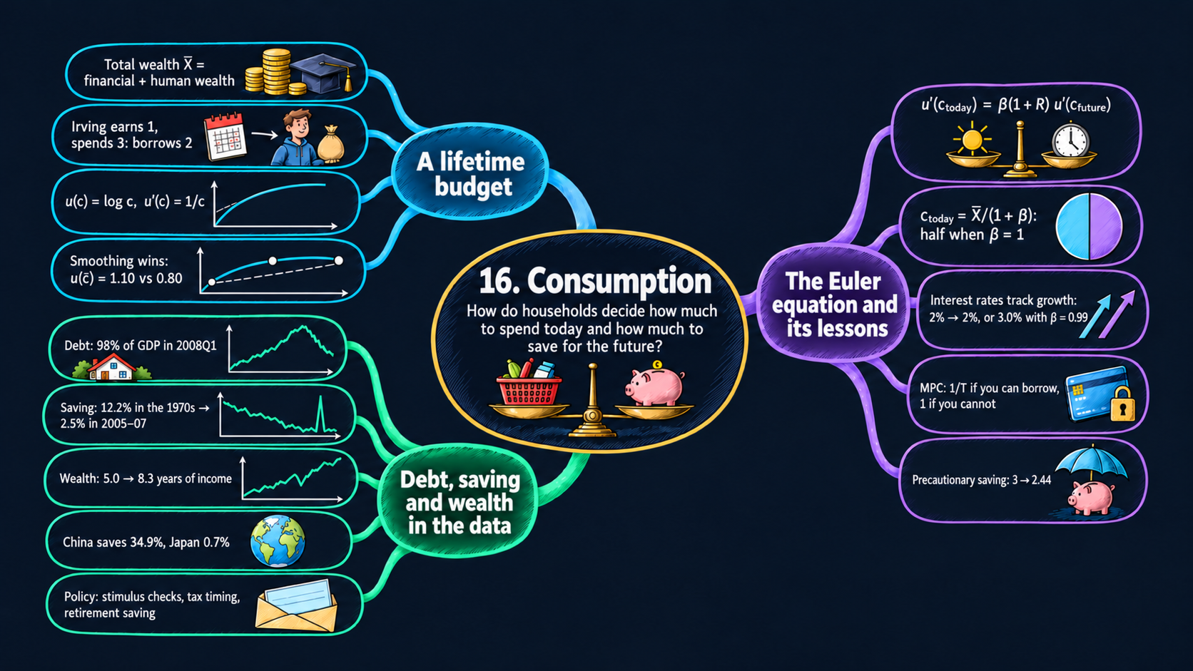
Consumption is more than two-thirds of GDP. Earlier chapters treated it simply, as a fixed share of income. This chapter asks how a household chooses to spend over its lifetime. By the end of it you will be able to:
- derive the intertemporal budget constraint from the budgets of the two periods, and split total wealth into financial wealth and human wealth;
- explain diminishing marginal utility, and why it makes people want to smooth consumption;
- derive the Euler equation in two ways, with a small-move argument and with calculus, and solve the two-period neoclassical consumption model with log utility for any degree of patience \(\beta\);
- compute the real interest rate that a given growth rate of consumption requires, and explain why interest rates and growth rates are numbers of similar size;
- read the comparative statics of consumption: the marginal propensities to consume, the wealth effect of the interest rate, and the income and substitution effects;
- extend the model to many periods and read it as the permanent-income and life-cycle hypotheses;
- compute the marginal propensity to consume with and without borrowing constraints, see why Ricardian equivalence can fail, and explain the random walk of consumption and precautionary saving;
- read data on household debt, the personal saving rate and household wealth, for the U.S. and dozens of other countries;
- in Python: write functions with text options, find a maximum on a grid with
np.argmax, turn monthly data into quarterly data withresample, join two tables withmerge, and fit a line through a scatter.
Model overview
Meet a young islander of Islandia. He is still a student and earns little today, but once he starts working he expects to earn five times as much. Should he live on his small income now, or borrow against his richer future? Earlier chapters made consumption a fixed share of income; this chapter turns it into a choice, and we follow this islander through every step. The figures and the code of this notebook call him Irving, after the economist Irving Fisher, who first studied this choice.
NoteThe big idea
The question. How does a household split its spending between today and the future, and why does it not simply spend what it earns each period?
The answer in one sentence. Because each extra unit of consumption is worth less than the one before, a household spreads its total wealth over its lifetime, and the Euler equation sets how steeply its consumption rises or falls.
What goes in and what comes out. We choose financial wealth, labor income in each period, the real interest rate and patience. The model gives back consumption in each period, saving or borrowing today, and the marginal propensity to consume out of extra income or a tax cut.
Road map.
- The two-period consumption model: the assumptions, solving the model step by step (lifetime budget, Euler equation, consumption plan, interest rate), and what the model predicts.
- Permanent income and the life cycle: the same logic over many periods, and saving for retirement.
- Taxes, borrowing constraints and uncertainty: Ricardian equivalence, the islander who cannot borrow, the random walk and precautionary saving.
- Model in code: the key results as Python functions, checked with numbers. The figures below reuse them.
Notation. As in the textbook, a bar marks total wealth \(\bar{X}\), a number the islander takes as given and cannot change; the other givens (\(f_{\text{today}}\), the incomes, \(R\) and \(\beta\)) carry no bar, and the model determines consumption.
| Symbol | Meaning | Type |
|---|---|---|
| \(c_{\text{today}}, c_{\text{future}}\) | consumption today and in the future | endogenous |
| \(f_{\text{future}}\) | financial wealth carried into the future (a debt if negative) | endogenous |
| \(U\) | lifetime utility | endogenous |
| \(g_c\) | growth rate of consumption, \((c_{\text{future}} - c_{\text{today}})/c_{\text{today}}\) | endogenous |
| \(f_{\text{today}}\) | financial wealth at the start: a bank balance, stocks, bonds | parameter |
| \(y_{\text{today}}, y_{\text{future}}\) | labor income today and in the future | parameters |
| \(R\) | the real interest rate | parameter |
| \(\beta\) | patience: the weight on future utility | parameter |
| \(\bar{X}\) | total wealth: financial wealth plus human wealth | parameter |
| \(T, W\) | periods of life and periods of work (second block) | parameters |
| \(\tau_{\text{today}}, \tau_{\text{future}}\) | taxes (third block) | parameters |
| \(u(c)\), \(u'(c)\) | flow utility, and marginal utility (a prime marks it) | notation |
| \(E[\cdot]\) | the average over the possible outcomes | notation |
The worked numbers use the baseline islander of every figure in this notebook: \(f_{\text{today}}=0\), \(y_{\text{today}}=1\), \(y_{\text{future}}=5\), \(\beta=1\), and \(R=0\) or \(R=0.05\). Think of one unit as 10,000 dollars.
The two-period consumption model
Assumptions
The islander’s life is cut into two periods. Six rules describe his choice.
1. Two periods. There is today, and there is the future. The future is his last period, so nothing should be left over at its end.
2. A budget in each period. Today he holds financial wealth \(f_{\text{today}}\) and earns labor income \(y_{\text{today}}\). Whatever he does not spend is added to his wealth, which becomes \(f_{\text{future}}\):
\[c_{\text{today}} + \underbrace{(f_{\text{future}} - f_{\text{today}})}_{\text{saving today}} = y_{\text{today}}.\]
In the future he earns \(y_{\text{future}}\), gets his savings back with interest, and spends it all:
\[c_{\text{future}} = y_{\text{future}} + (1+R)\,f_{\text{future}}.\]
Each budget reads “spending plus saving equals income” for its own period. Saving may be negative. Then \(f_{\text{future}} < 0\): the islander borrows today and repays \((1+R)\) times the loan in the future.
3. Free borrowing and lending. He can save or borrow any amount at one and the same real interest rate \(R\). The third block removes this rule.
4. Flow utility with diminishing marginal utility. Consuming \(c\) in a period yields \(u(c)\) units of utility. More consumption always helps, \(u'(c) > 0\), yet each extra unit helps less than the previous one: the marginal utility \(u'(c)\) falls as \(c\) grows. Our main case is log utility,
\[u(c) = \log c \qquad\text{with}\qquad u'(c) = \frac{1}{c},\]
where \(u'(c)\) is the derivative of the log (Appendix C.7). Our second case is the square root, \(u(c) = c^{1/2}\). By the power rule its marginal utility is \(u'(c) = \tfrac{1}{2}c^{-1/2} = 1/(2\sqrt{c})\). Fig. 1 plots both.
5. Lifetime utility. The islander sums the utility of both periods, and weighs the future by \(\beta\):
\[U = u(c_{\text{today}}) + \beta\,u(c_{\text{future}}). \tag{1}\]
The weight \(\beta\) is his patience. With \(\beta = 1\), a unit of utility counts the same today and later. With \(\beta < 1\), for example \(0.9\), he prefers to get it sooner.
6. Optimization. He picks \(c_{\text{today}}\) and \(c_{\text{future}}\) to make \(U\) as large as he can, subject to paying for the plan.
| Building block | Equation | Taken as given by the islander |
|---|---|---|
| budget today | \(c_{\text{today}} + (f_{\text{future}} - f_{\text{today}}) = y_{\text{today}}\) | \(f_{\text{today}}\), \(y_{\text{today}}\) |
| budget in the future | \(c_{\text{future}} = y_{\text{future}} + (1+R)f_{\text{future}}\) | \(y_{\text{future}}\), \(R\) |
| flow utility | \(u(c)\), with \(u'(c)\) falling in \(c\) | the shape of \(u\) |
| lifetime utility | \(U = u(c_{\text{today}}) + \beta u(c_{\text{future}})\) | \(\beta\) |
| behavior | choose \(c_{\text{today}}\), \(c_{\text{future}}\) to maximize \(U\) |
Extra consumption brings less and less utility, so the islander gains from spreading his spending evenly over his life.
NoteCheck your understanding
1. With log utility and \(\beta = 1\), the islander consumes 3 today and 3 in the future. What is his lifetime utility \(U\)?
Answer
By equation (1), \(U = \log 3 + 1 \times \log 3 = 2\log 3 \approx 2.197\).
2. With log utility, compare the marginal utility of the islander’s first unit of income today with that of his future income of 5. What does the comparison suggest he should do?
Answer
Rule 4 gives \(u'(1) = 1\) and \(u'(5) = 1/5 = 0.2\). A unit spent when he is poor (today) is worth five times a unit spent when he is rich (the future). So moving some spending from the future to today, by borrowing, raises his lifetime utility.
Solving the model
Step 1: one budget for a whole lifetime. The link between the two budgets is \(f_{\text{future}}\), the wealth carried from today into the future. Solve the future budget for it, by subtracting \(y_{\text{future}}\) and dividing by \(1+R\):
\[f_{\text{future}} = \frac{c_{\text{future}} - y_{\text{future}}}{1+R}.\]
Substitute it into today’s budget:
\[c_{\text{today}} + \frac{c_{\text{future}} - y_{\text{future}}}{1+R} - f_{\text{today}} = y_{\text{today}}.\]
Split the fraction into \(c_{\text{future}}/(1+R) - y_{\text{future}}/(1+R)\), and move \(f_{\text{today}}\) and the income terms to the right:
\[c_{\text{today}}+\frac{c_{\text{future}}}{1+R} \;=\; \underbrace{f_{\text{today}}}_{\text{financial wealth}}+\underbrace{y_{\text{today}}+\frac{y_{\text{future}}}{1+R}}_{\text{human wealth}}.\]
Dividing a future amount by \(1+R\) gives its present value (Appendix C.12). One dollar saved today becomes \(1+R\) dollars later, so \(1+R\) future dollars are worth one dollar now. Both sides are therefore present values.
ImportantKey result: the intertemporal budget constraint
\[c_{\text{today}}+\frac{c_{\text{future}}}{1+R} \;=\; f_{\text{today}}+y_{\text{today}}+\frac{y_{\text{future}}}{1+R} \;\equiv\; \bar{X} \tag{2}\]
The present value of lifetime spending (left) equals total wealth \(\bar{X}\) (right): financial wealth plus human wealth, the present value of labor income.
Islandia in numbers. For the baseline islander, \(\bar{X} = 0 + 1 + 5 = 6\) when \(R = 0\), and \(\bar{X} = 1 + 5/1.05 = 5.762\) when \(R = 0.05\).
TipIn words
Equation (2) does not ask the islander to pay for each period out of that period’s income. It asks only that the whole lifetime plan be paid for. So the student may spend more than he earns today, as long as his later wages can repay the loan with interest.
Read equation (2) as a straight line, with \(c_{\text{today}}\) on the horizontal axis: \(c_{\text{future}} = (1+R)(\bar{X} - c_{\text{today}})\). Its slope is \(-(1+R)\). Each unit eaten today costs \(1+R\) units later, so \(1+R\) is the price of consumption today, measured in future consumption.
Step 2: the condition for the best plan. We find it twice: with a thought experiment, then with calculus.
A small move. Take any affordable plan, and let the islander spend one unit less today and save it. Today he loses \(u'(c_{\text{today}})\) units of utility. The saved unit grows into \(1+R\) units in the future, each worth \(\beta\,u'(c_{\text{future}})\) in today’s utility. If the gain beats the loss, saving more raises \(U\). If the loss is larger, the reverse move (borrow one more unit and spend it today) raises \(U\). No move helps only when gain and loss are equal:
\[u'(c_{\text{today}}) = \beta(1+R)\,u'(c_{\text{future}}).\]
With calculus (Appendix C.8). The budget line lets us replace \(c_{\text{future}}\) by \((1+R)(\bar{X} - c_{\text{today}})\). Then lifetime utility depends on a single choice:
\[U(c_{\text{today}}) = u(c_{\text{today}}) + \beta\,u\big((1+R)(\bar{X}-c_{\text{today}})\big).\]
At the best \(c_{\text{today}}\), the derivative of \(U\) is zero. By the chain rule, the second term’s derivative is \(\beta\,u'(c_{\text{future}})\) times the derivative of the inside, which is \(-(1+R)\):
\[\frac{dU}{dc_{\text{today}}} = u'(c_{\text{today}}) - \beta(1+R)\,u'(c_{\text{future}}) = 0.\]
Both routes give the same condition. Because \(u'\) falls as consumption rises, the derivative is positive for a small \(c_{\text{today}}\) and negative for a large one, so its zero is a maximum.
ImportantKey result: the Euler equation
\[u'(c_{\text{today}}) = \beta(1+R)\,u'(c_{\text{future}}) \tag{3}\]
The value of spending one more unit today (left) equals the value of saving it for the future (right).
TipIn words
At the best plan, the islander does not care whether he spends or saves his last unit. Since marginal utility falls with consumption, the Euler equation also fixes the shape of the plan. When \(\beta(1+R) = 1\), it requires \(u'(c_{\text{today}}) = u'(c_{\text{future}})\), which means equal consumption in both periods.
Step 3: the Euler equation with log utility. Insert \(u'(c) = 1/c\) into equation (3):
\[\frac{1}{c_{\text{today}}} = \beta(1+R)\,\frac{1}{c_{\text{future}}}.\]
Multiply both sides by \(c_{\text{future}}\):
\[\frac{c_{\text{future}}}{c_{\text{today}}} = \beta(1+R). \tag{4}\]
The left side equals \(1 + g_c\), one plus the growth rate of consumption. Take logs of both sides (Appendix C.4): \(\log(1+g_c) = \log\beta + \log(1+R)\). For small \(x\), \(\log(1+x) \approx x\) (Appendix C.6), so
\[g_c \approx R + \log\beta.\]
Consumption grows faster when saving pays more (a higher \(R\)) and when the islander values the future more (a higher \(\beta\); with impatience, \(\log\beta < 0\) and growth is lower). Equation (4) sets the slope of the consumption path, not its level, and income is absent from it.
Step 4: solving for consumption. Equations (4) and (2) are two equations in the two unknowns. From (4), \(c_{\text{future}} = \beta(1+R)\,c_{\text{today}}\). Substitute this into (2); the factor \(1+R\) cancels:
\[c_{\text{today}} + \frac{\beta(1+R)\,c_{\text{today}}}{1+R} = c_{\text{today}} + \beta\,c_{\text{today}} = (1+\beta)\,c_{\text{today}} = \bar{X}.\]
Divide by \(1+\beta\), and go back to equation (4) for the future. The textbook case \(\beta = 1\) then has \(1+\beta = 2\).
ImportantKey result: the consumption plan with log utility
\[c_{\text{today}} = \frac{1}{1+\beta}\,\bar{X}, \qquad c_{\text{future}} = \frac{\beta(1+R)}{1+\beta}\,\bar{X} \tag{5}\]
\[c_{\text{today}} = \tfrac{1}{2}\,\bar{X}, \qquad c_{\text{future}} = \tfrac{1}{2}\,(1+R)\,\bar{X} \quad\text{when } \beta = 1 \tag{6}\]
Islandia in numbers. With \(R = 0\): \(c_{\text{today}} = c_{\text{future}} = 6/2 = 3\). The islander earns 1 but spends 3, so he borrows 2 and repays it out of his later 5. With \(R = 0.05\): \(c_{\text{today}} = 5.762/2 = 2.881\) and \(c_{\text{future}} = 1.05 \times 2.881 = 3.025\). He borrows \(1.881\), repays \(1.05 \times 1.881 = 1.975\), and has \(5 - 1.975 = 3.025\) left to spend.
TipIn words
With log utility, the islander spends a fixed share \(1/(1+\beta)\) of his total wealth today, whatever the interest rate and whenever his income arrives. A patient islander spends half; an impatient one spends more than half. What he does not spend today, he spends in the future, together with the interest it earned.
Step 5: the interest rate that matches a growth rate. The islander takes \(R\) as given and chooses how fast his consumption grows. For a whole economy the logic runs the other way. Growth models, such as the Solow–Romer model of Chapter 6, decide how fast output and consumption per person grow. The Euler equation then gives the real interest rate at which islanders are happy to consume along that path. Write \(1 + g_c\) for the left side of equation (4), divide by \(\beta\) and subtract 1:
\[1+R = \frac{1+g_c}{\beta}.\]
ImportantKey result: the interest rate that growth requires
\[R = \frac{1+g_c}{\beta} - 1 \tag{7}\]
Islandia in numbers. Let one period be a year, and let consumption grow by 2 percent a year, \(g_c = 0.02\). With \(\beta = 1\), \(R = 1.02 - 1 = 0.02\): the interest rate equals the growth rate, 2 percent. With \(\beta = 0.99\), \(R = 1.02/0.99 - 1 = 0.0303\), about 3.0 percent. The log approximation agrees: \(R \approx g_c - \log\beta = 0.02 + 0.01005\).
TipIn words
An impatient islander accepts a rising consumption path only if saving pays a premium of about \(-\log\beta\) a year. With \(\beta\) close to 1 the premium is small. That is why real interest rates and growth rates tend to be of the same size, a few percent a year. Faster growth raises the required interest rate about one for one.
Step 6: what a higher interest rate does. With log utility, \(R\) is absent from \(c_{\text{today}} = \bar{X}/(1+\beta)\). It acts only through total wealth: a higher \(R\) lowers the present value of future income, \(y_{\text{future}}/(1+R)\), and so lowers \(\bar{X}\) and \(c_{\text{today}}\). This is the wealth effect of the interest rate.
Beneath it, two forces push in opposite directions:
- The substitution effect. A higher \(R\) makes consumption today more expensive (its price is \(1+R\)), so the islander moves spending toward the future.
- The income effect. A saver earns more on his savings and can afford more in both periods, today included.
With log utility the two cancel exactly. To see it, take an islander whose wealth is all financial, \(y_{\text{today}} = y_{\text{future}} = 0\). Then \(\bar{X} = f_{\text{today}}\) does not depend on \(R\), and neither does \(c_{\text{today}} = f_{\text{today}}/(1+\beta)\).
With square-root utility they do not cancel. Insert \(u'(c) = 1/(2\sqrt{c})\) into equation (3); the factors \(1/2\) drop out:
\[\frac{1}{\sqrt{c_{\text{today}}}} = \beta(1+R)\frac{1}{\sqrt{c_{\text{future}}}} \quad\Longrightarrow\quad \sqrt{\frac{c_{\text{future}}}{c_{\text{today}}}} = \beta(1+R) \quad\Longrightarrow\quad \frac{c_{\text{future}}}{c_{\text{today}}} = \beta^2(1+R)^2.\]
Substitute \(c_{\text{future}} = \beta^2(1+R)^2 c_{\text{today}}\) into equation (2). One factor \(1+R\) cancels, and \(c_{\text{today}}\,[1 + \beta^2(1+R)] = \bar{X}\), so
\[c_{\text{today}} = \frac{\bar{X}}{1+\beta^2(1+R)}.\]
Now \(R\) also sits in the denominator: even with \(\bar{X}\) fixed, a higher \(R\) lowers \(c_{\text{today}}\), so the substitution effect wins. In general, the sign of the effect of \(R\) on consumption today depends on the shape of \(u\). For the baseline islander with \(R = 0.05\), square-root utility gives \(c_{\text{today}} = 5.762/2.05 = 2.811\), a bit below the 2.881 of log utility.
The islander spends a fixed share of his total wealth today; patience and the interest rate set how his consumption grows.
NoteCheck your understanding
1. The baseline islander faces \(R = 0.05\) but is less patient, \(\beta = 0.9\). How much does he consume today and in the future?
Answer
Total wealth is still \(\bar{X} = 5.762\). Equation (5) gives \(c_{\text{today}} = 5.762/1.9 \approx 3.033\) and \(c_{\text{future}} = 0.9 \times 1.05 \times 3.033 \approx 2.866\). Since \(\beta(1+R) = 0.945 < 1\), his consumption falls over time (equation 4).
2. His income is 1 today and 5 later, yet with \(R = 0\) and \(\beta = 1\) he consumes the same amount in both periods. Why does the timing of his income not matter?
Answer
Income enters only through total wealth \(\bar{X}\) in equation (2). The Euler equation (4) then sets \(c_{\text{future}}/c_{\text{today}} = \beta(1+R) = 1\), so consumption is flat. Borrowing and lending fill the gap between the income path and the consumption path.
What the model predicts
Comparative statics. Equation (5) tells us how each parameter moves consumption. Income and wealth enter \(\bar{X}\) linearly, so their effects are constants: the marginal propensities to consume (MPC), the rise in \(c_{\text{today}}\) per extra unit of resources. For \(R\) and \(\beta\), take logs of equation (5): \(\log c_{\text{today}} = \log\bar{X} - \log(1+\beta)\) and \(\log c_{\text{future}} = \log\beta + \log(1+R) + \log\bar{X} - \log(1+\beta)\). Let \(\sigma \equiv [y_{\text{future}}/(1+R)]/\bar{X}\) be the share of total wealth that comes from future income. A 1 percent rise in \(1+R\) cuts \(y_{\text{future}}/(1+R)\) by about 1 percent, and therefore cuts \(\bar{X}\) by about \(\sigma\) percent. A 1 percent rise in \(\beta\) raises \(1+\beta\) by \(\beta/(1+\beta)\) percent.
| Change | Effect on \(c_{\text{today}}\) | Effect on \(c_{\text{future}}\) | Baseline (\(\beta = 1\), \(R = 0.05\)) | The budget line |
|---|---|---|---|---|
| \(y_{\text{today}}\) or \(f_{\text{today}}\) up by 1 | \(+\dfrac{1}{1+\beta}\) | \(+\dfrac{\beta(1+R)}{1+\beta}\) | \(+0.5\) and \(+0.525\) | shifts out, same slope |
| \(y_{\text{future}}\) up by 1 | \(+\dfrac{1}{(1+\beta)(1+R)}\) | \(+\dfrac{\beta}{1+\beta}\) | \(+0.476\) and \(+0.5\) | shifts out, same slope |
| \(1+R\) up by 1% | \(-\sigma\) percent | \(+(1-\sigma)\) percent | \(-0.83\%\) and \(+0.17\%\) | pivots around the no-borrowing point |
| \(\beta\) up by 1% | \(-\dfrac{\beta}{1+\beta}\) percent | \(+\dfrac{1}{1+\beta}\) percent | \(-0.5\%\) and \(+0.5\%\) | does not move |
In the baseline, \(\sigma = 4.762/5.762 = 0.83\). The two elasticities for \(1+R\) differ by exactly 1, \((1-\sigma) - (-\sigma) = 1\), just as equation (4) demands: a 1 percent rise in \(1+R\) raises \(c_{\text{future}}/c_{\text{today}}\) by 1 percent. The “no-borrowing point” is the plan \(c_{\text{today}} = f_{\text{today}} + y_{\text{today}}\), \(c_{\text{future}} = y_{\text{future}}\), which is affordable at any interest rate.
The model’s main predictions.
- Consumption follows total wealth, not current income. Only \(\bar{X}\) matters, so a student with low income and bright prospects consumes far more than he earns.
- Windfalls are spread out. With \(\beta = 1\), one extra unit of income today raises consumption today by just one half; the other half is saved for later.
- Future income weighs a little less, because it is discounted by \(1+R\) before it enters total wealth.
- \(\beta(1+R)\) sets the growth of consumption (equation 4), whenever the income arrives.
- Interest rates and growth rates move together (equation 7): they are equal when \(\beta = 1\), and impatience adds a small premium.
- A higher interest rate lowers consumption today through the wealth effect when the islander has future labor income. Its full effect depends on the substitution and income effects, which cancel only with log utility.
Consumption tracks lifetime wealth, so a windfall today is shared between today and the future.
NoteCheck your understanding
1. With \(\beta = 1\) and \(R = 0.05\), the baseline islander receives a gift of 0.2 today. By how much do his consumption today and in the future rise?
Answer
The gift raises \(\bar{X}\) by 0.2. By equation (6), \(c_{\text{today}}\) rises by \(0.2/2 = 0.1\), and \(c_{\text{future}}\) by \(1.05 \times 0.1 = 0.105\). The MPC today is one half.
2. The interest rate rises. Why does the student’s consumption today fall, while that of an islander who lives on his bank balance alone does not change (log utility)?
Answer
By equation (5), \(c_{\text{today}}\) moves only with \(\bar{X}\). The student’s \(\bar{X}\) holds future wages, whose present value \(y_{\text{future}}/(1+R)\) falls: the wealth effect. The other islander’s \(\bar{X} = f_{\text{today}}\) does not depend on \(R\), and with log utility the substitution and income effects cancel.
Permanent income and the life cycle
Assumptions
Keep log utility and the Euler equation, but now the islander lives for \(T\) periods, \(t = 1, 2, \dots, T\), and earns \(y_1, y_2, \dots, y_T\). To keep the algebra simple, set \(R = 0\) and \(\beta = 1\). He still borrows and lends freely, and starts with financial wealth \(f_{\text{today}}\).
Solving the model
Step 1: a flat consumption path. The small-move argument of step 2 above works between any two neighboring periods. So equation (4) holds for every pair: \(c_{t+1}/c_t = \beta(1+R) = 1\), and consumption is the same number \(c\) in every period.
Step 2: the lifetime budget. With \(R = 0\) there is no discounting, and the budget of equation (2) is a plain sum. Lifetime spending, \(T \times c\), equals financial wealth plus all labor income, \(\bar{X} = f_{\text{today}} + y_1 + y_2 + \dots + y_T\). Divide by \(T\):
ImportantKey result: permanent income
\[c = \frac{\bar{X}}{T} = \frac{f_{\text{today}} + y_1 + y_2 + \dots + y_T}{T} \tag{8}\]
With \(T = 2\) this is equation (6) with \(R = 0\). An extra unit of income in a single period raises consumption by only \(1/T\); a raise of 1 in every period raises it by \(T/T = 1\).
TipIn words
In every period the islander spends the per-period average of his lifetime resources, his permanent income. A one-time windfall is spread over his whole life: with 40 periods left, he spends only \(1/40\) of it each period. A permanent raise, in contrast, is spent in full.
Step 3: saving for retirement. Let the islander work for the first \(W\) periods at income \(y\), then retire with no labor income for the last \(T - W\) periods. By equation (8), \(c = Wy/T\). While working he saves \(y - c = y(T-W)/T\) per period, so on the day he retires his wealth reaches \(W \times y(T-W)/T\). In retirement he lives on \(c\) out of that wealth until it hits zero in the last period. With \(T = 60\), \(W = 40\) and \(y = 1\): \(c = 40/60 = 0.667\), he saves \(0.333\) a year, and his wealth peaks at \(40 \times 0.333 = 13.3\), more than 13 years of income.
What the model predicts
- Permanent-income hypothesis (Friedman). Consumption depends on an average of lifetime resources, the present value of income, not on this period’s income. Temporary income changes move consumption little (MPC \(1/T\)); permanent ones move it a lot (MPC near 1).
- Expected changes do not move consumption when they arrive. A raise the islander saw coming is already in \(\bar{X}\), so his consumption does not jump on payday.
- Life-cycle hypothesis (Modigliani). Income has a hump over life while consumption is flat, so people save during their working years and draw down wealth in retirement. Wealth is hump-shaped as well, with its peak near retirement.
Islanders spend their permanent income: they save while working and live on their savings in retirement.
NoteCheck your understanding
1. An islander lives \(T = 60\) periods and works for \(W = 45\) of them at income 1, with \(R = 0\) and \(\beta = 1\). How much does he consume each period, how much does he save while working, and how high does his wealth climb?
Answer
By equation (8), \(c = 45/60 = 0.75\). He saves \(1 - 0.75 = 0.25\) in each working period, so his wealth peaks at \(45 \times 0.25 = 11.25\) on the day he retires: less than with 40 working periods, because his retirement is shorter.
2. The islander learns today that his wage will rise next year. When does his consumption go up: today, or when the raise is paid?
Answer
Today. The raise enters total wealth \(\bar{X}\) as soon as he knows about it, and equation (8) spreads it evenly over all periods. When the raise is finally paid, nothing new has happened, so his consumption does not jump.
Taxes, borrowing constraints and uncertainty
Assumptions
Return to two periods and log utility, and change one rule at a time.
1. Taxes. The Islandia Treasury collects taxes \(\tau_{\text{today}}\) and \(\tau_{\text{future}}\), so the incomes in the budgets are after-tax incomes, \(y_{\text{today}} - \tau_{\text{today}}\) and \(y_{\text{future}} - \tau_{\text{future}}\). The Treasury borrows and lends at the same rate \(R\) as the islander.
2. A borrowing constraint. The islander cannot borrow at all: \(f_{\text{future}} \ge 0\). Today’s budget gives \(f_{\text{future}} = f_{\text{today}} + y_{\text{today}} - c_{\text{today}}\), so the constraint reads \(c_{\text{today}} \le f_{\text{today}} + y_{\text{today}}\): he cannot spend more than he holds today. With no financial wealth, it is simply \(c_{\text{today}} \le y_{\text{today}}\).
3. Uncertainty. Future income is unknown today, and the islander maximizes expected lifetime utility.
Solving the model
Ricardian equivalence. With taxes, total wealth is
\[\bar{X} = f_{\text{today}} + (y_{\text{today}} - \tau_{\text{today}}) + \frac{y_{\text{future}} - \tau_{\text{future}}}{1+R}.\]
Suppose the Treasury cuts today’s tax by \(\Delta\) and borrows to fund the cut. It must repay \((1+R)\Delta\) in the future, so it raises the future tax by that amount. Total wealth changes by
\[\Delta\bar{X} = +\Delta - \frac{(1+R)\Delta}{1+R} = \Delta - \Delta = 0.\]
Since total wealth is unchanged, equation (5) says consumption is unchanged too. The islander saves the whole tax cut, and that saving, with its interest, pays exactly the higher future tax. This is Ricardian equivalence: for a given path of government spending, the timing of taxes does not matter.
The borrowing constraint. Whenever the plan of equation (5) is affordable today, it is still the best choice. When it is not, the islander gets as close to it as he can, by spending all he holds today:
ImportantKey result: consumption with a borrowing constraint
\[c_{\text{today}} = \min\left\{\frac{\bar{X}}{1+\beta},\; f_{\text{today}} + y_{\text{today}}\right\} \tag{9}\]
Islandia in numbers. The baseline islander with \(R = 0.05\) would like to spend 2.881 today but holds only 1. Constrained, he spends \(c_{\text{today}} = 1\), and \(c_{\text{future}} = y_{\text{future}} = 5\).
When does the constraint bind? Take \(\beta = 1\). The plan \(\bar{X}/2\) exceeds \(f_{\text{today}} + y_{\text{today}}\) exactly when
\[f_{\text{today}} + y_{\text{today}} + \frac{y_{\text{future}}}{1+R} > 2\,(f_{\text{today}} + y_{\text{today}}) \quad\Longleftrightarrow\quad \frac{y_{\text{future}}}{1+R} > f_{\text{today}} + y_{\text{today}}.\]
The constraint binds when the present value of future income exceeds what the islander holds today: he wants to borrow and cannot. The baseline islander is such a case, since \(5/1.05 = 4.76 > 1\).
TipIn words: when the constraint binds
A constrained islander already wishes he could spend more today. So he spends an extra unit of income today in full, an MPC of 1. Extra future income does nothing for him today. A tax cut today raises his consumption one for one, and Ricardian equivalence fails.
Uncertain income: the random walk. With risky future income the small-move argument still holds, but the gain from saving is now uncertain. So the expected marginal utility of the future is what must balance:
\[u'(c_{\text{today}}) = \beta(1+R)\,E\big[u'(c_{\text{future}})\big],\]
where \(E[\cdot]\) averages over the possible outcomes. If \(\beta(1+R) = 1\) and marginal utility is close to a straight line over the relevant range, the best forecast of next period’s consumption is this period’s: \(c_{\text{future}} = c_{\text{today}} + \text{surprise}\). All that the islander knows today is already in his consumption, so only news can move it. Robert Hall named this the random walk of consumption.
Uncertain income: precautionary saving. Marginal utility \(1/c\) is not a straight line: it is steeper at low consumption. So a spread of outcomes lifts the average of \(1/c_{\text{future}}\) above \(1/E[c_{\text{future}}]\). The bad outcome raises marginal utility by more than the good outcome lowers it. A larger right-hand side calls for a smaller \(c_{\text{today}}\), that is, more saving. A worked example with \(R = 0\), \(\beta = 1\) and the baseline incomes: let \(y_{\text{future}}\) be 3 or 7 with equal chances, instead of a sure 5. Then \(c_{\text{future}}\) is \(4 - c_{\text{today}}\) or \(8 - c_{\text{today}}\), and the expected Euler equation is
\[\frac{1}{c_{\text{today}}} = \frac{1}{2}\cdot\frac{1}{4 - c_{\text{today}}} + \frac{1}{2}\cdot\frac{1}{8 - c_{\text{today}}}.\]
Multiply both sides by \(c_{\text{today}}(4-c_{\text{today}})(8-c_{\text{today}})\) and collect terms (Appendix C.9): \(32 - 12c_{\text{today}} + c_{\text{today}}^2 = 6c_{\text{today}} - c_{\text{today}}^2\), or \(c_{\text{today}}^2 - 9c_{\text{today}} + 16 = 0\). The root below 4 is \(c_{\text{today}} = (9 - \sqrt{17})/2 = 2.44\). Risk cuts consumption today from 3 to 2.44, although future income is still 5 on average.
TipIn words: saving for a rainy day
A bad year hurts the islander more than a good year of the same size helps him, because marginal utility is steepest when consumption is low. So he insures himself by saving more today. The riskier his future wages, the more he puts aside.
What the model predicts
| The islander receives … | MPC today, can borrow (\(\beta = 1\)) | MPC today, borrowing-constrained |
|---|---|---|
| one more unit of income today | \(1/2\) | \(1\) |
| one more unit of income in the future | \(1/[2(1+R)]\) | \(0\) |
| a tax cut today, repaid by a tax rise later | \(0\) (Ricardian equivalence) | \(1\) |
- The timing of taxes does not matter for households that can borrow and that pay the later taxes themselves. It does matter when they are constrained, and when the later taxes fall on others, such as other income groups or future generations.
- Constrained households spend what they earn. Their consumption tracks current income, with an MPC of 1, far above the \(1/T\) of the permanent-income consumer. With both kinds of households, the economy’s average MPC lies in between.
- Consumption should be hard to predict. In the random walk view, expected income changes are already in today’s consumption, and only surprises move it.
- Risk makes people save, even on low incomes. Precautionary savers behave much like constrained households: their consumption also reacts strongly to current income.
Tax cuts, windfalls and risk matter most for islanders who cannot borrow: they spend what they get.
NoteCheck your understanding
1. With \(R = 0.05\), the Islandia Treasury cuts today’s tax by 0.1 and raises the future tax by 0.105. How does consumption today change for the baseline islander if he can borrow, and if he cannot?
Answer
If he can borrow, nothing changes: \(\Delta\bar{X} = 0.1 - 0.105/1.05 = 0\), so by equation (5) he still consumes 2.881 and saves the cut (Ricardian equivalence). If he cannot borrow, equation (9) binds, so he spends everything he holds: \(c_{\text{today}}\) rises from 1 to 1.1, an MPC of 1.
2. Future income is now 4 or 6 with equal chances, with \(R = 0\), \(\beta = 1\) and the baseline incomes. How much does the islander consume today? Compare with the sure case and with a spread of 3 or 7.
Answer
Now \(c_{\text{future}}\) is \(5 - c_{\text{today}}\) or \(7 - c_{\text{today}}\). The expected Euler equation, \(1/c_{\text{today}} = \tfrac{1}{2}/(5 - c_{\text{today}}) + \tfrac{1}{2}/(7 - c_{\text{today}})\), simplifies to \(2c_{\text{today}}^2 - 18c_{\text{today}} + 35 = 0\), whose root below 5 is \(c_{\text{today}} = (9 - \sqrt{11})/2 \approx 2.84\). That is below the 3 of the sure case but above the 2.44 of the wider spread: less risk, less precautionary saving.
NoteRecap
- Diminishing marginal utility makes an even consumption path better than an uneven one, so the islander wants to smooth (Fig. 1, Fig. 2).
- One lifetime budget: spending in present value equals total wealth \(\bar{X}\), financial plus human wealth (equation 2).
- The Euler equation \(u'(c_{\text{today}}) = \beta(1+R)\,u'(c_{\text{future}})\) sets the growth of consumption; with log utility, \(c_{\text{today}} = \bar{X}/(1+\beta)\) (Fig. 2).
- Interest rates and growth rates are linked by \(R = (1+g_c)/\beta - 1\), which is why both are a few percent a year.
- Permanent income and the life cycle: consumption follows lifetime resources, so households save while working and run down wealth in retirement (Fig. 5).
- Borrowing constraints and risk raise the MPC to 1 and break Ricardian equivalence; precautionary saving shows up in the data on saving and debt (Fig. 4, Fig. 3).
Model in code
Now we turn the Key results into Python. The section has three parts: the setup (folded, because it is the same in every chapter), the model as functions, and numerical checks of the Key results. Run its cells once, in order. Every later section of the notebook reuses them.
Setup
Run the setup cells once, before anything else. They load the Python libraries, give every chart the same look, store the address of the chapter’s data and define a helper that only the book website needs. You can use the notebook without reading them; open the box if you are curious.
NoteShow the setup code
The first cell loads the libraries and sets the look of the charts. Its comments explain each step.
The website cannot run Python, so each interactive figure also gets a version with a precomputed slider. The next helper builds those versions. Run it and move on.
# @title Helper for the website versions (run this cell; you do not need to read it)
def slider_figure(make_figure, name, values, start, label=None):
    """Join precomputed versions of a figure with one slider (the website cannot run Python).

    Arguments
        make_figure : the function that draws the figure, e.g. flow_utility
        name        : the argument the slider moves, e.g. "c"
        values      : the values of that argument to precompute
        start       : the value shown first
        label       : the slider's label (the argument name if None)
    Returns
        one Plotly figure with all versions and a slider that shows one at a time
    """
    # Step 1: draw the figure once for every value
    figures = [make_figure(**{name: v}) for v in values]
    first = values.index(start)
    # Step 2: copy every curve into one figure; only the start value's are visible
    fig = go.Figure(layout=figures[first].layout)
    owner = []                                  # which figure each trace comes from
    for i, f in enumerate(figures):
        for trace in f.data:
            trace.visible = (i == first)
            fig.add_trace(trace)
            owner.append(i)
    # Step 3: one slider step per value: its curves, title, labels and shapes
    steps = []
    for i, f in enumerate(figures):
        layout = {"title": f.layout.title.to_plotly_json(),
                  "annotations": [a.to_plotly_json() for a in f.layout.annotations],
                  "shapes": [s.to_plotly_json() for s in f.layout.shapes]}
        visible = [o == i for o in owner]
        steps.append(dict(method="update", label=str(values[i]), args=[{"visible": visible}, layout]))
    fig.update_layout(sliders=[dict(active=first, steps=steps, pad=dict(t=60),
                                    currentvalue=dict(prefix=(label or name) + " = "))])
    return fig
The model as functions
The model rests on lifetime utility, equation (1), and on what the islander can afford, equation (2). We write each piece as a Python function: a named recipe that takes inputs and gives back a result. The first three functions describe preferences: flow utility, marginal utility and lifetime utility.
# `def` creates a function. Its inputs are the arguments in parentheses.
# `form="log"` gives `form` a default value, used whenever we do not pass one.
# The text in triple quotes describes the function.
def utility(c, form="log"):
    """Flow utility u(c), the curve of Fig. 1.

    Log or square-root utility:  u(c) = log c,  or  u(c) = sqrt(c)

    Arguments
        c    : consumption (one number or a whole array of numbers)
        form : "log" (the default) or "square root"
    Returns
        flow utility u(c)
    """
    # `if ... :` runs the indented line only when the condition is true.
    # `return` gives back the result; np.log and np.sqrt work on a single
    # number and on a whole array alike.
    if form == "log":
        return np.log(c)
    return np.sqrt(c)


def marginal_utility(c, form="log"):
    """Marginal utility u'(c), the slope of the utility curve.

    Equation (3) uses it:  u'(c) = 1/c (log),  or  u'(c) = 1/(2 sqrt(c)) (square root)

    Arguments
        c    : consumption (one number or an array)
        form : "log" (the default) or "square root"
    Returns
        marginal utility u'(c)
    """
    # the slope falls as c rises: diminishing marginal utility
    if form == "log":
        return 1 / c
    return 1 / (2 * np.sqrt(c))


def lifetime_utility(c_today, c_future, beta=1.0, form="log"):
    """Lifetime utility of a consumption plan.

    Equation (1):  U = u(c_today) + beta u(c_future)

    Arguments
        c_today, c_future : consumption today and in the future
        beta              : patience, the weight on future utility (1 unless we pass another)
        form              : "log" (the default) or "square root"
    Returns
        lifetime utility, U
    """
    # future utility counts with the weight beta
    return utility(c_today, form) + beta * utility(c_future, form)
The next three functions hold the solution with log utility: total wealth, the consumption plan and the interest rate that goes with a growth rate of consumption.
def total_wealth(f_today, y_today, y_future, R):
    """Total wealth, financial plus human wealth.

    Equation (2):  X-bar = f_today + y_today + y_future / (1 + R)

    Arguments
        f_today            : financial wealth today
        y_today, y_future  : labor income today and in the future
        R                  : the real interest rate
    Returns
        total wealth, X-bar
    """
    # future income counts at its present value, divided by 1 + R
    return f_today + y_today + y_future / (1 + R)


def consumption_plan(f_today, y_today, y_future, R, beta=1.0):
    """Irving's best consumption plan with log utility.

    Equations (5) and (6):  c_today = X-bar / (1 + beta),  c_future = beta (1 + R) c_today

    Arguments
        f_today            : financial wealth today
        y_today, y_future  : labor income today and in the future
        R                  : the real interest rate
        beta               : patience (1 unless we pass another value)
    Returns
        c_today, c_future : consumption today and in the future
    """
    # Step 1: total wealth, equation (2)
    X = total_wealth(f_today, y_today, y_future, R)
    # Step 2: consume the share 1/(1 + beta) of it today, equation (5)
    c_today = X / (1 + beta)
    # Step 3: the Euler equation (4) gives the future; a function can `return`
    # two results at once, separated by a comma
    return c_today, beta * (1 + R) * c_today


def euler_interest_rate(g, beta=1.0):
    """The real interest rate that makes consumption grow at rate g.

    Equation (7):  R = (1 + g) / beta - 1

    Arguments
        g    : the growth rate of consumption, g_c
        beta : patience (1 unless we pass another value)
    Returns
        the real interest rate, R
    """
    # equation (4) solved for R, with c_future / c_today = 1 + g
    return (1 + g) / beta - 1
Checking the key results
The shared baseline. The textbook gives no numbers for its diagrams, so every figure of this notebook starts from the illustrative Irving of the notation paragraph: \(f_{\text{today}}=0\), \(y_{\text{today}}=1\), \(y_{\text{future}}=5\), and \(\beta=1\), \(R=0\), as in the caption of the textbook’s Fig. 16.2. We compute his total wealth, his plan and his lifetime utility.
# Step 1: the shared baseline; one line can give values to three names at once
f_today, y_today, y_future = 0.0, 1.0, 5.0      # the shared baseline
# Step 2: total wealth (2) and the plan (5) with R = 0. `c_today, c_future = ...`
# unpacks the two results of the function into two names.
X = total_wealth(f_today, y_today, y_future, R=0.0)
c_today, c_future = consumption_plan(f_today, y_today, y_future, R=0.0)
# Step 3: show the results. An f-string, f"... {X:.2f}", puts a value into the
# text; ":.2f" means "two decimals", and ":+.2f" also shows the sign.
print(f"Total wealth X = {X:.2f}  (financial {f_today:.2f} + human {X - f_today:.2f})")
print(f"Consumption today {c_today:.2f}, in the future {c_future:.2f}")
print(f"Saving today = y_today - c_today = {y_today - c_today:+.2f}  (negative: Irving borrows)")
print(f"Lifetime utility U = {lifetime_utility(c_today, c_future):.3f}")
Total wealth X = 6.00 (financial 0.00 + human 6.00)
Consumption today 3.00, in the future 3.00
Saving today = y_today - c_today = -2.00 (negative: Irving borrows)
Lifetime utility U = 2.197Irving earns 1 today but consumes 3: he borrows 2 against his future income and repays it from the 5 he earns later.
Check 1: the solution without calculus. The formula \(c_{\text{today}}=\bar{X}/(1+\beta)\) came from the Euler equation. We can also let the computer search for the best choice. Every \(c_{\text{today}}\) on a fine grid leaves \(c_{\text{future}}=(1+R)(\bar{X}-c_{\text{today}})\) for the future; we compute lifetime utility for each one and pick the largest. We use \(R=0.05\), so that the future is not a copy of today, and try a patient (\(\beta = 1\)) and a less patient (\(\beta = 0.9\)) Irving. For each, we also plug the plan into both sides of the Euler equation (3) and of the budget (2).
# Step 1: total wealth at R = 5%, and a grid of candidates for c_today.
# np.linspace(a, b, n) makes n evenly spaced numbers from a to b.
R = 0.05
X = total_wealth(f_today, y_today, y_future, R)
grid = np.linspace(0.01, X - 0.01, 100001)          # candidate values of c_today
# Step 2: a `for` loop runs its indented lines once for each element of the
# list, here once for each value of beta
for beta in [1.0, 0.9]:
    # arithmetic on an array works element by element, so U has one lifetime
    # utility per candidate; np.argmax gives the position of the largest one
    U = lifetime_utility(grid, (1 + R) * (X - grid), beta)
    best = np.argmax(U)
    c_today, c_future = consumption_plan(f_today, y_today, y_future, R, beta)
    # Step 3: compare; grid[best] is the candidate at that position
    print(f"beta = {beta}: grid search c_today = {grid[best]:.4f},  formula (5) X/(1 + beta) = {c_today:.4f}")
    # both sides of the Euler equation (3), (4), and of the budget (2)
    print(f"   Euler (3): u'(c_today) = {marginal_utility(c_today):.4f},  "
          f"beta (1 + R) u'(c_future) = {beta * (1 + R) * marginal_utility(c_future):.4f}")
    print(f"   Euler (4): c_future / c_today = {c_future / c_today:.4f},  beta (1 + R) = {beta * (1 + R):.4f}")
    print(f"   Budget (2): c_today + c_future/(1 + R) = {c_today + c_future / (1 + R):.4f},  X = {X:.4f}")
beta = 1.0: grid search c_today = 2.8810, formula (5) X/(1 + beta) = 2.8810
Euler (3): u'(c_today) = 0.3471, beta (1 + R) u'(c_future) = 0.3471
Euler (4): c_future / c_today = 1.0500, beta (1 + R) = 1.0500
Budget (2): c_today + c_future/(1 + R) = 5.7619, X = 5.7619
beta = 0.9: grid search c_today = 3.0326, formula (5) X/(1 + beta) = 3.0326
Euler (3): u'(c_today) = 0.3298, beta (1 + R) u'(c_future) = 0.3298
Euler (4): c_future / c_today = 0.9450, beta (1 + R) = 0.9450
Budget (2): c_today + c_future/(1 + R) = 5.7619, X = 5.7619The search and the formula agree, and both sides of the Euler equation and of the budget are equal. With \(\beta = 1\) and \(R=0.05\) consumption grows by 5 percent from today to the future, exactly \(\beta(1+R)=1.05\). The less patient Irving spends more today and lets consumption fall a little, since \(0.9 \times 1.05 = 0.945 < 1\).
Check 2: the interest rate for 2 percent growth. Equation (7) gives the real interest rate that makes consumption grow by 2 percent a year. We compute it for \(\beta = 1\) and \(\beta = 0.99\), compare it with the log approximation \(R \approx g_c - \log\beta\), and plug it back into the Euler equation (4).
# For a patient and a slightly less patient Irving: R from equation (7), its
# log approximation, and the growth of consumption that this R implies
g = 0.02                                             # growth of consumption per year
for beta in [1.0, 0.99]:
    R_needed = euler_interest_rate(g, beta)
    approx = g - np.log(beta)                        # the log approximation of step 3
    growth = beta * (1 + R_needed) - 1               # plug R back into equation (4)
    print(f"beta = {beta}: R = {100 * R_needed:.2f}%  (approximation {100 * approx:.2f}%),  "
          f"implied consumption growth = {100 * growth:.2f}%")
beta = 1.0: R = 2.00% (approximation 2.00%), implied consumption growth = 2.00%
beta = 0.99: R = 3.03% (approximation 3.01%), implied consumption growth = 2.00%Check 3: the elasticities. The table of comparative statics predicts that a 1 percent rise in \(1+R\) changes \(c_{\text{today}}\) by \(-\sigma\) percent and \(c_{\text{future}}\) by \(1-\sigma\) percent, and that a 1 percent rise in \(\beta\) lowers \(c_{\text{today}}\) by \(\beta/(1+\beta) = 0.5\) percent. We raise each by 1 percent and compare.
# Step 1: the plan at R = 5%, then with 1 + R and with beta 1 percent higher
R = 0.05
base_today, base_future = consumption_plan(f_today, y_today, y_future, R)
new_R = 1.01 * (1 + R) - 1                           # 1 + R is 1 percent higher
R_today, R_future = consumption_plan(f_today, y_today, y_future, new_R)
beta_today, beta_future = consumption_plan(f_today, y_today, y_future, R, beta=1.01)
# Step 2: sigma, the share of future income in total wealth
sigma = (y_future / (1 + R)) / total_wealth(f_today, y_today, y_future, R)
# Step 3: the changes in percent, next to the predictions
print(f"Share of future income in total wealth: sigma = {sigma:.3f}")
print(f"1% higher 1 + R: c_today {100 * (R_today / base_today - 1):+.3f}%  (predicted {-sigma:+.3f}%)")
print(f"                 c_future {100 * (R_future / base_future - 1):+.3f}%  (predicted {1 - sigma:+.3f}%)")
print(f"1% higher beta:  c_today {100 * (beta_today / base_today - 1):+.3f}%  (predicted -0.500%)")
Share of future income in total wealth: sigma = 0.826
1% higher 1 + R: c_today -0.818% (predicted -0.826%)
c_future +0.174% (predicted +0.174%)
1% higher beta: c_today -0.498% (predicted -0.500%)The numbers are close to the predictions but not identical for \(c_{\text{today}}\), because an elasticity describes very small changes and 1 percent is small but not zero. The effect on \(c_{\text{future}}\) is exact here, since \(c_{\text{future}}\) is a straight-line function of \(1+R\).
Check 4: income and substitution effects. First a grid search confirms the square-root formula \(c_{\text{today}} = \bar{X}/[1+\beta^2(1+R)]\). Then we take an Irving whose wealth is all financial, \(f_{\text{today}} = 6\) with no labor income, and raise the interest rate. With log utility the two effects cancel, so \(c_{\text{today}}\) should not move. With square-root utility the substitution effect wins, so it should fall.
# Step 1: grid search with square-root utility at R = 5%, against the formula
R = 0.05
X = total_wealth(f_today, y_today, y_future, R)
grid = np.linspace(0.01, X - 0.01, 100001)
U = lifetime_utility(grid, (1 + R) * (X - grid), 1.0, "square root")
print(f"Square root, baseline: grid search c_today = {grid[np.argmax(U)]:.4f},  "
      f"formula X/(1 + beta^2 (1 + R)) = {X / (1 + 1.0 ** 2 * (1 + R)):.4f}")
# Step 2: all wealth financial; raise R and watch c_today under both utilities.
# `[0]` keeps only the first of the two results, c_today.
print("All wealth financial (f_today = 6, no labor income), beta = 1:")
for rate in [0.0, 0.05, 0.10]:
    log_today = consumption_plan(6.0, 0.0, 0.0, rate)[0]
    root_today = 6.0 / (1 + (1 + rate))            # the square-root formula, beta = 1
    print(f"   R = {rate:.2f}: c_today = {log_today:.3f} with log utility,  {root_today:.3f} with square root")
Square root, baseline: grid search c_today = 2.8107, formula X/(1 + beta^2 (1 + R)) = 2.8107
All wealth financial (f_today = 6, no labor income), beta = 1:
R = 0.00: c_today = 3.000 with log utility, 3.000 with square root
R = 0.05: c_today = 3.000 with log utility, 2.927 with square root
R = 0.10: c_today = 3.000 with log utility, 2.857 with square rootCheck 5: permanent income and the life cycle. We follow the worker of the second block, 40 working periods and 20 in retirement, with \(R = 0\). Consumption comes from equation (8); wealth is updated period by period. It should peak at 13.3 on the day of retirement and end at exactly zero. Then we give him an extra 0.01 in a single year: consumption should rise by \(0.01/60\), an MPC of \(1/60\).
# Step 1: income over the life. np.zeros(T) makes an array of T zeros, and
# `income[:W] = 1.0` sets its first W elements to 1.
# 60 periods of life, of which the first 40 are working years
T, W = 60, 40
income = np.zeros(T)
# labor income 1 while working, 0 in retirement
income[:W] = 1.0
# Step 2: consumption from equation (8); `.sum()` adds up all elements
c = income.sum() / T                                 # equation (8) with f_today = 0
# Step 3: follow wealth period by period. `range(T)` counts 0, 1, ..., T - 1,
# `income[t]` is element number t, and `max(a, b)` is the larger of two numbers.
wealth, peak = 0.0, 0.0
for t in range(T):
    wealth = wealth + income[t] - c      # R = 0: saving adds to wealth one for one
    peak = max(peak, wealth)
print(f"Consumption every period c = {c:.3f},  saving while working = {1 - c:.3f}")
print(f"Peak wealth = {peak:.2f}  (formula W (T - W)/T = {W * (T - W) / T:.2f}),  wealth at the end = {wealth:.6f}")
# Step 4: a one-time extra 0.01 in period 10, and the MPC out of it
income[10] = income[10] + 0.01
print(f"MPC out of a one-time windfall = {(income.sum() / T - c) / 0.01:.4f}  (1/T = {1 / T:.4f})")
Consumption every period c = 0.667, saving while working = 0.333
Peak wealth = 13.33 (formula W (T - W)/T = 13.33), wealth at the end = 0.000000
MPC out of a one-time windfall = 0.0167 (1/T = 0.0167)Check 6: Ricardian equivalence and the borrowing constraint. A tax cut of 0.01 today, repaid with interest by a tax rise later, should leave total wealth unchanged. Then we apply equation (9) to two Irvings: the baseline one, whose discounted future income is larger than what he has today, and one with income 4 today and 2 in the future, who wants to save anyway.
# Step 1: Ricardian equivalence: total wealth before and after the tax cut
R, cut = 0.05, 0.01
X_before = total_wealth(f_today, y_today, y_future, R)
# after-tax incomes: 0.01 more today, 0.01 (1 + R) less in the future
X_after = total_wealth(f_today, y_today + cut, y_future - (1 + R) * cut, R)
print(f"Tax cut today, tax rise later: total wealth {X_before:.6f} before, {X_after:.6f} after")
# Step 2: the borrowing constraint, equation (9). The loop hands over one pair
# of incomes at a time and unpacks it into the two names y_now and y_later.
for y_now, y_later in [(1.0, 5.0), (4.0, 2.0)]:
    plan = consumption_plan(0.0, y_now, y_later, R)[0]
    cash = 0.0 + y_now                               # f_today + y_today
    # a comparison such as `>` gives True or False: does the constraint bind?
    binds = y_later / (1 + R) > cash
    # `min(a, b)` is the smaller of two numbers: c_today from equation (9)
    print(f"y_today = {y_now}, y_future = {y_later}: plan {plan:.3f}, cash today {cash:.3f}, "
          f"binds: {binds}, c_today = {min(plan, cash):.3f}")
Tax cut today, tax rise later: total wealth 5.761905 before, 5.761905 after
y_today = 1.0, y_future = 5.0: plan 2.881, cash today 1.000, binds: True, c_today = 1.000
y_today = 4.0, y_future = 2.0: plan 2.952, cash today 4.000, binds: False, c_today = 2.952Check 7: precautionary saving. Future income is 3 or 7 with equal chance, instead of a sure 5, with \(R = 0\) and \(\beta = 1\). A grid search over \(c_{\text{today}}\) maximizes expected lifetime utility. It should find \((9-\sqrt{17})/2 \approx 2.44\), below the 3 of the sure case, and the plan should satisfy the expected Euler equation.
# Step 1: candidates for c_today; below 4 keeps consumption positive in the bad case
grid = np.linspace(0.01, 3.99, 100001)
saving = y_today - grid                              # f_today = 0 and R = 0
# Step 2: lifetime utility with a sure income, and expected lifetime utility
# with income 3 or 7, each with probability 1/2
sure = np.log(grid) + np.log(5.0 + saving)
risky = np.log(grid) + 0.5 * np.log(3.0 + saving) + 0.5 * np.log(7.0 + saving)
# Step 3: the best candidate in each case, and the difference
c_sure, c_risky = grid[np.argmax(sure)], grid[np.argmax(risky)]
print(f"Sure future income 5:     c_today = {c_sure:.4f}")
print(f"Future income 3 or 7:     c_today = {c_risky:.4f}   (formula (9 - sqrt 17)/2 = {(9 - np.sqrt(17)) / 2:.4f})")
print(f"Precautionary saving = {c_sure - c_risky:.4f}")
# Step 4: the expected Euler equation, 1/c_today = average of 1/c_future
low, high = 3.0 + y_today - c_risky, 7.0 + y_today - c_risky
print(f"Expected Euler: 1/c_today = {1 / c_risky:.4f},  average of 1/c_future = {0.5 / low + 0.5 / high:.4f}")
Sure future income 5: c_today = 3.0000
Future income 3 or 7: c_today = 2.4384 (formula (9 - sqrt 17)/2 = 2.4384)
Precautionary saving = 0.5616
Expected Euler: 1/c_today = 0.4101, average of 1/c_future = 0.4101Utility and the desire to smooth consumption
Two diagrams explain why people spread their spending over time: the shape of the utility function, and what that shape implies when income is uneven.
Fig. 1: Flow utility
Goal. See diminishing marginal utility: each extra unit of consumption adds less utility than the one before.
The curve is the textbook’s \(u(c)=\log c\). Its slope at any point is the marginal utility \(u'(c)=1/c\). The figure marks one consumption level and draws the tangent line there, whose slope is \(u'(c)\). As \(c\) grows, the curve, and the tangent with it, becomes flatter and flatter.
First we compute the three numbers the figure reports. utility_at gives the utility \(u(c)\), the marginal utility \(u'(c)\), the slope of the tangent, and the utility that one more unit of consumption adds.
def utility_at(c, form="log"):
    """Utility, marginal utility and the gain from one more unit at c (Fig. 1).

    u(c), its slope u'(c) (1/c with log utility, as in equation 3), and u(c + 1) - u(c)

    Arguments
        c    : consumption, c
        form : "log" (the default) or "square root"
    Returns
        u    : flow utility, u(c)
        mu   : marginal utility, u'(c): the slope of the tangent at c
        gain : the utility added by one more unit, u(c + 1) - u(c)
    """
    # utility and its slope at c (functions of Model in code)
    u, mu = utility(c, form), marginal_utility(c, form)
    # utility added by one more unit: a little less than mu, since the curve flattens
    gain = utility(c + 1, form) - u
    return u, mu, gain
Show the drawing code
# @title Drawing code: Fig. 1, the names of the curve and of the slope
def label_utility(fig, form, mu):
    """The two labels of Fig. 1: the name of the curve and the slope of the tangent.

    Arguments
        fig  : the figure to write on
        form : "log" or "square root", the utility function
        mu   : marginal utility at the chosen c, u'(c)
    """
    # `add_annotation` writes a text label at a point: the curve's name at its
    # right end, as the textbook does
    name = {"log": "u(c) = log c", "square root": "u(c) = √c"}[form]
    fig.add_annotation(
        x=10,
        y=utility(10, form),
        text=name,
        showarrow=False,
        xanchor="right",
        yshift=16,
    )
    # the slope of the tangent, in a corner that stays empty for every c
    fig.add_annotation(
        x=10,
        y=-2,
        text=f"slope of the tangent: u′(c) = {mu:.2f}",
        showarrow=False,
        xanchor="right",
        font=dict(size=13, color=GREEN),
    )
Show the drawing code
# @title Drawing code: Fig. 1, flow utility and the tangent at c
def flow_utility(c=2.0, form="log"):
    """Flow utility u(c), with the tangent at c, whose slope is the marginal utility.

    Draws Fig. 1 (adapted from Fig. 16.1 in Jones).

    Arguments
        c    : consumption, c, where the tangent touches the curve
        form : "log" (the default) or "square root"
    Returns
        a Plotly figure
    """
    # Step 1: the numbers of the figure (utility_at)
    u, mu, gain = utility_at(c, form)
    # the curve from 0.01 to 10 (log c has no value at 0)
    grid = np.linspace(0.01, 10, 1000)
    # a short stretch around c for the tangent, inside the chart
    near = np.linspace(max(c - 2, 0.01), min(c + 2, 10.5), 50)

    # Step 2: `go.Figure()` starts an empty chart, and each `add_trace` adds one
    # curve or set of points. First the utility curve u(c)
    fig = go.Figure()
    fig.add_trace(
        go.Scatter(
            x=grid,
            y=utility(grid, form),
            name="u(c)",
            line=dict(color=BLUE, width=4),
        )
    )
    # the dashed tangent at c: u(c) + u'(c) (x - c), whose slope is u'(c)
    fig.add_trace(
        go.Scatter(
            x=near,
            y=u + mu * (near - c),
            name="tangent",
            mode="lines",
            line=dict(color=GREEN, width=2, dash="dash"),
        )
    )
    # the black dot at the chosen c
    fig.add_trace(
        go.Scatter(
            x=[c],
            y=[u],
            name="chosen c",
            mode="markers",
            marker=dict(color="black", size=11),
        )
    )
    label_utility(fig, form, mu)

    # Step 3: the title reports u(c), u'(c) and the gain from one more unit. Fixed
    # axis ranges, so that you can see what changes when you move a slider
    fig.update_layout(
        title=(
            f"c = {c:.1f}:  u(c) = {u:.2f},  marginal utility u′(c) = {mu:.2f},  "
            f"one more unit adds {gain:.2f}"
        ),
        showlegend=False,
        xaxis=dict(title="Consumption, c", range=[0, 10.5]),
        yaxis=dict(title="Utility", range=[-2.5, 3.5]),
    )
    return fig
Now the interactive version. Move the consumption slider and watch the tangent flatten.
# Fig. 1 with a slider and buttons. `interact` turns each argument of flow_utility
# into a widget and calls the function again every time you move one;
# `ToggleButtons` is a row of buttons for a choice between a few options. The `;`
# at the end only hides an extra line of text.
interact(
    flow_utility,
    c=FloatSlider(value=2.0, min=0.5, max=9.5, step=0.5,
                  description="consumption c", style=WIDE),
    form=ToggleButtons(options=["log", "square root"], value="log",
                       description="utility"),
);
Show the code of the website version
# @title Website version: Fig. 1 with a precomputed slider for consumption
# one picture of Fig. 1 per value of c; the slider shows one at a time
slider_figure(
    flow_utility,
    "c",
    [0.5, 1.0, 1.5, 2.0, 3.0, 4.0, 5.0, 6.0, 8.0, 9.5],     # the values of c
    start=2.0,
    label="consumption c",
)
Source. Adapted from Fig. 16.1 in Jones (2024), Macroeconomics, 6th ed.
What to notice.
- Utility always rises with consumption, but by less and less. At \(c=1\) the slope is \(1/1=1\); at \(c=2\) it is \(0.50\); at \(c=8\) it is only \(0.125\).
- The title compares the slope with the utility of one whole extra unit. Going from 2 to 3 adds \(\log 3-\log 2 = 0.41\), a little less than the slope at 2, because the curve keeps flattening along the way.
- The log curve has no floor: as \(c\) approaches zero, \(\log c\) falls without limit. Very low consumption is very painful, which is a strong reason to avoid it in any period.
- The square-root curve has the same basic shape, rising and flattening. Any such concave curve shows diminishing marginal utility.
Your turn. With log utility, find the consumption level at which marginal utility is exactly \(0.25\). Then check it in the empty cell with marginal_utility.
Hint
With log utility \(u'(c)=1/c\), so solve \(1/c = 0.25\). Then call marginal_utility(...) with your answer.
# Your turn: try it hereFig. 2: The desire to smooth consumption
Goal. See why diminishing marginal utility makes Irving prefer the same consumption in both periods to an uneven path with the same total.
Suppose Irving simply spent his income each period: \(c_1=y_{\text{today}}=1\) and \(c_2=y_{\text{future}}=5\). Or he could consume the average \(\bar{c}=(c_1+c_2)/2=3\) in both periods. With \(\beta=1\) and \(R=0\) both paths cost the same, and \(\bar{c}=3\) is exactly the solution \(\bar{X}/2\) of equation (6). Which path gives more utility?
- The uneven path gives the average utility \(\tfrac{1}{2}[u(c_1)+u(c_2)]\), the midpoint of the dashed line between the two points on the curve (the open circle).
- The smooth path gives \(u(\bar{c})\) in each period, the point on the curve above \(\bar{c}\) (the filled dot in the middle).
Because the curve bends, the point on the curve lies above the dashed line, so smoothing wins. Lifetime utility, twice these numbers, is higher with the smooth path.
The diagram draws dotted guides from each point down to the consumption axis. A small function adds one guide with its label, so that the figure function stays short.
Show the drawing code
# @title Drawing code: Fig. 2, a dotted guide down to the consumption axis
def add_guide(fig, x, top, label):
    """A dotted line from the consumption axis up to the point (x, top).

    Fig. 2 draws one under c1, c-bar and c2, with a label at the axis.

    Arguments
        fig   : the figure to draw on
        x     : the consumption level, on the horizontal axis
        top   : the height of the point: its utility
        label : the text at the axis ("" for none)
    Returns
        the same figure, with the guide added
    """
    # `add_shape` draws a line: from the bottom of the chart (-2.5) up to the point
    fig.add_shape(
        type="line",
        x0=x,
        x1=x,
        y0=-2.5,
        y1=top,
        line=dict(color=GRAY, width=1, dash="dot"),
    )
    # the label at the axis, unless it is empty
    if label:
        fig.add_annotation(
            x=x,
            y=-2.5,
            text=label,
            showarrow=False,
            yanchor="bottom",
            xshift=10,
            font=dict(size=15),
        )
    return fig
Then we compute the numbers the figure compares. smoothing_gain gives the smooth consumption \(\bar{c}\), the utility of each consumption level, and the average utility of the uneven path.
def smoothing_gain(c1, c2, form="log"):
    """The smooth path against the uneven one, in utility (Fig. 2).

    With beta = 1 and R = 0:  c-bar = (c1 + c2) / 2, and the average utility of the
    uneven path is [u(c1) + u(c2)] / 2. The gain from smoothing is u(c-bar) minus it.

    Arguments
        c1, c2 : consumption today and in the future on the uneven path
        form   : "log" (the default) or "square root"
    Returns
        c_bar          : the same consumption in both periods, c-bar
        u1, u2, u_bar  : the utility of c1, of c2 and of c-bar
        average        : the average utility of the uneven path
    """
    # the same consumption in both periods, with the same total
    c_bar = (c1 + c2) / 2
    # the utility of each consumption level
    u1, u2, u_bar = utility(c1, form), utility(c2, form), utility(c_bar, form)
    # the average utility of the uneven path
    average = (u1 + u2) / 2
    return c_bar, u1, u2, u_bar, average
Show the drawing code
# @title Drawing code: Fig. 2, the points, their labels and the guides
def smoothing_points(fig, c1, c2, c_bar, u1, u2, u_bar, average):
    """The points of Fig. 2: u(c1), u(c-bar), u(c2) and the average utility.

    Black dots on the curve, an open circle for the average utility of the uneven
    path, and dotted guides down to the consumption axis (add_guide).

    Arguments
        fig            : the figure to draw on
        c1, c2, c_bar  : consumption today, in the future, and smooth
        u1, u2, u_bar  : their utilities
        average        : the average utility of the uneven path
    """
    # Step 1: the three points on the curve; only u(c-bar) gets a label
    fig.add_trace(
        go.Scatter(
            x=[c1, c_bar, c2],
            y=[u1, u_bar, u2],
            mode="markers+text",
            text=["", "u(c̄)", ""],
            textposition="top left",
            marker=dict(color="black", size=11),
        )
    )
    # Step 2: the open circle: average utility, the midpoint of the dashed line
    side = "bottom right"
    if c_bar > 8.5:
        side = "bottom left"    # near the right edge: keep the label inside the chart
    fig.add_trace(
        go.Scatter(
            x=[c_bar],
            y=[average],
            mode="markers+text",
            text=["average utility"],
            textposition=side,
            marker=dict(color="white", size=11, line=dict(color="black", width=1.5)),
        )
    )
    # Step 3: a dotted guide under each point. `a if condition else b` gives a when
    # the condition is true and b otherwise: c1 and c2 are labeled only when the
    # labels do not overlap
    for x, top, label in [(c1, u1, "c₁"), (c_bar, u_bar, "c̄"), (c2, u2, "c₂")]:
        add_guide(fig, x, top, label if label == "c̄" or abs(c2 - c1) >= 1.2 else "")
Show the drawing code
# @title Drawing code: Fig. 2, the gain from smoothing consumption
def smoothing_diagram(c1=1.0, c2=5.0, form="log"):
    """Utility from smoothing, u(c-bar), against the average of u(c1) and u(c2).

    Draws Fig. 2 (adapted from Fig. 16.2 in Jones).

    Arguments
        c1   : consumption today on the uneven path, c1
        c2   : consumption in the future on the uneven path, c2
        form : "log" (the default) or "square root"
    Returns
        a Plotly figure
    """
    # Step 1: the numbers of the figure (smoothing_gain)
    c_bar, u1, u2, u_bar, average = smoothing_gain(c1, c2, form)
    grid = np.linspace(0.01, 10, 1000)

    # Step 2: the utility curve, and the dashed line between the two uneven points
    fig = go.Figure()
    fig.add_trace(
        go.Scatter(
            x=grid,
            y=utility(grid, form),
            line=dict(color=BLUE, width=4),
        )
    )
    fig.add_trace(
        go.Scatter(
            x=[c1, c2],
            y=[u1, u2],
            mode="lines",
            line=dict(color=GREEN, width=3, dash="dash"),
        )
    )
    # the points, their labels and the guides (smoothing_points)
    smoothing_points(fig, c1, c2, c_bar, u1, u2, u_bar, average)

    # Step 3: the curve's name at its right end
    fig.add_annotation(
        x=10,
        y=utility(10, form),
        text="u(c)",
        showarrow=False,
        xanchor="right",
        yshift=16,
    )
    # Step 4: the title compares u(c-bar) with the average utility
    fig.update_layout(
        title=(
            f"c̄ = {c_bar:.1f}:  u(c̄) = {u_bar:.2f}  "
            f"vs  average utility = {average:.2f}"
            f"   (gain from smoothing {u_bar - average:.2f})"
        ),
        showlegend=False,
        xaxis=dict(title="Consumption, c", range=[0, 10.5]),
        yaxis=dict(title="Utility", range=[-2.5, 3.5]),
    )
    return fig
# Fig. 2 with sliders for the two consumption levels, and buttons for the utility
interact(
smoothing_diagram,
c1=FloatSlider(value=1.0, min=0.5, max=9.5, step=0.5,
description="consumption today c₁", style=WIDE),
c2=FloatSlider(value=5.0, min=0.5, max=9.5, step=0.5,
description="consumption in the future c₂", style=WIDE),
form=ToggleButtons(options=["log", "square root"], value="log",
description="utility"),
);Show the code of the website version
# @title Website version: Fig. 2 with a precomputed slider for future consumption
# one picture of Fig. 2 per value of c2
slider_figure(
    smoothing_diagram,
    "c2",
    [1.0, 2.0, 3.0, 4.0, 5.0, 6.0, 7.0, 8.0, 9.0],     # the values of c2
    start=5.0,
    label="consumption in the future c₂",
)
Source. Adapted from Fig. 16.2 in Jones (2024), Macroeconomics, 6th ed.
What to notice.
- In the baseline, \(u(\bar{c}) = \log 3 = 1.10\) while the average utility is \(\tfrac{1}{2}(\log 1 + \log 5) = 0.80\). Smoothing raises utility by 0.29 in each period.
- The more uneven the path, the larger the gain. Move \(c_2\) toward \(c_1\): the dashed line shrinks toward the curve and the gain falls to zero when \(c_1=c_2\).
- With square-root utility the gain is smaller (0.11 in the baseline), because that curve bends less. The desire to smooth comes from the curvature of \(u(c)\).
- This is the idea behind the permanent-income hypothesis: consumption follows total wealth, an average of lifetime resources, rather than this period’s income.
Key numbers: the marginal propensity to consume
How much does consumption today rise when Irving gets a little more? The ratio of the rise in consumption to the rise in resources is the marginal propensity to consume (MPC). The textbook finds that 100 extra dollars today raise consumption by 50 dollars, an MPC of 1/2.
A borrowing constraint changes the answer. If Irving has no financial wealth and cannot borrow, his consumption today can be no more than what he has today (the borrowing constraint behind equation 9):
\[c_{\text{today}} \le f_{\text{today}} + y_{\text{today}}.\]
Our baseline Irving wants to consume 3 but has only 1, so the constraint binds: he consumes his whole income, and saves nothing for the future. The function below picks the smaller of the two numbers with Python’s min.
def constrained_today(f_today, y_today, y_future, R):
    """Consumption today when Irving cannot borrow.

    Equation (9): the plan of equation (6), but no more than f_today + y_today

    Arguments
        f_today            : financial wealth today
        y_today, y_future  : labor income today and in the future
        R                  : the real interest rate
    Returns
        c_today under the borrowing constraint
    """
    # the plan he would choose if he could borrow; `later` is c_future
    wanted, later = consumption_plan(f_today, y_today, y_future, R)
    # `min` picks the smaller number: he cannot spend more than he has today
    return min(wanted, f_today + y_today)
We now give both versions of Irving 0.01 more (100 dollars, if one unit is 10,000 dollars) in three ways, and divide the change in consumption today by 0.01. The last row is a tax cut today of 0.01, paid for by a tax increase of \(0.01(1+R)\) in the future, which leaves total wealth unchanged.
# The MPC of each shock, with and without borrowing: the change in c_today
# divided by the extra 0.01
# Step 1: `shocks` is a dictionary: each entry pairs a name with three changes,
# to f_today, y_today and y_future
R, extra = 0.05, 0.01
shocks = {
    "income today +0.01": (0, extra, 0),
    "income in the future +0.01": (0, 0, extra),
    "financial wealth +0.01": (extra, 0, 0),
    # 0.01 more today, repaid with interest by a tax rise in the future
    "tax cut today, paid by a tax rise later": (0, extra, -extra * (1 + R)),
}
# Step 2: `.items()` hands the entries to the `for` loop one at a time
rows = []
for shock, (d_f, d_today, d_future) in shocks.items():
    # c_today before and after when Irving can borrow;
    # `consumption_plan(...)[0]` keeps only the first of its two results, c_today
    free_before = consumption_plan(f_today, y_today, y_future, R)[0]
    free_after = consumption_plan(f_today + d_f, y_today + d_today,
                                  y_future + d_future, R)[0]
    # the same when he cannot borrow (constrained_today)
    tied_before = constrained_today(f_today, y_today, y_future, R)
    tied_after = constrained_today(f_today + d_f, y_today + d_today,
                                   y_future + d_future, R)
    # Step 3: the two MPCs; + 0.0 turns a rounded -0.0 into 0.0
    free = round((free_after - free_before) / extra, 3) + 0.0
    tied = round((tied_after - tied_before) / extra, 3) + 0.0
    # `rows.append(...)` adds one row to the list
    rows.append([shock, free, tied])
# Step 4: `pd.DataFrame(rows, columns=[...])` turns the list of rows into a table
# with named columns
mpc = pd.DataFrame(
    rows,
    columns=["Irving receives ...", "MPC, can borrow", "MPC, cannot borrow"],
)
mpc| Irving receives ... | MPC, can borrow | MPC, cannot borrow | |
|---|---|---|---|
| 0 | income today +0.01 | 0.500 | 1.0 |
| 1 | income in the future +0.01 | 0.476 | 0.0 |
| 2 | financial wealth +0.01 | 0.500 | 1.0 |
| 3 | tax cut today, paid by a tax rise later | 0.000 | 1.0 |
- When Irving can borrow, an extra 100 dollars today raises consumption by 50 dollars (MPC 0.5), the textbook’s number. Future income counts for a little less, \(0.5/1.05 = 0.476\), because it is discounted.
- The tax cut paid by later taxes leaves total wealth, and so consumption, unchanged: this is Ricardian equivalence.
- The constrained Irving spends every extra dollar he gets today (MPC 1), including the tax cut. Ricardian equivalence fails for him. Extra future income does not help him today at all.
With more periods of life the MPC shrinks. With \(R=0\) and \(\beta=1\), a consumer who will live \(T\) more periods spreads an extra dollar evenly over them, so the MPC is \(1/T\):
# The MPC with T periods left (R = 0, beta = 1): one dollar spread over T periods
for T in [2, 3, 50, 80]:
    print(f"{T:>2} periods left: MPC = 1/{T} = {1 / T:.3f}")
2 periods left: MPC = 1/2 = 0.500
3 periods left: MPC = 1/3 = 0.333
50 periods left: MPC = 1/50 = 0.020
80 periods left: MPC = 1/80 = 0.013Your turn. Give the baseline Irving 1 unit of financial wealth (\(f_{\text{today}}=1\)). Is he still borrowing-constrained? Compare consumption_plan and constrained_today with \(R=0\).
Hint
The constraint binds only when the planned \(c_{\text{today}} = \bar{X}/2\) is larger than \(f_{\text{today}}+y_{\text{today}}\). Compute both numbers for \(f_{\text{today}}=1\), \(y_{\text{today}}=1\), \(y_{\text{future}}=5\).
# Your turn: try it hereConsumption in the data: debt, saving and wealth
Now we turn to the evidence. These figures follow U.S. household debt, the saving rate and household wealth over the last half century, and compare them with other countries.
Fig. 3: Household debt as a percentage of GDP
Goal. See how much U.S. households have borrowed, relative to the size of the economy, since 1970.
The data are the debt of U.S. households and nonprofit organizations (mostly mortgages, plus consumer credit), from the Federal Reserve’s Financial Accounts of the United States, divided by nominal GDP. One row is one quarter; the date is the first day of the quarter.
# Load the data of Fig. 3. `pd.read_csv` reads a data file into a DataFrame, a
# table with named columns, and `parse_dates=["date"]` turns the text in the
# `date` column into real dates
debt = pd.read_csv(DATA_URL + "fig16-3.csv", parse_dates=["date"])
# the same numbers, with dates as row labels
ratio = debt.set_index("date").debt_gdp_pct
# `.head()` shows the first five rows
debt.head()| date | debt_gdp_pct | |
|---|---|---|
| 0 | 1970-01-01 | 42.928 |
| 1 | 1970-04-01 | 42.525 |
| 2 | 1970-07-01 | 42.295 |
| 3 | 1970-10-01 | 42.913 |
| 4 | 1971-01-01 | 41.903 |
The chart marks the quarter in which the debt ratio peaked. We find that quarter first.
# The quarter of the highest debt ratio: `ratio.idxmax()` gives the date of the
# largest value, not the value itself
peak = ratio.idxmax()
Show the drawing code
# @title Drawing code: Fig. 3, household debt as a percentage of GDP
# Step 1: `px.area` draws a line and fills the area below it, like the textbook
fig = px.area(
    debt,
    x="date",
    y="debt_gdp_pct",
    labels={"date": "Year", "debt_gdp_pct": "Percent of GDP"},
    title="Household debt doubled from 1970 to 2008, then households deleveraged",
)
# the blue line, with a light gray fill
fig.update_traces(line=dict(color=BLUE, width=3), fillcolor="rgba(138, 150, 163, 0.3)")
# Step 2: an arrow to the peak; `peak.quarter` is its quarter, 1 to 4
fig.add_annotation(
    x=peak,
    y=ratio[peak],
    text=f"peak {ratio[peak]:.1f}% in {peak.year}Q{peak.quarter}",
    ax=-90,
    ay=-10,
    font=dict(size=13),
)
# Step 3: fixed axes, from mid-1969 to 2027
fig.update_xaxes(range=["1969-07-01", "2027-01-01"])
fig.update_yaxes(range=[40, 105], tickvals=[50, 60, 70, 80, 90, 100])
fig.show()
Sources. Data: Board of Governors of the Federal Reserve System, Financial Accounts of the United States (Z.1, table B.101), debt securities and loans of households and nonprofits (CMDEBT), via FRED; U.S. Bureau of Economic Analysis, Gross Domestic Product (GDP), via FRED. Prepared file: data/ch16/fig16-3.csv (see the data notes). More about the debt data: the Federal Reserve’s Financial Accounts release. Chart: inspired by Fig. 16.3 in Jones (2024), Macroeconomics, 6th ed.
What to notice.
- Through the 1970s and early 1980s debt stayed below 50 percent of GDP. From the mid-1980s it climbed steadily, and then fast in the 2000s housing boom, to a peak of 98 percent in early 2008.
- After the financial crisis households paid down debt, or defaulted on it. By 2019 the ratio was back near 73 percent. The jump in 2020 is a GDP effect: output collapsed in the pandemic while debt did not.
- The ratio has kept falling since, to 65.7 percent in the second quarter of 2026, the level of the late 1990s.
Key numbers: the textbook’s debt facts
# The textbook's debt facts, next to our data.
# Step 1: `ratio['1970':'1984']` keeps the quarters from 1970 to 1984
print(f"Highest value 1970-1984: {ratio['1970':'1984'].max():.1f}%"
      "   (textbook: typically less than 50)")
print(f"Average of 2000: {ratio['2000'].mean():.1f}%"
      "                (textbook: about 67)")
print(f"Peak: {ratio.max():.1f}% in {peak.year}Q{peak.quarter}"
      "             (textbook: nearly 100 by 2009)")
print(f"2008 average / 1970 average: {ratio['2008'].mean() / ratio['1970'].mean():.2f}"
      "  (textbook: doubled)")
# Step 2: the averages of three later years
for year in ["2009", "2014", "2019"]:
    print(f"Average of {year}: {ratio[year].mean():.1f}%")
Highest value 1970-1984: 48.4% (textbook: typically less than 50)
Average of 2000: 68.8% (textbook: about 67)
Peak: 98.0% in 2008Q1 (textbook: nearly 100 by 2009)
2008 average / 1970 average: 2.28 (textbook: doubled)
Average of 2009: 97.1%
Average of 2014: 77.7%
Average of 2019: 72.8%Data hygiene: units and revisions
Let us rebuild the ratio from its two ingredients. The file debt_levels.csv holds household debt and GDP in dollars, as published today and as published on 30 March 2023, when the textbook was written.
# Load household debt and GDP in dollars, today's data and the March 2023 vintage
levels = pd.read_csv(DATA_URL + "debt_levels.csv", parse_dates=["date"])
levels.head(3)| date | debt_millions | gdp_billions | debt_billions_2023 | gdp_billions_2023 | |
|---|---|---|---|---|---|
| 0 | 1970-01-01 | 451256.0 | 1051.200 | 451.262 | 1051.200 |
| 1 | 1970-04-01 | 453903.0 | 1067.375 | 453.909 | 1067.375 |
| 2 | 1970-07-01 | 459349.0 | 1086.059 | 459.355 | 1086.059 |
Dividing debt by GDP straight away gives nonsense:
# Debt / GDP in percent, straight from the two columns; `:,.0f` writes the number
# with commas and no decimals
naive = 100 * levels.debt_millions / levels.gdp_billions
print(f"Debt / GDP in 1970Q1: {naive[0]:,.0f} percent?")
Debt / GDP in 1970Q1: 42,928 percent?Debt cannot be 43,000 percent of GDP. The column names give the reason: FRED now reports this debt series in millions of dollars, but GDP in billions. The 2023 vintage reported the same debt series in billions. A program written in 2023 would silently give wrong answers today, so always check the units of every series. Dividing debt by 1,000 fixes the units:
# The debt ratio in both vintages, with the units fixed
# Step 1: today's data: debt in millions, divided by 1,000 to get billions
levels["Data as of 2026"] = 100 * (levels.debt_millions / 1000) / levels.gdp_billions
# the March 2023 vintage, when both series were in billions
levels["Data as published in March 2023"] = (
    100 * levels.debt_billions_2023 / levels.gdp_billions_2023
)
# Step 2: the revision, today minus 2023, in percentage points
gap = levels["Data as of 2026"] - levels["Data as published in March 2023"]
# Step 3: our ratio against fig16-3.csv, then the largest revision and its date
print(f"Largest gap from fig16-3.csv: "
      f"{(levels['Data as of 2026'] - debt.debt_gdp_pct).abs().max():.4f}")
print(f"Revision, today minus 2023: largest {gap.min():.1f} points, "
      f"in {levels.date[gap.idxmin()]:%Y-%m}")
Largest gap from fig16-3.csv: 0.0005
Revision, today minus 2023: largest -3.2 points, in 2021-01The two vintages agree before 2000 but not after. In 2023 the statistical agency revised nominal GDP up, and a larger denominator means a smaller ratio. Click a legend entry to hide or show one line.
Show the drawing code
# @title Drawing code: Fig. 3, the debt ratio in two data vintages
# Step 1: one line per vintage: `y` lists two columns, so px.line draws two lines
fig = px.line(
    levels,
    x="date",
    y=["Data as of 2026", "Data as published in March 2023"],
    color_discrete_sequence=[BLUE, GREEN],
    labels={"date": "Year", "value": "Percent of GDP", "variable": "Vintage"},
    title="Revisions to GDP lowered the debt ratio after 2000 by up to 3.2 points",
)
# Step 2: the same fixed axes as Fig. 3
fig.update_xaxes(range=["1969-07-01", "2027-01-01"])
fig.update_yaxes(range=[40, 105], tickvals=[50, 60, 70, 80, 90, 100])
fig.show()
Sources. Data: Board of Governors of the Federal Reserve System, Financial Accounts of the United States (Z.1, table B.101), debt securities and loans of households and nonprofits (CMDEBT), via FRED and U.S. Bureau of Economic Analysis, Gross Domestic Product (GDP), via FRED, as published today and, for March 2023, from FRED’s archive of past vintages, ALFRED (CMDEBT, GDP). Prepared file: data/ch16/debt_levels.csv (see the data notes). Chart: inspired by Fig. 16.3 in Jones (2024), Macroeconomics, 6th ed.
Beyond the United States: household debt in 43 countries
Did households borrow as much in other countries? The Bank for International Settlements (BIS) collects the same measure, the debt of households and nonprofit institutions as a percentage of GDP, for 43 countries. One row is one country and one quarter; region groups the countries by continent.
# Load the BIS data: one row per country and quarter
debt_world = pd.read_csv(DATA_URL + "household_debt.csv", parse_dates=["date"])
debt_world.head(3)| iso3 | country | date | debt_gdp | region | |
|---|---|---|---|---|---|
| 0 | ARG | Argentina | 1994-01-01 | 3.6 | Americas |
| 1 | ARG | Argentina | 1994-04-01 | 3.9 | Americas |
| 2 | ARG | Argentina | 1994-07-01 | 4.1 | Americas |
The series start in different years: in 1970 for the United States and Japan, but only in 2006 for China. With many countries on one chart, each country needs its own color, and it should keep that color when we add or remove other countries. Two small tools do this for all the multi-country charts of this notebook.
Show the drawing code
# @title Drawing code: Figs. 3, 4 and 5, one fixed color per country
# `px.colors.qualitative.Dark24` is a list of 24 colors, and `+` joins two lists
PALETTE = px.colors.qualitative.Dark24 + px.colors.qualitative.Light24   # 48 colors


def country_colors(names, fixed):
    """One fixed color per country, so that a country keeps its color.

    The multi-country charts of Figs. 3, 4 and 5 use it: a country keeps its color
    when we add or remove other countries.

    Arguments
        names : the names of all countries in the data
        fixed : countries with a color of their own, as {"United States": BLUE}
    Returns
        a dictionary: country name -> color
    """
    # Step 1: `enumerate` numbers the names as the loop runs (0, 1, 2, ...), and
    # `i % len(PALETTE)` is the remainder of the division, which starts again at 0
    # when the colors run out
    colors = {}
    for i, name in enumerate(sorted(names)):
        colors[name] = PALETTE[i % len(PALETTE)]
    # Step 2: `colors.update(fixed)` overwrites some entries: the textbook's
    # countries keep the colors of the book
    colors.update(fixed)
    return colors
Show the drawing code
# @title Drawing code: Figs. 3, 4 and 5, the latest values for the chart titles
def latest_text(data, column, time):
    """The latest value of each chosen country, for a chart title.

    Highest first; with 3 or more countries, only the maximum and the minimum.

    Arguments
        data   : the rows of the chosen countries
        column : the column to report, e.g. "debt_gdp"
        time   : the column with the dates or the years
    Returns
        a line of text such as "latest: United States 67.2"
    """
    if len(data) == 0:
        return "choose at least one country"
    # Step 1: sorted by time, `.groupby("country").tail(1)` keeps the last row of
    # each country; then from the highest value down
    last = data.sort_values(time).groupby("country").tail(1)
    last = last.sort_values(column, ascending=False)
    # Step 2: with 3 or more countries, `.iloc[[0, -1]]` keeps the first and the
    # last row: the maximum and the minimum
    words = ["", ""]
    if len(last) > 2:
        last, words = last.iloc[[0, -1]], ["max ", "min "]
    # Step 3: `.iterrows()` hands over the rows one at a time, and `enumerate`
    # numbers them; `for i, (_, row) in ...` unpacks the number and the row
    parts = []
    for i, (_, row) in enumerate(last.iterrows()):
        parts.append(f"{words[i]}{row.country} {row[column]:.1f}")
    return "latest: " + ", ".join(parts)
The chart function debt_by_country draws the countries in the tuple countries, each in its own color. The vertical axis has two fixed scales: up to 105 percent, as in the textbook, and up to 140 percent when a country above 100 percent is chosen.
Show the drawing code
# @title Drawing code: Fig. 3, household debt in the chosen countries
# each country keeps its color; the United States is blue, as in Fig. 3
DEBT_COLORS = country_colors(debt_world.country.unique(), {"United States": BLUE})


def debt_by_country(countries=("United States",)):
    """Household debt in percent of GDP, for any countries (BIS data).

    Draws Fig. 3 for any countries (inspired by Fig. 16.3 in Jones).

    Arguments
        countries : a tuple of country names, e.g. ("United States", "Canada")
    Returns
        a Plotly figure
    """
    # Step 1: `.isin(countries)` keeps the rows of the chosen countries
    chosen = debt_world[debt_world.country.isin(countries)]
    # two fixed scales: up to 105 percent, or 140 for the most indebted countries
    top = 105
    if chosen.debt_gdp.max() > 100:
        top = 140
    # Step 2: one line per country; the title reports the latest values
    fig = px.line(
        chosen,
        x="date",
        y="debt_gdp",
        color="country",
        hover_name="country",
        color_discrete_map=DEBT_COLORS,
        range_x=["1969-07-01", "2027-01-01"],
        range_y=[0, top],
        labels={"date": "Year", "debt_gdp": "Percent of GDP", "country": "Country"},
        title="Household debt, % of GDP, " + latest_text(chosen, "debt_gdp", "date"),
    )
    # Step 3: `list(range(20, top, 20))` is the list 20, 40, 60, ... below top
    # (no 0 next to the first year)
    fig.update_yaxes(tickvals=list(range(20, top, 20)))
    fig.update_layout(legend_title_text="")
    return fig
The widget below is the Colab version. The website cannot run Python, so its version draws all 43 countries at once, shows the United States, and keeps the others one click away. The helper cell right after the widget does this for every multi-country chart.
# Fig. 3 with a list of countries. `SelectMultiple` is a list in which you can pick
# several entries: hold Ctrl (Cmd on a Mac) and click. The function then receives
# a tuple of names, such as ("United States", "Canada").
interact(
    debt_by_country,
    countries=SelectMultiple(options=sorted(debt_world.country.unique()),
                             value=("United States",), rows=8,
                             description="countries", style=WIDE),
);
Show the helper code
# @title Helper for the multi-country website figures (run it; no need to read it)
# the G7 countries, for the G7 button
G7 = ["Canada", "France", "Germany", "Italy", "Japan", "United Kingdom",
      "United States"]


def legend_menu(fig, data, shown):
    """Website version of a multi-country chart: a legend and buttons for groups.

    The countries in `shown` are drawn, every other country is one click away in the
    legend, and buttons show a group (the textbook's countries, the G7, a region,
    all). Traces that are not countries, such as averages, always stay visible.
    The website versions of Figs. 3, 4 and 5 use it.

    Arguments
        fig   : a chart with one line per country
        data  : its data, with the columns country and region
        shown : the countries drawn at first
    Returns
        the same figure, with the buttons
    """
    # Step 1: the groups of countries, one per button
    countries = set(data.country)
    groups = {"Textbook": list(shown), "G7": G7}
    for region in sorted(data.region.unique()):
        groups[region] = list(data[data.region == region].country.unique())
    groups["All"] = list(countries)
    # Step 2: at first only the countries in `shown`; "legendonly" hides a line
    # until you click its name in the legend
    for trace in fig.data:
        if trace.name in countries and trace.name not in shown:
            trace.visible = "legendonly"
    # Step 3: one button per group, which shows that group's countries
    buttons = []
    for label, members in groups.items():
        visible = []
        for trace in fig.data:
            visible.append(
                True if trace.name not in countries or trace.name in members
                else "legendonly"
            )
        buttons.append(dict(label=label, method="restyle", args=[{"visible": visible}]))
    # Step 4: the row of buttons above the chart, with room for it
    fig.update_layout(
        updatemenus=[
            dict(
                type="buttons",
                direction="right",
                buttons=buttons,
                x=0,
                y=1.02,
                xanchor="left",
                yanchor="bottom",
                pad=dict(r=4, t=0),
            )
        ],
        margin=dict(t=120),
    )
    return fig
Show the code of the website version
# @title Website version: Fig. 3 for all 43 countries (buttons and legend)
# Step 1: the chart with every country
fig = debt_by_country(tuple(debt_world.country.unique()))
fig.update_layout(
    title="Household debt in 43 countries, percent of GDP (BIS)",
    height=560,
)
# Step 2: the United States shown, the others one click away (legend_menu)
legend_menu(fig, debt_world, ["United States"])
Source. Data: Bank for International Settlements, total credit statistics, credit to households and NPISHs from all sectors, percent of GDP (dataflow WS_TC). Prepared file: data/ch16/household_debt.csv (see the data notes). Chart: inspired by Fig. 16.3 in Jones (2024), Macroeconomics, 6th ed.
Click a country in the legend to add or remove it, or a button to show a group of countries.
What to notice.
- The BIS series for the United States peaks at 98.4 percent in 2007Q4 and is 67.2 percent in 2026Q1. It is on average 1.3 points above our Federal Reserve ratio, because the BIS uses its own measures of debt and GDP.
- Add the United Kingdom, Spain and Ireland: their households also borrowed heavily before 2008 and deleveraged after it. Spain’s ratio fell from 85.7 percent (2010Q2) to 42.5 percent, Ireland’s from 117.4 percent (2009Q4) to 26.3. Part of Ireland’s fall is a GDP effect: the profits of multinational firms booked in Ireland have inflated its GDP since 2015, so a ratio to GDP can mislead. Look at the denominator, too.
- Not every country deleveraged. Click All and compare: in Australia (114.1), Switzerland (127.0) and Canada (100.0) households owe more than a year of GDP today. In China the ratio rose from 11.3 percent in 2006 to 57.5.
Your turn. The textbook says that in 2007 debt was “just under 100 percent” of GDP. Compute the 2007 average of the ratio in both vintages. Then use debt_by_country to compare the United States with Canada: since which quarter has Canada’s household debt stayed above the U.S. ratio?
Hint
Keep the rows of 2007 with levels[levels.date.dt.year == 2007], then take the .mean() of each of the two new columns. For Canada, call debt_by_country(("United States", "Canada")) and hover, or merge the rows of the two countries on date and look at the last date on which Canada’s value was not the larger one.
# Your turn: try it hereFig. 4: The personal saving rate
Goal. Follow how much of their disposable income U.S. households save, and learn how monthly data become quarterly data.
The personal saving rate is personal saving divided by disposable income (income after taxes). The Bureau of Economic Analysis publishes it every month. The textbook plots quarterly values, so we load both versions.
# Load the saving rate: quarterly (the data of Fig. 4) and monthly
saving = pd.read_csv(DATA_URL + "fig16-4.csv", parse_dates=["date"])
monthly = pd.read_csv(DATA_URL + "saving_rate_monthly.csv", parse_dates=["date"])
# the two series, with dates as row labels
rate_q = saving.set_index("date").saving_rate
rate_m = monthly.set_index("date").saving_rate
# `.tail(3)` shows the last three rows
monthly.tail(3)| date | saving_rate | |
|---|---|---|
| 677 | 2026-06-01 | 4.4 |
| 678 | 2026-07-01 | 4.6 |
| 679 | 2026-08-01 | 4.1 |
From months to quarters
A quarterly value is the average of the three monthly values in that quarter. pandas does this in one step.
# From months to quarters: the average of the three months of each quarter.
# Step 1: `.resample("QS")` groups the monthly series into quarters ("QS" labels
# each quarter by its first day); `.mean()` averages each group and `.count()`
# counts its months
by_quarter = rate_m.resample("QS")
quarterly = by_quarter.mean()
months = by_quarter.count()
print(months.tail(2))
# Step 2: `quarterly[months == 3]` keeps only the quarters with all three months
complete = quarterly[months == 3]
print(f"Largest gap from fig16-4.csv: {(complete - rate_q).abs().max():.4f}")
date
2026-04-01 3
2026-07-01 2
Freq: QS-JAN, Name: saving_rate, dtype: int64
Largest gap from fig16-4.csv: 0.0000The last quarter has only two months, July and August 2026, so its average would not be comparable with the others. We drop it, and our quarterly series is then identical to the textbook-style file.
The chart can show either version. The title reports the highest and lowest values: saving_extremes picks the series and finds the dates of its extremes, and when writes a date as a quarter or a month.
def when(date, frequency):
    """A date as '2020Q2' for quarterly data, or as 'Apr 2020' for monthly data.

    Used in the titles of Fig. 4 and in its Key numbers.

    Arguments
        date      : a date
        frequency : "quarterly" or "monthly"
    Returns
        the date as text
    """
    if frequency == "quarterly":
        return f"{date.year}Q{date.quarter}"
    # `:%b %Y` writes the short name of the month, then the year
    return f"{date:%b %Y}"


def saving_extremes(frequency="quarterly"):
    """The saving rate at one frequency, and the dates of its extremes (Fig. 4).

    The data of Fig. 4: quarterly averages (fig16-4.csv) or the monthly values.

    Arguments
        frequency : "quarterly" or "monthly"
    Returns
        data      : the table to plot
        rate      : the saving rate, with dates as row labels
        high, low : the dates of the highest and of the lowest value
    """
    # Step 1: the quarterly or the monthly series
    if frequency == "quarterly":
        data, rate = saving, rate_q
    else:
        data, rate = monthly, rate_m
    # Step 2: `.idxmax()` and `.idxmin()` give the dates of the extremes
    high, low = rate.idxmax(), rate.idxmin()
    return data, rate, high, low
Show the drawing code
# @title Drawing code: Fig. 4, the personal saving rate
def saving_chart(frequency="quarterly"):
    """The personal saving rate, as quarterly averages or as monthly values.

    Draws Fig. 4 (inspired by Fig. 16.4 in Jones).

    Arguments
        frequency : "quarterly" (the default) or "monthly"
    Returns
        a Plotly figure
    """
    # Step 1: the data and its extremes (saving_extremes)
    data, rate, high, low = saving_extremes(frequency)
    # Step 2: the area chart; the title reports the highest and the lowest value
    fig = px.area(
        data,
        x="date",
        y="saving_rate",
        labels={"date": "Year", "saving_rate": "Percent of disposable income"},
        title=(
            f"{frequency.capitalize()} data: "
            f"highest {rate[high]:.1f}% ({when(high, frequency)}), "
            f"lowest {rate[low]:.1f}% ({when(low, frequency)})"
        ),
    )
    # the blue line, with a light gray fill
    fig.update_traces(
        line=dict(color=BLUE, width=2.5),
        fillcolor="rgba(138, 150, 163, 0.3)",
    )
    # Step 3: fixed axes (no 0 next to the first year)
    fig.update_xaxes(range=["1969-07-01", "2027-01-01"])
    fig.update_yaxes(range=[0, 35], tickvals=[5, 10, 15, 20, 25, 30, 35])
    return fig
# Fig. 4 with two buttons, for quarterly or for monthly data
interact(
saving_chart,
frequency=ToggleButtons(options=["quarterly", "monthly"], value="quarterly",
description="data"),
);Show the code of the website version
# @title Website version: Fig. 4 with buttons for quarterly and monthly data
# Step 1: both charts in one figure: the monthly line is added, hidden at first
fig = saving_chart("quarterly")
by_month = saving_chart("monthly")
fig.add_trace(by_month.data[0])
fig.data[1].visible = False
# Step 2: two buttons; each shows one line and its title
buttons = [
    dict(
        label="quarterly",
        method="update",
        args=[{"visible": [True, False]}, {"title.text": fig.layout.title.text}],
    ),
    dict(
        label="monthly",
        method="update",
        args=[{"visible": [False, True]}, {"title.text": by_month.layout.title.text}],
    ),
]
# Step 3: the row of buttons, at the top left of the chart
fig.update_layout(
    updatemenus=[
        dict(
            type="buttons",
            direction="right",
            x=0.01,
            y=0.98,
            xanchor="left",
            yanchor="top",
            buttons=buttons,
        )
    ]
)
fig
Source. Data: U.S. Bureau of Economic Analysis, Personal Saving Rate (PSAVERT), via FRED; the quarterly values are our averages of the monthly data. Prepared files: data/ch16/fig16-4.csv, data/ch16/saving_rate_monthly.csv (see the data notes). Chart: inspired by Fig. 16.4 in Jones (2024), Macroeconomics, 6th ed.
What to notice.
- Households saved 10 to 15 percent of disposable income in the 1970s and early 1980s. The rate then drifted down for two decades, to about 2 to 3 percent in 2005–2007, the years of the housing boom.
- Saving rose after the financial crisis, as households rebuilt their balance sheets: this is the precautionary saving of the chapter at work.
- In the pandemic saving shot up, because many purchases were impossible and government transfers raised income. It fell to 2.6 percent in mid-2022, recovered to about 6 percent in 2023–2024, and has drifted down to 4.4 since.
- Switch to monthly data: the peak is 31.8 percent in April 2020, far above the quarterly 24.2. Monthly data are noisier, and averaging over a quarter smooths out the extremes.
Key numbers: the textbook’s saving facts
# The textbook's saving facts, next to our data.
# Step 1: averages over periods; `rate_q['1970':'1979']` keeps the 1970s
print(f"1970-1979 average: {rate_q['1970':'1979'].mean():.1f}%   "
      f"1980-1984: {rate_q['1980':'1984'].mean():.1f}%"
      "   (textbook: more than 10)")
print(f"2005-2007 average: {rate_q['2005':'2007'].mean():.1f}%"
      "                   (textbook: around 3)")
print(f"2007 average of the months: {rate_m['2007'].mean():.1f}%"
      "            (textbook exercise: 2.5)")
# Step 2: the latest quarter and the latest month; `.iloc[-1]` is the last value
print(f"Latest quarter ({when(rate_q.index[-1], 'quarterly')}): "
      f"{rate_q.iloc[-1]:.1f}%;   "
      f"latest month ({when(rate_m.index[-1], 'monthly')}): {rate_m.iloc[-1]:.1f}%")
1970-1979 average: 12.2% 1980-1984: 11.2% (textbook: more than 10)
2005-2007 average: 2.5% (textbook: around 3)
2007 average of the months: 2.5% (textbook exercise: 2.5)
Latest quarter (2026Q2): 4.4%; latest month (Aug 2026): 4.1%The values after 2000 are up to about 2 points lower than in the textbook’s figure, because the 2023 revision of the national accounts lowered measured saving. The low of “around 3 percent” in the mid-2000s is now closer to 2.5.
Beyond the United States: household saving in 35 countries
The OECD publishes household saving rates for its member countries and a few others, including China. They are annual and use net saving divided by net disposable income, close to the BEA’s definition: for the United States the OECD’s rate is on average 0.2 points above the yearly average of the monthly BEA data, and never more than 0.7 points away.
# Load the OECD saving rates: one row per country and year
saving_world = pd.read_csv(DATA_URL + "saving_rates.csv")
saving_world.head(3)| iso3 | country | year | saving_rate | region | |
|---|---|---|---|---|---|
| 0 | AUS | Australia | 1970 | 14.67 | Asia and Oceania |
| 1 | AUS | Australia | 1971 | 14.83 | Asia and Oceania |
| 2 | AUS | Australia | 1972 | 16.91 | Asia and Oceania |
The chart reuses country_colors and latest_text from Fig. 3. Saving rates can be negative, when households spend more than their income by drawing on their wealth or borrowing, so the axis has a zero line and a second, wider scale for the extreme countries.
Show the drawing code
# @title Drawing code: Fig. 4, household saving in the chosen countries
# each country keeps its color; the United States is blue
SAVING_COLORS = country_colors(saving_world.country.unique(), {"United States": BLUE})


def saving_by_country(countries=("United States",)):
    """Net household saving, percent of net disposable income, for any countries.

    Draws Fig. 4 for any countries (inspired by Fig. 16.4 in Jones; OECD, annual).

    Arguments
        countries : a tuple of country names, e.g. ("United States", "Japan")
    Returns
        a Plotly figure
    """
    # Step 1: the rows of the chosen countries
    chosen = saving_world[saving_world.country.isin(countries)]
    # two fixed scales: -5 to 20 percent, or -30 to 45 for the extreme countries
    low, high = -5, 20
    if chosen.saving_rate.min() < -5 or chosen.saving_rate.max() > 20:
        low, high = -30, 45
    # Step 2: one line per country; the title reports the latest values
    fig = px.line(
        chosen,
        x="year",
        y="saving_rate",
        color="country",
        hover_name="country",
        color_discrete_map=SAVING_COLORS,
        range_x=[1969, 2026],
        range_y=[low, high],
        labels={
            "year": "Year",
            "saving_rate": "Percent of disposable income",
            "country": "Country",
        },
        title="Saving, % of income, " + latest_text(chosen, "saving_rate", "year"),
    )
    # Step 3: the zero line: below it, households spend more than their income
    fig.add_hline(y=0, line=dict(color="black", width=1))
    fig.update_layout(legend_title_text="")
    return fig
# Fig. 4 for the countries you pick (hold Ctrl, or Cmd on a Mac, to pick several)
interact(
saving_by_country,
countries=SelectMultiple(options=sorted(saving_world.country.unique()),
value=("United States",), rows=8,
description="countries", style=WIDE),
);Show the code of the website version
# @title Website version: household saving rates in 35 countries (buttons and legend)
# Step 1: the chart with every country
fig = saving_by_country(tuple(saving_world.country.unique()))
fig.update_layout(
    title=(
        "Household saving rates in 35 countries, "
        "percent of disposable income (OECD)"
    ),
    height=560,
)
# Step 2: the United States shown, the others one click away (legend_menu)
legend_menu(fig, saving_world, ["United States"])
Source. Data: OECD, National Accounts at a Glance, net saving of households and NPISHs as a percentage of net disposable income (dataflow DSD_NAAG@DF_NAAG_V, measure B8NS1M), via the OECD Data Explorer. Prepared file: data/ch16/saving_rates.csv (see the data notes). Chart: inspired by Fig. 16.4 in Jones (2024), Macroeconomics, 6th ed.
Click a country in the legend to add or remove it, or a button to show a group of countries.
What to notice.
- Add Germany and France: their households saved between 8 and 16 percent of disposable income in every year since 1995, while the U.S. rate fell to 2.3 percent in 2005. The fall of U.S. saving was not a worldwide trend.
- Japan was a high-saving country (12.8 percent in 1994). Its households now save almost nothing (0.7 percent in 2024), as its population has aged: retirees spend their savings, as the life-cycle view of the chapter predicts.
- China’s households save more than a quarter of their income, 28 to 39 percent since 1992 (34.9 percent in 2023). The chapter notes that the permanent-income hypothesis predicts low saving in such a fast-growing economy.
- In 2020 saving rose in almost every country, by 8 to 12 points in the United States, Japan, the United Kingdom and Canada: a pandemic effect, not just U.S. policy. In Greece saving has been negative since the debt crisis (−16.5 percent in 2013): households lived on their wealth.
Your turn. Find the monthly low point of the U.S. saving rate in 2022, and compare it with the lowest quarterly value in 2022. Then use saving_world to find the country with the highest and the one with the lowest household saving rate in 2019, the last year before the pandemic.
Hint
rate_m['2022'] keeps the months of 2022. Use .min() for the value and .idxmin() for the date, then do the same with rate_q. For 2019, keep the rows with saving_world[saving_world.year == 2019] and sort them with .sort_values("saving_rate").
# Your turn: try it hereFig. 5: Household wealth as a ratio to income
Goal. Check one explanation for the fall in saving: households felt richer because their wealth rose.
Household net worth is everything households own (houses, stocks, bonds, deposits) minus everything they owe. Dividing it by a year of disposable income gives a ratio: a value of 5 means that households own five years of income.
# Load the data of Fig. 5: net worth in years of disposable income
wealth = pd.read_csv(DATA_URL + "fig16-5.csv", parse_dates=["date"])
# the same numbers, with dates as row labels
net_worth = wealth.set_index("date").networth_dpi_ratio
wealth.head()| date | networth_dpi_ratio | |
|---|---|---|
| 0 | 1970-01-01 | 5.00844 |
| 1 | 1970-04-01 | 4.80843 |
| 2 | 1970-07-01 | 4.85194 |
| 3 | 1970-10-01 | 4.95630 |
| 4 | 1971-01-01 | 5.01913 |
The chart marks three turning points. The loop adds one labelled arrow for each.
Show the drawing code
# @title Drawing code: Fig. 5, household wealth as a ratio to income
# Step 1: the turning points. In the dictionary EVENTS, each key is a label and
# each value holds a date and the length of the arrow (negative: label above)
EVENTS = {
    "dot-com peak": ("1999-10-01", -40),
    "housing peak": ("2006-10-01", -40),
    "financial crisis": ("2009-04-01", 40),
}
# Step 2: the area chart; the title reports the first and the latest ratio
fig = px.area(
    wealth,
    x="date",
    y="networth_dpi_ratio",
    labels={"date": "Year", "networth_dpi_ratio": "Net worth / disposable income"},
    title=(
        f"Household wealth rose from {net_worth.iloc[0]:.1f} "
        f"to {net_worth.iloc[-1]:.1f} times disposable income"
    ),
)
fig.update_traces(line=dict(color=BLUE, width=3), fillcolor="rgba(138, 150, 163, 0.3)")
# Step 3: one labeled arrow per turning point; `pd.Timestamp(...)` turns text
# into a date
for label, (date, offset) in EVENTS.items():
    day = pd.Timestamp(date)
    fig.add_annotation(
        x=day,
        y=net_worth[day],
        text=f"{label}: {net_worth[day]:.2f}",
        ax=0,
        ay=offset,
        font=dict(size=12),
    )
# Step 4: fixed axes
fig.update_xaxes(range=["1969-07-01", "2027-01-01"])
fig.update_yaxes(range=[3, 9], tickvals=[4, 5, 6, 7, 8, 9])
fig.show()
Source. Data: Board of Governors of the Federal Reserve System, Financial Accounts of the United States (Z.1, table B.101), household and nonprofit net worth as a percentage of disposable personal income (HNONWPDPI), via FRED. Prepared file: data/ch16/fig16-5.csv (see the data notes). Chart: inspired by Fig. 16.5 in Jones (2024), Macroeconomics, 6th ed.
What to notice.
- Wealth rose from about 5 years of income in 1970 to about 6 at the end of the 1990s, when stock prices soared, even while households saved less and borrowed more.
- The ratio fell after the dot-com crash, rose in the housing boom to 6.76, and fell to 5.45 in the financial crisis.
- Since 2012 it has climbed, with dips in 2020 and 2022, to a new high of 8.28 in the second quarter of 2026.
Wealth and saving together
If households save less when they feel wealthy, quarters with a high wealth ratio should have a low saving rate. To check, we put the two series side by side, one row per quarter.
# Saving and wealth side by side, one row per quarter
# Step 1: `merge` joins two tables on a common column, here `date`, like matching
# rows by ID in a spreadsheet
both = saving.merge(wealth, on="date")
# Step 2: labels for the chart. `.dt.year` takes the year out of a date, `//`
# divides and drops the remainder (1987 // 10 * 10 is 1980), and `.astype(str)`
# turns numbers into text
both["decade"] = (both.date.dt.year // 10 * 10).astype(str) + "s"
both["quarter"] = both.date.dt.year.astype(str) + "Q" + both.date.dt.quarter.astype(str)
# Step 3: the correlation of the two series
corr = both.saving_rate.corr(both.networth_dpi_ratio)
print(f"{len(both)} quarters; correlation between saving and wealth: {corr:.2f}")
both.head(3)
226 quarters; correlation between saving and wealth: -0.56| date | saving_rate | networth_dpi_ratio | decade | quarter | |
|---|---|---|---|---|---|
| 0 | 1970-01-01 | 11.9667 | 5.00844 | 1970s | 1970Q1 |
| 1 | 1970-04-01 | 12.6667 | 4.80843 | 1970s | 1970Q2 |
| 2 | 1970-07-01 | 13.2667 | 4.85194 | 1970s | 1970Q3 |
A correlation runs from −1 to 1. A negative value means the two series tend to move in opposite directions. The option trendline="ols" adds the best-fitting straight line, and trendline_scope="overall" fits one line to all decades together. Hover over a point to see its quarter, and click a decade in the legend to hide it.
Show the drawing code
# @title Drawing code: Fig. 5, the saving rate against wealth
# one point per quarter, colored by decade, and one straight line for all decades
fig = px.scatter(
    both,
    x="networth_dpi_ratio",
    y="saving_rate",
    color="decade",
    hover_name="quarter",
    trendline="ols",
    trendline_scope="overall",
    color_discrete_sequence=["#9ecae1", "#5aa0d8", BLUE, GREEN, TEAL, "#0b4f47"],
    range_x=[4, 9],
    range_y=[-1, 27],
    labels={
        "networth_dpi_ratio": "Net worth / disposable income",
        "saving_rate": "Personal saving rate (percent)",
        "decade": "Decade",
    },
    title=f"Households saved less when they were wealthier (correlation {corr:.2f})",
)
fig.show()
Sources. Data: Board of Governors of the Federal Reserve System, Financial Accounts of the United States (Z.1, table B.101), household and nonprofit net worth as a percentage of disposable personal income (HNONWPDPI), via FRED; U.S. Bureau of Economic Analysis, Personal Saving Rate (PSAVERT), via FRED. Prepared files: data/ch16/fig16-4.csv, data/ch16/fig16-5.csv (see the data notes). Chart: inspired by Figs. 16.4 and 16.5 in Jones (2024), Macroeconomics, 6th ed.
What to notice.
- The cloud slopes down: the decades with more wealth relative to income, the 2000s and 2010s, had lower saving rates than the 1970s and 1980s.
- The 2020s points sit high on both axes: in the pandemic saving jumped for reasons that had little to do with wealth. A correlation is a summary, not proof of cause and effect.
- The permanent-income hypothesis offers a second explanation: households borrow against a higher expected future income. But it predicts low saving in fast-growing China, whose saving rate has in fact been rising.
Beyond the United States: household wealth in 26 countries
The OECD publishes household balance sheets for its members. We add up what households own net of their debts, their net financial worth, and the value of their dwellings and the land under them, which together make up most of their wealth, and divide by a year of disposable income. For the United States this ratio is within 9 percent of the Federal Reserve’s ratio of Fig. 5 in every year since 1995. The data are annual and start in 1995 at the earliest.
# Load the OECD household wealth data: one row per country and year
wealth_world = pd.read_csv(DATA_URL + "household_wealth.csv")
wealth_world.head(3)| iso3 | country | year | net_worth_ratio | region | |
|---|---|---|---|---|---|
| 0 | AUS | Australia | 1995 | 5.051 | Asia and Oceania |
| 1 | AUS | Australia | 1996 | 5.245 | Asia and Oceania |
| 2 | AUS | Australia | 1997 | 5.378 | Asia and Oceania |
The chart keeps the textbook’s scale, from 3 to 9 years of income, unless a chosen country leaves it.
Show the drawing code
# @title Drawing code: Fig. 5, household wealth in the chosen countries
# each country keeps its color; the United States is blue
WEALTH_COLORS = country_colors(wealth_world.country.unique(), {"United States": BLUE})


def wealth_by_country(countries=("United States",)):
    """Household net worth in years of disposable income, for any countries.

    Draws Fig. 5 for any countries (inspired by Fig. 16.5 in Jones; OECD, annual).

    Arguments
        countries : a tuple of country names, e.g. ("United States", "Spain")
    Returns
        a Plotly figure
    """
    # Step 1: the rows of the chosen countries
    chosen = wealth_world[wealth_world.country.isin(countries)]
    # two fixed scales: 3 to 9 years of income, or 0 to 13 for the extreme countries
    low, high = 3, 9
    if chosen.net_worth_ratio.min() < 3 or chosen.net_worth_ratio.max() > 9:
        low, high = 0, 13
    # Step 2: one line per country; the title reports the latest values
    fig = px.line(
        chosen,
        x="year",
        y="net_worth_ratio",
        color="country",
        hover_name="country",
        color_discrete_map=WEALTH_COLORS,
        range_x=[1994, 2026],
        range_y=[low, high],
        labels={
            "year": "Year",
            "net_worth_ratio": "Net worth / disposable income",
            "country": "Country",
        },
        title="Net worth / income, " + latest_text(chosen, "net_worth_ratio", "year"),
    )
    fig.update_layout(legend_title_text="")
    return fig
# Fig. 5 for the countries you pick (hold Ctrl, or Cmd on a Mac, to pick several)
interact(
wealth_by_country,
countries=SelectMultiple(options=sorted(wealth_world.country.unique()),
value=("United States",), rows=8,
description="countries", style=WIDE),
);Show the code of the website version
# @title Website version: household wealth in 26 countries (buttons and legend)
# Step 1: the chart with every country
fig = wealth_by_country(tuple(wealth_world.country.unique()))
fig.update_layout(
    title="Household net worth in 26 countries, in years of disposable income (OECD)",
    height=560,
)
# Step 2: the United States shown, the others one click away (legend_menu)
legend_menu(fig, wealth_world, ["United States"])
Source. Data: OECD, National Accounts at a Glance, household balance sheets and income per person in US dollars at PPP: net financial worth (LES1M_BF90_POP), dwellings (LES1M_N111N_POP), land (LES1M_N211N_POP) and gross disposable income (B6GS1M_POP) (dataflow DSD_NAAG@DF_NAAG_V), via the OECD Data Explorer. Prepared file: data/ch16/household_wealth.csv (see the data notes). Chart: inspired by Fig. 16.5 in Jones (2024), Macroeconomics, 6th ed.
Click a country in the legend to add or remove it, or a button to show a group of countries.
What to notice.
- Add Spain: its housing boom raised household wealth from 6.0 years of income in 1995 to 11.6 in 2007, and the bust brought it down to 8.9 by 2012. The U.S. ratio peaked at only 6.9 before the crisis.
- Wealth rose relative to income almost everywhere, mostly with house prices: in Sweden from 2.8 years of income in 1995 to 10.2 in 2021, in Denmark to 12.3. In 2022, when interest rates jumped, these ratios fell.
- Look at your data: in the United Kingdom the ratio fell from 8.8 in 2020 to 6.0 in 2024, much of it a lower value of pension entitlements when interest rates rose. Balance sheets are measured at market prices, so they move with interest rates and asset prices.
Your turn. Compute the correlation again without the pandemic years 2020 and 2021. Does the relation become stronger or weaker? Then use wealth_world to count in how many countries households were wealthier, relative to income, in 2023 than in 2007.
Hint
Keep the rows with both[(both.date.dt.year < 2020) | (both.date.dt.year > 2021)] and apply .corr to its two columns, as above. For the countries, wealth_world.pivot_table(index="country", columns="year", values="net_worth_ratio") puts the years side by side; compare its columns 2023 and 2007 and .sum() the result.
# Your turn: try it hereConcluding remarks
- In the neoclassical consumption model, a consumer chooses consumption today and in the future to maximize lifetime utility, equation (1), subject to the intertemporal budget constraint, equation (2): the present value of consumption equals total wealth, financial plus human wealth.
- At the best plan the Euler equation holds, equation (3): spending a marginal unit today is worth as much as saving it. With log utility it fixes the growth of consumption at \(\beta(1+R)\), equation (4), and the plan itself is a fixed share of total wealth, equations (5) and (6): with \(\beta=1\), Irving consumes half of his total wealth today.
- Turned around, the Euler equation gives the real interest rate that a growth rate of consumption requires, equation (7): 2 percent with \(\beta=1\) and about 3 percent with \(\beta=0.99\) when consumption grows by 2 percent a year. That is why interest rates and growth rates are similar numbers.
- Diminishing marginal utility makes people want to smooth consumption. So consumption follows permanent income, equation (8): the marginal propensity to consume out of a temporary windfall is small, people save for retirement (the life-cycle hypothesis), and the timing of taxes does not matter (Ricardian equivalence).
- Borrowing constraints, equation (9), and precautionary saving raise the MPC toward 1 for many low-wealth households, and Ricardian equivalence then fails.
- U.S. data show household debt doubling relative to GDP before 2008 and the saving rate falling to about 2.5 percent, while household wealth rose relative to income.
- The next chapter turns to the other big private spending decision, investment by firms.
Practice problems
There are three kinds of problems: conceptual problems apply the consumption model to real episodes, data-based problems send you back to the chapter’s data, and modeling problems use the interactive diagram of Fig. 2 to answer policy questions. Each one is labeled Basic, Intermediate or Challenge: try it on your own first, then open the Hint and, last, the Solution. The sliders of the modeling problems run in Colab (open the notebook with the badge at the top); on the website, the website version of Fig. 2 above shows the same diagram.
Conceptual problems
Problem 1 (Basic): China’s fast growth and the Euler equation. In the World Bank’s data, real household consumption per person grew by about 8.9 percent a year in China from 2000 to 2019, and by 1.4 percent a year in the United States (World Bank, Households and NPISHs final consumption expenditure per capita, constant 2015 US$). Over the same years the real interest rate, the bank lending rate minus inflation measured by the GDP deflator, averaged about 2.0 percent in China and 2.9 percent in the United States (World Bank, Real interest rate). Take one period to be one year and use log utility.
Equation (4) ties together three numbers: the growth of consumption, the real interest rate and patience \(\beta\). Solve it for \(\beta\), and find the patience at which households in each country are content with the growth of their consumption at their country’s interest rate. Which of the two values fits the model’s idea of patience, and what would the other one mean?
Chinese households expected their income to keep growing by 8 to 9 percent a year. Take a household with \(\beta \le 1\), as patient as the baseline Irving or less, that faces China’s interest rate. Should it save or borrow today? Compare the prediction with China’s household saving rate in the OECD data of Fig. 4. Which force from this chapter could explain both the fast growth of consumption and the high saving?
Hint
Equation (4) says \(1 + g_c = \beta(1+R)\): divide both sides by \(1 + R\), and plug in \(g_c\) and \(R\) as decimals. For (b), with \(\beta \le 1\), can consumption grow faster than \(1 + R\) allows? If income will grow much faster than consumption, in which years is income below consumption?
# Your answer hereYour answer:
Solution
(a) Dividing equation (4) by \(1 + R\) gives \[\beta = \frac{1 + g_c}{1 + R} = \frac{c_{\text{future}}/c_{\text{today}}}{1 + R}.\]
- China: \(\beta = 1.089/1.020 =\) 1.068.
- United States: \(\beta = 1.014/1.029 =\) 0.985.
for country, growth, rate in [("China", 0.089, 0.020), ("United States", 0.014, 0.029)]:
    patience = (1 + growth) / (1 + rate)                 # equation (4) solved for beta
    print(f"{country}: beta = {patience:.3f}")
The U.S. value fits the model: households that put about 1.5 percent less weight on next year’s utility than on this year’s, a mildly impatient household like the \(\beta = 0.99\) of step 5. The Chinese value does not. A \(\beta\) above 1 means that households care about 7 percent more about next year’s utility than about this year’s, the opposite of the impatience that \(\beta \le 1\) describes. In the log approximation of step 3, \(\log\beta \approx g_c - R\), which is \(0.089 - 0.020 = 0.069\) for China and \(0.014 - 0.029 = -0.015\) for the United States. Chinese consumption grew much faster than the interest rate, and equation (4) can explain that only with households that are more than patient.
(b) With \(\beta \le 1\), equation (4) gives \(c_{\text{future}}/c_{\text{today}} = \beta(1+R) \le 1.02\), so consumption would grow by 2 percent a year at most, far below the 8 to 9 percent growth of income. A smooth consumption path then lies above income in the early years and below it later. Households would borrow against their richer future, as the student Irving of the baseline does, so the permanent-income hypothesis predicts a low, even negative, saving rate in China.
The data say the opposite: in the OECD data of Fig. 4, Chinese households saved between 28 and 39 percent of their disposable income in every year since 1992. The simple model fails here. Precautionary saving (Problem 7) can explain both facts. Risky future income lowers consumption today, which raises saving, and leaves more to spend later, so average consumption grows faster than \(\beta(1+R)\). Seen through equation (4), which has no risk, such households look as if their \(\beta\) were above 1. Life-cycle saving for retirement (Problem 3) also raises saving. A borrowing constraint alone does not work: it can make consumption grow as fast as income, but it cannot make households save a third of their income.
Problem 2 (Intermediate): The 2001 tax rebates and Ricardian equivalence. The Economic Growth and Tax Relief Reconciliation Act became law on 7 June 2001 (GovInfo, Public Law 107-16). Under it, most U.S. taxpayers received a tax rebate check between July and September 2001, and the week in which each check was mailed depended on a digit of the taxpayer’s Social Security number, which is effectively random (Johnson, Parker and Souleles, NBER Working Paper 10784). Using this natural experiment, Johnson, Parker and Souleles (2006) estimate that households spent 20 to 40 percent of the rebate on nondurable goods in the three months in which the check arrived, and roughly two-thirds of it within six months. The response was larger for households with low liquid wealth or low income.
Assume, as Ricardian equivalence does, that the government did not change its spending, so that the rebates were repaid with interest by higher taxes later.
Give a household the incomes of the baseline Irving, 1 today and 5 in the future, with \(R = 0\) and \(\beta = 1\), but let its financial wealth \(f_{\text{today}}\), its liquid wealth such as a bank balance, take any value from 0 up. It cannot borrow. It receives a rebate of \(\Delta = 0.1\) today, repaid by a tax of 0.1 in the future. Use equation (9) to find the range of \(f_{\text{today}}\) in which the household spends the whole rebate today, and the range in which it spends none of it. What happens in between?
Compute the marginal propensity to consume (MPC) out of the rebate, the rise in consumption today divided by 0.1, for \(f_{\text{today}} = 0\), 2, 3.9 and 6. Does the model agree with the finding of Johnson, Parker and Souleles about liquid wealth? Which household, if any, has an MPC of 0.3?
Suppose a share \(\lambda\) of households has financial wealth in the first range of (a) and the rest in the second. Write the average MPC as a function of \(\lambda\), and find the values of \(\lambda\) that match the estimates of 20 to 40 percent and of about two-thirds.
The law passed in June, weeks before the checks were mailed. Why is a jump in spending when the check arrives evidence against the permanent-income hypothesis, even for a household that does not expect higher taxes later?
Hint
- The rebate and the later tax leave total wealth \(\bar{X} = f_{\text{today}} + 6\) unchanged (Model overview). Compare the plan \(\bar{X}/2\) with the cash the household has today, before the rebate (\(f_{\text{today}} + 1\)) and after it (\(f_{\text{today}} + 1.1\)). (b) Use \(c_{\text{today}} = \min\{\bar{X}/2,\ f_{\text{today}} + y_{\text{today}} - \tau_{\text{today}}\}\) before and after the rebate. (c) The average MPC is a weighted average of the two MPCs. (d) Ask when the rebate became part of total wealth \(\bar{X}\).
Your answer:
Solution
(a) Total wealth is \(\bar{X} = f_{\text{today}} + 1 + 5 = f_{\text{today}} + 6\), and the rebate does not change it: \(+0.1\) today and \(-0.1\) later. The plan of equation (6) is \(\bar{X}/2 = 3 + f_{\text{today}}/2\). By equation (9), consumption today is the smaller of this plan and the cash on hand:
- Before the rebate, \(c_{\text{today}} = \min\{3 + f_{\text{today}}/2,\ f_{\text{today}} + 1\}\). The cash is the smaller number exactly when \(f_{\text{today}} + 1 < 3 + f_{\text{today}}/2\), that is, when \(f_{\text{today}} < 4\): the constraint binds below 4.
- After the rebate, \(c_{\text{today}} = \min\{3 + f_{\text{today}}/2,\ f_{\text{today}} + 1.1\}\), and the cash is the smaller number when \(f_{\text{today}} < 3.8\).
So for \(f_{\text{today}} \le 3.8\) the household is constrained before and after: consumption today rises from \(f_{\text{today}} + 1\) to \(f_{\text{today}} + 1.1\), and it spends the whole rebate. For \(f_{\text{today}} \ge 4\) it can already afford its plan: consumption stays at \(3 + f_{\text{today}}/2\), and it spends none of it. It saves the rebate to pay the later tax, so Ricardian equivalence holds for this household. In between, \(3.8 < f_{\text{today}} < 4\), the rebate lifts the household off its constraint: consumption rises from \(f_{\text{today}} + 1\) to \(3 + f_{\text{today}}/2\), by \(2 - f_{\text{today}}/2\), which is part of the rebate.
(b) The MPC is the rise in consumption today divided by 0.1:
| \(f_{\text{today}}\) | \(c_{\text{today}}\) before | \(c_{\text{today}}\) after | MPC |
|---|---|---|---|
| 0 | 1.00 | 1.10 | 1.00 |
| 2 | 3.00 | 3.10 | 1.00 |
| 3.9 | 4.90 | 4.95 | 0.50 |
| 6 | 6.00 | 6.00 | 0.00 |
Yes: the model says that households with little liquid wealth spend the rebate and those with more save it, as Johnson, Parker and Souleles find. In the band between 3.8 and 4 the MPC is \((2 - f_{\text{today}}/2)/0.1 = 20 - 5f_{\text{today}}\), so an MPC of 0.3 needs \(f_{\text{today}} = (20 - 0.3)/5 = 3.94\): a household so close to its constraint that the rebate just lifts it off. Such households are rare, since the band is only 0.2 wide. An average MPC of 20 to 40 percent must therefore come mainly from a mix of households that spend all and households that spend nothing.
(c) The average MPC is
\[\text{MPC} = \lambda \times 1 + (1 - \lambda) \times 0 = \lambda .\]
So the share of households with little liquid wealth equals the average MPC. Estimates of 20 to 40 percent within three months point to \(\lambda\) between 0.2 and 0.4, and about two-thirds within six months to \(\lambda \approx\) 0.67. The estimates cover only nondurable goods, so counting all spending could give a larger share. Either way, a sizable share of households behaved as if they had little liquid wealth and could not borrow.
(d) In the permanent-income view, consumption depends on total wealth, and total wealth changes when the household learns about the rebate, in June. From then on the rebate is already part of \(\bar{X}\), so the arrival of the check is no news and should not move spending: this is the random-walk logic, where only surprises change consumption. A household that waits for the check before it spends is one that could not borrow against a payment it knew was coming. The random mailing dates let the researchers compare households that had their check with households that were still waiting, so the jump at arrival is not a seasonal or business-cycle effect.
Problem 3 (Challenge): Aging Japan and life-cycle saving. Japan’s population has aged fast. Its old-age dependency ratio, the number of people aged 65 and over per 100 people aged 15 to 64, rose from 20.2 in 1994 to 50.7 in 2024 (World Bank, Age dependency ratio, old). Over the same years, Japan’s household saving rate fell from 12.8 to 0.7 percent in the OECD data of Fig. 4. Use the life-cycle worker of the Model overview: \(T = 60\) periods of life, of which the first \(W = 40\) are working periods at income \(y\), with \(R = 0\), \(\beta = 1\) and no bequests.
Suppose the same number of people is born every period, so that every age group has the same size. Show that the total saving of all households is exactly zero, although every worker saves.
Now let there be \(N\) workers and \(dN\) retirees, so that \(d\) is the number of retirees per worker. Show that total saving as a share of total labor income is \[s = 1 - \frac{W}{T}\,(1 + d).\] Which value of \(d\) makes \(s = 0\), and how does it relate to part (a)?
Treat the dependency ratio as \(d\), so \(d = 0.202\) in 1994 and \(d = 0.507\) in 2024. Compute \(s\) for both years and compare with the data.
Name two features of the real world that the model leaves out and that could explain why it predicts more saving in 1994 than the data show.
Hint
- At any moment there are \(W\) workers, each saving \(y - c\), and \(T - W\) retirees, each spending \(c\) out of their wealth. Use \(c = Wy/T\) from equation (8). (b) Add up what the \(N\) workers save and what the \(dN\) retirees spend out of their wealth, then divide by total labor income.
# Your answer hereYour answer:
Solution
(a) By equation (8), every person consumes \(c = Wy/T\) in every period. With one person born per period, at any moment \(W\) people are working and \(T - W\) are retired. Workers save \(y - c\) each, and retirees dissave \(c\) each, so total saving is
\[W(y - c) - (T - W)\,c = Wy - Tc = Wy - T\cdot\frac{Wy}{T} = 0.\]
The saving of the workers exactly pays for the consumption of the retirees, so total household wealth stays constant, although each worker builds up wealth for his own retirement.
(b) Total saving is \(N(y - c) - dN c\) and total labor income is \(Ny\). Divide, then use \(c/y = W/T\):
\[s = \frac{N(y - c) - dNc}{Ny} = 1 - \frac{c}{y} - d\,\frac{c}{y} = 1 - \frac{c}{y}(1+d) = 1 - \frac{W}{T}(1 + d).\]
Setting \(s = 0\) gives \(1 + d = T/W\), so \(d = (T - W)/W = 20/40 = 0.5\). That is the ratio of retirees to workers of part (a): with equal age groups there are \(T - W = 20\) retirees for every \(W = 40\) workers. A younger population (\(d < 0.5\)) saves; an older one (\(d > 0.5\)) dissaves.
(c) With \(W/T = 2/3\):
- 1994: \(s = 1 - \tfrac{2}{3}(1.202) = 0.199\), about 19.9 percent;
- 2024: \(s = 1 - \tfrac{2}{3}(1.507) = -0.005\), about −0.5 percent.
T, W = 60, 40
for year, d in [(1994, 0.202), (2024, 0.507)]:
    s = 1 - (W / T) * (1 + d)                       # part (b)
    print(f"{year}: d = {d}, model saving rate = {100 * s:.1f}%")
print(f"No saving when d = (T - W)/W = {(T - W) / W:.2f}")
The model gets the direction right: as Japan’s ratio passed the threshold of 0.5, household saving should have fallen to about zero, and in the data it did, to 0.7 percent. But the model’s fall, 20.3 points, is larger than the fall in the data, 12.1 points, because it starts too high in 1994.
(d) Some possibilities:
- Public pensions. When the state pays part of retirement income out of the contributions of current workers, workers need less private saving and retirees run down less of their own wealth. The model, with no pensions, overstates both.
- Bequests and precautionary saving in old age. Retirees who want to leave wealth to their children, or who keep a buffer against a long life and health costs, dissave less than \(c\).
- A rough match of \(d\). The dependency ratio counts everyone over 64, but people do not all stop working on their 65th birthday. The model also has no income growth and no interest rate, both of which change how much each generation saves.
Data-based problems
Problem 4 (Basic): Did debt and saving move together? Figs. 3 and 4 suggest that U.S. households borrowed more as they saved less. Merge fig16-3.csv, household debt in percent of GDP (from the Federal Reserve’s Financial Accounts, CMDEBT, via FRED), and fig16-4.csv, the personal saving rate (from the BEA, PSAVERT, via FRED), on date. Compute the correlation between the debt ratio and the saving rate for 1970–2007 and for 2008 to the end of the data. Did the link survive the financial crisis?
Hint
Read the two files into two new tables, say us_debt and us_saving. Then us_debt.merge(us_saving, on="date") puts the two series side by side, one row per quarter. Keep the rows with .date.dt.year <= 2007 for the first period and >= 2008 for the second, and apply .corr to the two columns of each part.
# Your answer hereSolution
Merge the two files, split the quarters at the start of 2008, and compute one correlation for each part. New names such as us_debt keep the tables of Figs. 3 and 4 unchanged, so their widgets still work.
us_debt = pd.read_csv(DATA_URL + "fig16-3.csv", parse_dates=["date"])
us_saving = pd.read_csv(DATA_URL + "fig16-4.csv", parse_dates=["date"])
us_both = us_debt.merge(us_saving, on="date")
us_before = us_both[us_both.date.dt.year <= 2007]
us_after = us_both[us_both.date.dt.year >= 2008]
for name, part in [("1970-2007", us_before), ("2008-2026", us_after)]:
    link = part.debt_gdp_pct.corr(part.saving_rate)
    print(f"{name}: {len(part)} quarters, correlation {link:.2f}")
print(us_before.iloc[[0, -1]])
print(us_after.iloc[[0, -1]])- 1970–2007 (152 quarters): the correlation is −0.93, close to a perfect negative line. Debt rose from 42.9 to 96.8 percent of GDP while the saving rate fell from 12.0 to 2.2 percent.
- 2008–2026 (74 quarters): the correlation is only −0.09. Debt fell, to 65.7 percent of GDP in the last quarter, apart from the jump of 2020 when GDP collapsed, but saving first rose, then jumped in the pandemic and came back down, to 4.4 percent.
So the tight inverse link did not survive the crisis. Before 2008 both series followed one long trend in opposite directions, and two series with strong trends tend to show a strong correlation, whatever causes them. A correlation alone does not show that one series drives the other.
Problem 5 (Intermediate): After the 2008 crisis, who saved more? If households fear for their future, precautionary saving says they should save more, and perhaps most where they had borrowed most. Use the household debt of the Bank for International Settlements (household_debt.csv, quarterly) and the household saving rates of the OECD (saving_rates.csv, annual).
For each country, compute the rise of household debt, in percent of GDP, from 2000 to 2007 (use the yearly averages of the quarterly data), and the change of the saving rate from 2007 to 2009.
In how many of the countries with both numbers did saving rise from 2007 to 2009? What is the correlation between the two changes?
Name two countries that fit the pattern well and two clear exceptions, and suggest a reason for one exception.
Hint
Add a year column with .date.dt.year; then .groupby(["country", "year"]).debt_gdp.mean() gives yearly averages. pivot_table(index="country", columns="year", values=...) puts the years in columns, so wide[2007] - wide[2000] is one change per country. Put the two changes in one table with pd.DataFrame({...}) and drop the countries that miss one of them with .dropna().
# Your answer hereSolution
Average the quarterly debt data by year, put the years side by side for both files, and take the two differences. pd.DataFrame lines the countries up by name, and .dropna() keeps only the countries with both numbers.
debt_q = pd.read_csv(DATA_URL + "household_debt.csv", parse_dates=["date"])
debt_q["year"] = debt_q.date.dt.year
debt_y = debt_q.groupby(["country", "year"]).debt_gdp.mean().reset_index()     # yearly averages
debt_wide = debt_y.pivot_table(index="country", columns="year", values="debt_gdp")
save_y = pd.read_csv(DATA_URL + "saving_rates.csv")
save_wide = save_y.pivot_table(index="country", columns="year", values="saving_rate")
crisis = pd.DataFrame({"debt rise 2000-07": debt_wide[2007] - debt_wide[2000],
                       "saving change 2007-09": save_wide[2009] - save_wide[2007]}).dropna()
rose = (crisis["saving change 2007-09"] > 0).sum()
crisis_corr = crisis["debt rise 2000-07"].corr(crisis["saving change 2007-09"])
print(f"{len(crisis)} countries; saving rose in {rose}; correlation {crisis_corr:.2f}")
crisis.sort_values("debt rise 2000-07").round(1)
(a)–(b) The two files share 25 countries. Saving rose from 2007 to 2009 in 20 of them, and the correlation between the debt build-up and the rise in saving is 0.54: households saved more where they had borrowed more.
(c) Spain (debt up 36.5 points of GDP, saving up 6.0 points) and Denmark (36.3 and 5.1) fit the pattern well: a large build-up of debt, then a sharp turn to saving. At the other end, Germany and Japan, where household debt fell before the crisis, barely changed their saving (−0.3 and +1.4). The two clearest exceptions, the countries farthest from a straight line through the cloud, are Mexico, where saving jumped by 6.1 points with little debt build-up (+4.2), and Italy, whose households added 15.2 points of debt but saved less in 2009 (−1.3). Greece is a milder exception: its households borrowed as much as Spain’s (+36.4) but raised saving by only 2.3 points. A possible reason for Greece: its debt crisis turned into a deep recession, with real GDP 27 percent lower in 2013 than in 2008 (World Bank, GDP, constant 2015 US$), so many households could not save more. From 2010 on its saving rate is negative in every year of our data. The correlation of 0.54 leaves much of the variation unexplained, and two numbers per country are a short story: treat the pattern as suggestive, not as proof.
Modeling problems
Problem 6 (Intermediate): A student loan or a tax rebate? Take the baseline Irving with \(R = 0\) and \(\beta = 1\): no financial wealth, income 1 today and 5 in the future. He cannot borrow, so he consumes 1 today and 5 later. A government considers two hypothetical policies: (i) a student-loan program that lets him borrow up to \(L\) today and repay it in the future; (ii) a rebate \(\Delta\) today, paid for by a tax of \(\Delta\) on Irving in the future (with \(R = 0\) no interest is due). The sliders below redraw Fig. 2 with his consumption today as \(c_1\) and in the future as \(c_2\).
With the rebate at 0, find the smallest loan limit at which Irving consumes his unconstrained plan. By how much does lifetime utility rise?
Set the loan limit back to 0 and move the rebate. Show that a rebate \(\Delta\) has the same effect as a loan limit \(L = \Delta\), and explain why.
What is the MPC out of the rebate for rebates up to 2, and above 2? What does this say about the claim that debt-financed tax cuts cannot raise consumption?
Confirm your numbers with
constrained_todayandlifetime_utility.
Hint
The unconstrained plan is \(\bar{X}/2\). With a loan, the constraint of equation (9) becomes \(c_{\text{today}} \le y_{\text{today}} + L\). For (b), write Irving’s two budgets with the rebate and compare them with his budgets under a loan.
def loan_or_rebate(limit=0.0, rebate=0.0):
    """Fig. 2 for the baseline Irving (R = 0) who may borrow up to `limit` and gets a rebate repaid by a later tax."""
    y_now, y_later = 1.0 + rebate, 5.0 - rebate             # the later tax repays the rebate (R = 0)
    wanted = consumption_plan(0.0, y_now, y_later, 0.0)[0]  # equation (6): half of total wealth
    c1 = min(wanted, y_now + limit)                         # equation (9), with a loan of at most `limit`
    c2 = y_now + y_later - c1                               # the rest is spent in the future
    fig = smoothing_diagram(c1, c2, "log")
    fig.update_layout(title=f"c₁ = {c1:.2f} today, c₂ = {c2:.2f} later:  lifetime utility "
                            f"{lifetime_utility(c1, c2):.3f}  (free borrowing {2 * np.log(3):.3f})")
    return fig


interact(loan_or_rebate,
         limit=FloatSlider(value=0.0, min=0.0, max=3.0, step=0.25, description="loan limit L", style=WIDE),
         rebate=FloatSlider(value=0.0, min=0.0, max=3.0, step=0.25, description="rebate Δ", style=WIDE));
Source. The model of Fig. 2 above, with the borrowing constraint of equation (9), adapted from Fig. 16.2 in Jones (2024), Macroeconomics, 6th ed.
# Your answer hereSolution
(a) Total wealth is \(\bar{X} = 0 + 1 + 5 = 6\), so the unconstrained plan is \(c_{\text{today}} = c_{\text{future}} = 3\). With a loan limit \(L\), Irving consumes \(c_{\text{today}} = \min\{3,\ 1 + L\}\). The sliders show \(c_1\) rising one for one with \(L\) until \(L = 2\), where \(c_1 = c_2 = 3\) and the two dots meet: the smallest limit is \(L = 2\), and a larger limit changes nothing. Lifetime utility rises from \(\log 1 + \log 5 = 1.609\) to \(2\log 3 = 2.197\), by 0.588. Another way to see the size of this gain: the uneven path \((1, 5)\) gives the same lifetime utility as a smooth path of \(\sqrt{1 \times 5} = 2.236\) in each period, so the constraint hurts Irving as much as losing about 25 percent of his smooth consumption of 3.
(b) With the rebate, Irving’s budgets are \(c_{\text{today}} + f_{\text{future}} = 1 + \Delta\) and \(c_{\text{future}} = 5 - \Delta + f_{\text{future}}\), with \(f_{\text{future}} \ge 0\). Write \(b = \Delta - f_{\text{future}}\) for the part of the rebate he spends today. Then \(c_{\text{today}} = 1 + b\) and \(c_{\text{future}} = 5 - b\) with \(b \le \Delta\). With a loan of at most \(L\) and no rebate, the budgets are \(c_{\text{today}} = 1 + b\) and \(c_{\text{future}} = 5 - b\) with \(b \le L\). The two sets of choices are the same when \(\Delta = L\), and the sliders show identical dots and titles for, say, \(L = 1, \Delta = 0\) and \(L = 0, \Delta = 1\). A rebate that the same person repays through later taxes is a loan from the government.
(c) For \(\Delta \le 2\) the constraint binds, so \(c_{\text{today}} = 1 + \Delta\): the MPC is 1. Above 2 Irving can already afford his plan of 3, so he saves the rest of the rebate to pay the later tax: the MPC is 0, and Ricardian equivalence holds. So a debt-financed tax cut does raise consumption today when it reaches households that cannot borrow, but it gives them nothing extra over their lifetime: consumption later falls by the same amount. The policy works by lending to them, and a student-loan program would do the same.
(d)
for size in [0.0, 1.0, 2.0, 3.0]:
    c1 = constrained_today(0.0, 1.0 + size, 5.0 - size, 0.0)    # rebate `size`, repaid by a later tax
    c2 = 6.0 - c1                                               # total resources are 6 with R = 0
    print(f"rebate {size}: c_today = {c1:.2f}, c_future = {c2:.2f}, lifetime utility {lifetime_utility(c1, c2):.3f}")
print(f"Smooth path with the utility of (1, 5): {np.sqrt(5):.3f} per period")
The rebates 0, 1, 2 and 3 give consumption today of 1.00, 2.00, 3.00 and 3.00, and lifetime utility of 1.609, 2.079, 2.197 and 2.197.
Problem 7 (Challenge): Unemployment insurance and precautionary saving. Irving’s future income is now risky: \(5 - s\) or \(5 + s\) with equal chances, where \(s\) is the spread (the Model overview used \(s = 2\)). A hypothetical unemployment-insurance program narrows the spread but keeps average future income at 5. Keep \(R = 0\), \(\beta = 1\), log utility, \(f_{\text{today}} = 0\) and \(y_{\text{today}} = 1\). The slider below finds Irving’s best consumption today by a grid search, and redraws Fig. 2 with his two possible levels of future consumption as \(c_1\) and \(c_2\).
Read consumption today for \(s = 2\), \(1\) and \(0\). How much does an insurance that halves the spread from 2 to 1 raise consumption today?
Derive a formula for consumption today from the expected Euler equation. Show that \[c_{\text{today}} = \frac{18 - \sqrt{36 + 8s^2}}{4}.\]
Show that for small spreads precautionary saving, \(3 - c_{\text{today}}\), is about \(s^2/6\). Does it grow with the spread or with its square? What does that mean for the first and the last steps of a program that removes the risk step by step?
Hint
Future consumption is \(6 - s - c\) or \(6 + s - c\), where \(c = c_{\text{today}}\). Write \(a = 6 - c\): the average of \(1/(a - s)\) and \(1/(a + s)\) simplifies to \(a/(a^2 - s^2)\). Solve the quadratic and keep the root that leaves positive consumption in the bad case. For (c), use \(\sqrt{1 + x} \approx 1 + x/2\) for small \(x\) (Appendix C.6).
def insurance(spread=2.0):
    """Fig. 2 for risky future income 5 - spread or 5 + spread (R = 0, beta = 1); c_today from a grid search."""
    grid = np.linspace(0.01, 5.99 - spread, 20001)              # c_today that keeps consumption positive
    low, high = 6.0 - spread - grid, 6.0 + spread - grid        # future income + saving (1 - c_today)
    U = np.log(grid) + 0.5 * np.log(low) + 0.5 * np.log(high)   # expected lifetime utility
    best = np.argmax(U)
    extra = round(3.0 - grid[best], 2) + 0.0                     # precautionary saving; + 0.0 avoids -0.0
    fig = smoothing_diagram(low[best], high[best], "log")
    fig.update_layout(title=f"spread {spread:.2f}: c_today = {grid[best]:.2f}, precautionary saving {extra:.2f}; "
                            f"future c {low[best]:.2f} or {high[best]:.2f}")
    return fig


interact(insurance,
         spread=FloatSlider(value=2.0, min=0.0, max=4.0, step=0.25, description="income spread s", style=WIDE));
Source. The model of Fig. 2 above, with the risky future income of the precautionary-saving block of the Model overview, adapted from Fig. 16.2 in Jones (2024), Macroeconomics, 6th ed.
# Your answer hereSolution
(a) The title reads \(c_{\text{today}} = 2.44\) for \(s = 2\) (precautionary saving 0.56), \(2.84\) for \(s = 1\) (0.16) and \(3.00\) for \(s = 0\). Halving the spread raises consumption today by 0.40, or 17 percent, although average future income does not change. The chart shows the risk itself: the narrower the spread, the closer the average utility (the open circle) moves to the utility of the average (the dot on the curve). As the Model overview explains, it is the curvature of marginal utility \(1/c\) that turns this risk into extra saving.
(b) Irving saves \(1 - c\) today, so future consumption is \(6 - s - c\) or \(6 + s - c\). The expected Euler equation with \(\beta(1+R) = 1\) is
\[\frac{1}{c} = \frac{1}{2}\cdot\frac{1}{6 - s - c} + \frac{1}{2}\cdot\frac{1}{6 + s - c}.\]
With \(a = 6 - c\), the right side is \(\tfrac{1}{2}\cdot\dfrac{(a + s) + (a - s)}{(a - s)(a + s)} = \dfrac{a}{a^2 - s^2}\). Cross-multiplying, \(a^2 - s^2 = ac\). Put \(a = 6 - c\) back:
\[(6 - c)^2 - s^2 = (6 - c)\,c \;\Longrightarrow\; 36 - 12c + c^2 - s^2 = 6c - c^2 \;\Longrightarrow\; 2c^2 - 18c + (36 - s^2) = 0.\]
The quadratic formula gives \(c = \big[18 \pm \sqrt{324 - 8(36 - s^2)}\big]/4 = \big[18 \pm \sqrt{36 + 8s^2}\big]/4\). The plus root is at least 6, so it would leave consumption of \(6 - s - c \le -s\), zero or less, in the bad case. The minus root is the answer:
\[c_{\text{today}} = \frac{18 - \sqrt{36 + 8s^2}}{4}.\]
With \(s = 0\) it gives \((18 - 6)/4 = 3\), and with \(s = 2\) it gives \((18 - \sqrt{68})/4 = 2.44\), the \((9 - \sqrt{17})/2\) of the Model overview.
(c) Factor out 36: \(\sqrt{36 + 8s^2} = 6\sqrt{1 + 2s^2/9} \approx 6\,(1 + s^2/9) = 6 + 2s^2/3\). Then \(c_{\text{today}} \approx (12 - 2s^2/3)/4 = 3 - s^2/6\), so precautionary saving is about \(s^2/6\): it grows with the square of the spread, that is, with the variance of income.
for s in [0.0, 1.0, 2.0, 3.0, 4.0]:
    c = (18 - np.sqrt(36 + 8 * s ** 2)) / 4                  # the formula of part (b)
    low, high = 6 - s - c, 6 + s - c                          # future consumption, bad and good case
    print(f"s = {s}: c_today = {c:.3f}, precautionary saving {3 - c:.3f} (approx. {s ** 2 / 6:.3f}); "
          f"1/c = {1 / c:.4f}, average of 1/c_future = {0.5 / low + 0.5 / high:.4f}")
The two sides of the expected Euler equation agree for every spread. The approximation is close for small spreads (0.167 against 0.158 for \(s = 1\)) and too large for big ones. Because saving grows with the square of the risk, the first steps of an insurance program do the most: cutting the spread from 4 to 3 raises consumption today by 0.60 (from 1.30 to 1.90), while removing the last unit of spread, from 1 to 0, adds only 0.16. Insurance against large losses, such as a long spell of unemployment, frees up the most consumption today.