# @title Setup: libraries, chart colors and the data location
# Text after a "#" is a comment: Python ignores it, it is there for human readers.

# Step 1: load the libraries. `import` loads a library, a toolbox written by
# other people, and `as np` gives it a short nickname, so the code stays short.
import numpy as np                              # numbers and arrays
import pandas as pd                             # data tables
import plotly.express as px                     # quick charts from data tables
import plotly.graph_objects as go               # charts built piece by piece
import plotly.io as pio                         # settings shared by every chart
# sliders and buttons for the interactive figures
from ipywidgets import interact, interact_manual, FloatSlider, ToggleButtons, Dropdown, fixed

# Step 2: one light blue/green look for every chart
BLUE, TEAL, GREEN, GRAY = "#16528c", "#008070", "#7fb23a", "#8a96a3"
pio.templates.default = "plotly_white"
# the same chart size in Colab and on the website
pio.templates["plotly_white"].layout.update(width=860, height=480)
px.defaults.color_discrete_sequence = [BLUE, TEAL, GREEN, "#5aa0d8", "#0b4f47"]
WIDE = {"description_width": "initial"}         # show the full slider labels

# Step 3, Colab only: let Plotly charts appear inside the interactive widgets.
# `try` runs the indented lines; if the import fails (we are not in Colab),
# `except` skips them.
try:
    import google.colab
    google.colab.output.enable_custom_widget_manager()
except ImportError:
    pass                                        # not running in Colab: nothing to do

# Step 4: the data files of this chapter live in the book's GitHub repository
DATA_URL = "https://raw.githubusercontent.com/quarcs-lab/macro102-site/main/data/ch17/"17. Investment
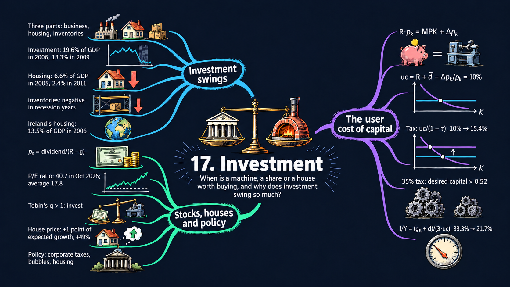




Learning goals
Investment links the present to the future: a firm that buys a machine today gives up money now for output later. One tool, the arbitrage equation, explains investment in machines, in stocks and in houses. By the end of this chapter you will be able to:
- use an arbitrage equation to compare two ways of investing the same money, and derive from it the user cost of capital, with and without a corporate income tax;
- derive the desired capital stock, where the marginal product of capital equals the user cost, and the investment rate it implies, step by step from a Cobb-Douglas production function;
- read the comparative statics of desired capital and the investment rate as elasticities, and rebuild Table 17.1 of corporate taxes and user costs for any year;
- derive the price of a stock as the present value of its dividends, \(\text{dividend}/(R-g)\), and use it to read the price-earnings ratio of the stock market, Tobin’s \(q\) and the price of a house;
- describe the components of private investment, in the U.S. and in 34 other countries, and how they move in recessions;
- write Python functions with default values, draw Plotly figures with sliders and buttons, reshape tables with
rename,meltandmerge, and repeat steps withforandwhileloops.
Model overview
Back on Islandia, Harbor Boatworks builds the island’s fishing boats. This year it has some cash to spare, and it faces a plain choice: leave the money in a savings account at a bank in town, or buy one more machine for its workshop, say a power saw that cuts planks. How many machines should the firm own, and how much should it spend on new ones each year? One idea answers both questions, and it also prices a share of Harbor Boatworks and an islander’s seaside cottage.
NoteThe big idea
The question. How much capital does a firm want to own, and how does that wish turn into a yearly flow of investment?
The answer in one sentence. By the arbitrage equation, a firm adds capital until the last unit earns its user cost: the bank’s interest plus wear and tear, minus any rise in its price.
What goes in and what comes out. We choose the interest rate, depreciation, the expected price change of capital, taxes and productivity. The model gives back the user cost, desired capital, the investment rate, and the prices of a share and a house.
Road map.
- Investment and the user cost of capital: the assumptions, the arbitrage equation and the user cost in solving the model, and what the model predicts.
- Taxes and the user cost: what a tax on Harbor Boatworks’ profits does to the cost of capital.
- From desired capital to investment: how many machines the firm wants, and what share of output it invests.
- The stock market: pricing a share: what a share of Harbor Boatworks is worth.
- Tobin’s q: the stock market and investment: how the share price tells the firm whether to invest.
- Housing: the arbitrage equation for a house: the price of a cottage bought with a mortgage.
- Model in code: every key result as a Python function, checked with numbers.
Notation. A bar over a letter marks a parameter that comes from outside the model, such as \(\bar{d}\) or \(\bar{A}\); Jones writes some given numbers, such as \(R\), \(\tau\) and \(L\), without a bar. All rates are decimals: \(R = 0.02\) means 2 percent a year.
| Symbol | Meaning | Type |
|---|---|---|
| \(K\), \(K^{\text{desired}}\) | the firm’s capital stock, and the stock it wants | endogenous |
| \(Y\), \(I_t\) | output, and investment in year \(t\) | endogenous |
| \(MPK\) | marginal product of capital: the extra output of one more unit of capital | endogenous |
| \(uc\) | user cost of capital: the yearly cost of using one more unit | endogenous |
| \(R\) | real interest rate: what a dollar earns in the bank for one year | parameter |
| \(\bar{d}\) | depreciation rate: the share of capital that wears out each year | parameter |
| \(p_k\), \(\Delta p_k/p_k\) | price of a new unit of capital, and its expected change in percent | parameters |
| \(\tau\) | tax rate (on profits, or on mortgage interest for a house) | parameter |
| \(\bar{A}\), \(L\), \(g_K\) | productivity, labor, and the growth rate of capital | parameters |
| \(p_s\), \(g\) | price of a share, and the growth rate of its dividend | endogenous, parameter |
| \(V\), \(q\) | stock market value of a firm, and Tobin’s \(q\) | endogenous |
| \(P^{\text{house}}\), \(\bar{x}\) | price of a house, and the down payment as a share of it | endogenous, parameter |
| \(\Delta x\) | the change \(x_{t+1} - x_t\) of any variable over one year | notation |
Investment and the user cost of capital
Assumptions
- Two uses of cash. Harbor Boatworks has money to spare. It can leave it in the bank for a year at the interest rate \(R\). Or it can buy one unit of capital, a power saw, at the price \(p_k\), use it in the workshop for a year, and sell it at the end of the year for \(p_{k,t+1} = p_k + \Delta p_k\).
- No risk. The firm knows in advance what each option pays, so only the size of the payoff matters.
- Diminishing returns. One more saw raises output by the marginal product of capital, \(MPK\). With the other inputs held fixed, \(MPK\) falls as the firm owns more capital (Chapter 4).
- Wear and tear. Like Islandia’s tools in Chapter 5, the saws wear out: a fraction \(\bar{d}\) of the capital is used up during the year.
- Profit maximization. The firm shifts money between the bank and the workshop until no shift can raise its profits.
The production model of Chapter 4 gave a first answer: add capital until \(MPK = R\). The argument below extends that rule to capital that wears out and changes in price.
Solving the model
Step 1: the arbitrage equation. Imagine the firm puts the same \(p_k\) dollars into each option for one year, and compare the payoffs. The bank pays interest on the whole sum. The saw pays its marginal product, plus whatever its price did during the year: a capital gain if the price went up, a capital loss if it went down. When the firm has chosen its capital stock well, neither option pays more than the other.
ImportantKey result: the arbitrage equation
\[\underbrace{R\cdot p_k}_{\text{deposit } p_k \text{ in the bank}} = \underbrace{MPK + \Delta p_k}_{\text{buy the machine, sell it after a year}} \tag{1}\]
Two safe uses of the same money must pay the same.
TipIn words: why the two sides end up equal
Suppose a new saw paid Harbor Boatworks more than the bank. Then the firm would buy another one. But each extra saw has less work to do than the one before, so \(MPK\) falls, and the firm keeps buying until the saw’s payoff has come down to the bank’s. If it paid less, the firm would hold fewer, busier saws. Either way it settles where equation (1) holds.
Step 2: returns per dollar. Choose the unit of capital so that one unit costs one dollar today, \(p_k = 1\), and divide both sides of (1) by \(p_k\). The left side is now just \(R\), and \(\Delta p_k/p_k\) is the capital gain in percent. Solve for \(MPK\):
\[R = MPK + \frac{\Delta p_k}{p_k} \quad\Longrightarrow\quad MPK = R - \frac{\Delta p_k}{p_k}.\]
If the price of capital never changes, \(\Delta p_k = 0\), we are back at the Chapter 4 rule, \(MPK = R\).
Step 3: depreciation. Wear and tear is a capital loss of its own kind: after a year in the workshop, only a share \(1-\bar{d}\) of the saw is left to sell. So we let \(p_k\) be the price of a new unit and write depreciation as its own term. One dollar of capital then returns \(MPK - \bar{d} + \Delta p_k/p_k\). Set this equal to \(R\), and move \(\bar{d}\) and the capital gain to the other side:
\[R = MPK - \bar{d} + \frac{\Delta p_k}{p_k} \quad\Longrightarrow\quad MPK = R + \bar{d} - \frac{\Delta p_k}{p_k}.\]
ImportantKey result: the user cost
\[MPK = \underbrace{R + \bar{d} - \frac{\Delta p_k}{p_k}}_{\text{user cost of capital, } uc} \tag{2}\]
We call \(uc\) the user cost of capital: what one more unit of capital costs to use for a year. It has three parts: the interest given up by not leaving the money in the bank (\(R\)), the part of the machine that wears out (\(\bar{d}\)), and, with a minus sign, any rise in the machine’s price, which the firm gets back when it sells.
Islandia in numbers. With this notebook’s baseline, \(R = 0.02\), \(\bar{d} = 0.08\) and a constant price of capital, \(uc = 0.02 + 0.08 - 0 = 0.10\). A saw must add at least 10 cents of output a year for every dollar it costs.
A machine is worth buying only if it earns the bank’s interest plus its own wear and tear, minus any rise in its price.
NoteCheck your understanding
1. Harbor Boatworks also uses design computers, whose price falls by 4 percent a year. With \(R = 0.02\) and \(\bar{d} = 0.08\), what is their user cost?
Answer
A falling price is a capital loss, \(\Delta p_k/p_k = -0.04\). Equation (2) gives \(uc = 0.02 + 0.08 + 0.04 = 0.14\), or 14 percent. Each dollar of computers must add 14 cents of output a year, not 10.
2. Suppose the last saw the firm bought adds more output than its user cost. Has the firm chosen its capital stock well?
Answer
No. One more saw would pay more than the same money in the bank, so the firm should buy it. Diminishing returns then bring \(MPK\) down to the user cost of equation (2).
What the model predicts
In Fig. 1, \(MPK\) is a curve that falls as capital rises, and the user cost is a flat line, because it does not depend on how many saws the firm owns. The firm buys capital up to the point where the two meet. Anything that raises the user cost lifts the flat line and moves that point to the left:
| A rise in … | changes the user cost by | Desired capital | Which line moves |
|---|---|---|---|
| interest rate \(R\) | \(+1\) point per point | falls | user-cost line up |
| depreciation rate \(\bar{d}\) | \(+1\) point per point | falls | user-cost line up |
| expected capital gain \(\Delta p_k/p_k\) | \(-1\) point per point | rises | user-cost line down |
| productivity \(\bar{A}\) | no change | rises | the \(MPK\) curve shifts up |
Equipment whose price keeps falling, such as computers, loses value every year on top of wearing out, so it is expensive to hold. A building on land that tends to gain value brings a capital gain, which lowers its user cost. So, for the same \(MPK\) curve, a firm holds fewer computers and more buildings.
Higher interest rates, faster wear and expected price falls all raise the user cost, and the firm wants fewer machines.
NoteCheck your understanding
1. The interest rate on Islandia rises from 2 to 3 percent, with \(\bar{d} = 0.08\) and no price change. What is the new user cost, and which way does Harbor Boatworks’ desired capital stock move?
Answer
By equation (2), \(uc = 0.03 + 0.08 = 0.11\). The flat line in Fig. 1 moves up, so it meets the falling \(MPK\) curve at a smaller capital stock: the firm wants fewer saws.
Taxes and the user cost
Assumptions
Keep every assumption above, and add a corporate income tax. The Islandia Treasury takes a share \(\tau\) of the extra income that each unit of capital produces, so Harbor Boatworks keeps \((1-\tau)MPK\). As in the textbook’s version, depreciation and capital gains are not taxed. One unit of new capital still costs one dollar, \(p_k = 1\).
Solving the model
Step 1: the arbitrage equation after tax. The money still costs \(R\). What a dollar of capital returns is now the marginal product after tax, minus depreciation, plus the capital gain:
\[\underbrace{R}_{\text{cost of the funds}} = \underbrace{(1-\tau)MPK - \bar{d} + \frac{\Delta p_k}{p_k}}_{\text{return on a dollar of capital}}.\]
Step 2: solve for the marginal product. Add \(\bar{d}\) to both sides and subtract the capital gain, so that only the taxed term is left on the right: \(R + \bar{d} - \Delta p_k/p_k = (1-\tau)MPK\). Divide both sides by \(1-\tau\):
\[MPK = \frac{R + \bar{d} - \Delta p_k/p_k}{1-\tau}.\]
ImportantKey result: the user cost with a corporate tax
\[MPK = \underbrace{\frac{R + \bar{d} - \Delta p_k/p_k}{1-\tau}}_{\text{user cost with the tax}} \tag{3}\]
The tax divides the user cost by \(1-\tau\).
Islandia in numbers. A tax of \(\tau = 0.35\) raises the baseline user cost from \(0.10\) to \(0.10/0.65 \approx 0.154\), about 15.4 percent.
TipIn words
The Islandia Treasury takes a slice of what every saw produces, but it pays no part of the saw’s costs. The interest, the wear and tear and the price change are just as before. So a saw must produce more before tax, by the factor \(1/(1-\tau)\), to leave Harbor Boatworks the same return after tax as the bank.
A tax on the profits of capital works like a higher price of using it: the bar each machine must clear goes up.
What the model predicts
- Direction. A higher tax rate always raises the user cost, so the firm wants less capital. In Fig. 2 the user-cost line shifts up and the firm climbs its \(MPK\) curve to a smaller capital stock.
- Size. Take logs of equation (3) (Appendix C.4): \(\ln uc = \ln(R + \bar{d} - \Delta p_k/p_k) - \ln(1-\tau)\). When the share the firm keeps, \(1-\tau\), falls by 1 percent, the user cost rises by 1 percent.
- The tax magnifies everything else. With the tax, each extra point of \(R\) or \(\bar{d}\) raises the user cost by \(1/(1-\tau)\) points: 1.54 points when \(\tau = 0.35\).
- Comparing countries. Suppose the user cost before tax is the same in every country. Then equation (3) gives each country’s user cost from a single known one: \(uc_i = uc_{\text{US}}\times(1-\tau_{\text{US}})/(1-\tau_i)\). With \(uc_{\text{US}} = 0.10\) and \(\tau_{\text{US}} = 0.21\), the user cost before tax is \(0.10\times0.79 = 0.079\). This is how we rebuild Table 17.1 in the key numbers after Fig. 2.
Corporate taxes raise the cost of capital, and they make it more sensitive to interest rates and depreciation.
NoteCheck your understanding
1. Use the before-tax user cost of 0.079 from Table 17.1. What is the user cost in a country whose corporate tax rate is 30 percent?
Answer
By equation (3), \(uc = 0.079/(1-0.30) = 0.079/0.70 \approx 0.113\), about 11.3 percent.
2. Why does a tax make the user cost react more strongly to a change in the interest rate?
Answer
In equation (3), the interest rate sits in the numerator, which is divided by \(1-\tau\). So each point of \(R\) adds \(1/(1-\tau)\) points to the user cost, more than one point whenever \(\tau > 0\).
From desired capital to investment
Assumptions
- Production. Harbor Boatworks (or Islandia as a whole) produces with the Cobb-Douglas function of Chapter 4, \(Y = \bar{A}K^{1/3}L^{2/3}\), with labor fixed at \(L\).
- Desired capital. The firm holds the capital stock at which \(MPK = uc\), with the user cost of equation (2), or of equation (3) when there is a tax.
- Capital accumulation. As in the Solow model, next year’s capital is this year’s investment plus the capital that has not worn out: \[K_{t+1} = I_t + (1-\bar{d})K_t.\]
- Growth. In the long run the capital stock grows at a rate \(g_K \equiv \Delta K_{t+1}/K_t\), which the growth models of Chapters 5 and 6 determine. Here we take it as given.
Our baseline. Besides \(R = 0.02\) and \(\bar{d} = 0.08\), we set \(\bar{A} = 0.3\) and \(L = 1\). These two values are our own choice. They make the desired capital stock exactly \(K = 1\) and output \(Y = 0.3\), so that Figs. 1 and 2 start from round numbers. For the investment rate we use an illustrative \(g_K = 0.02\).
Solving the model
Step 1: the marginal product of capital. \(MPK\) is the derivative of output with respect to capital, with labor held fixed (Appendix C.7). By the power rule, the exponent \(1/3\) moves to the front and drops by one, to \(1/3 - 1 = -2/3\):
\[MPK = \frac{\partial Y}{\partial K} = \frac{1}{3}\bar{A}K^{-2/3}L^{2/3}.\]
Two other ways of writing this are useful. First, \(\bar{A}K^{-2/3}L^{2/3} = \bar{A}K^{1/3}L^{2/3}/K = Y/K\), since dividing by \(K\) lowers its exponent by one. Second, \(K^{-2/3}L^{2/3} = (L/K)^{2/3}\), since two powers with the same exponent combine into one power of their ratio (Appendix C.3). Hence
\[MPK = \frac{1}{3}\cdot\frac{Y}{K} = \frac{1}{3}\cdot\bar{A}\left(\frac{L}{K}\right)^{2/3}.\]
The exponent on \(K\) is negative, so \(MPK\) falls as capital rises: diminishing returns. (In the textbook’s statement of this production function the exponent on labor is printed as \(1/2\). Constant returns to scale require \(2/3\), which is also the value the \(MPK\) formula uses.)
Step 2: the desired capital stock. Set the second form equal to the user cost and solve for \(K\). First multiply both sides by \(3/\bar{A}\):
\[\frac{1}{3}\bar{A}\left(\frac{L}{K}\right)^{2/3} = uc \quad\Longrightarrow\quad \left(\frac{L}{K}\right)^{2/3} = \frac{3\,uc}{\bar{A}}.\]
Then raise both sides to the power \(3/2\), because \(\left((L/K)^{2/3}\right)^{3/2} = L/K\), and flip both sides:
\[\frac{L}{K} = \left(\frac{3\,uc}{\bar{A}}\right)^{3/2} \quad\Longrightarrow\quad K = L\left(\frac{\bar{A}}{3\,uc}\right)^{3/2}.\]
Step 3: the capital-output ratio. Now set the first form equal to the user cost, \(\frac{1}{3}\,Y/K = uc\), and multiply both sides by 3 to get \(Y/K = 3\cdot uc\).
ImportantKey result: the marginal product and the desired capital stock
\[MPK = \frac{1}{3}\cdot\frac{Y}{K} = \frac{1}{3}\cdot\bar{A}\left(\frac{L}{K}\right)^{2/3} \tag{4}\]
\[K^{\text{desired}} = L\left(\frac{\bar{A}}{3\,uc}\right)^{3/2} \tag{5}\]
\[\frac{Y}{K} = 3\cdot uc \tag{6}\]
Islandia in numbers. In the baseline, \(\bar{A}/(3\,uc) = 0.3/0.3 = 1\), so \(K^{\text{desired}} = 1\). Output is \(3\times0.10 = 0.30\) per unit of capital, so the firm holds capital worth \(1/0.3 \approx 3.3\) years of output.
TipIn words: what productivity does and does not change
If Harbor Boatworks’ workers became more productive, every saw would earn more, and the firm would want more saws (equation 5). But equation (6) holds for any \(\bar{A}\) and \(L\). Output and capital rise together, so the ratio of output to capital stays where the user cost puts it.
Step 4: the investment that reaches the desired stock. In the accumulation equation, put the firm’s current capital \(K_t\) on the right and its desired capital in place of \(K_{t+1}\), then solve for investment:
\[I_t = K^{\text{desired}} - (1-\bar{d})K_t.\]
A firm with \(K_t = 0.5\) that wants \(K = 1\) next year must invest \(1 - 0.92\times0.5 = 0.54\): 0.50 to grow and 0.04 to replace the capital that wears out. If \(K^{\text{desired}}\) is below \((1-\bar{d})K_t\), the formula gives a negative number. The firm then stops investing and lets depreciation shrink its capital, or sells some of it.
Step 5: the investment rate. Subtract \(K_t\) from both sides of the accumulation equation to write it as a change, and divide by \(K_t\):
\[\Delta K_{t+1} = I_t - \bar{d}K_t \quad\Longrightarrow\quad \frac{\Delta K_{t+1}}{K_t} = \frac{I_t}{K_t} - \bar{d}.\]
Write \(I_t/K_t\) as the product \((I_t/Y_t)\cdot(Y_t/K_t)\). The \(Y_t\) cancels, so the value does not change, but the investment rate \(I_t/Y_t\) now shows up:
\[g_K = \frac{I_t}{Y_t}\cdot\frac{Y_t}{K_t} - \bar{d}.\]
Replace \(Y_t/K_t\) by \(3\cdot uc\) from equation (6), add \(\bar{d}\) to both sides, and divide by \(3\cdot uc\).
ImportantKey result: the investment rate
\[\frac{I_t}{Y_t} = \frac{g_K + \bar{d}}{3\cdot uc} \tag{7}\]
Islandia in numbers. With \(g_K = 0.02\), \(\bar{d} = 0.08\) and \(uc = 0.10\), the investment rate is \(0.10/0.30 \approx 33\) percent. With the 35 percent tax, \(uc \approx 0.154\) and the rate falls to about 21.7 percent.
TipIn words
The numerator is the new capital needed for each unit Harbor Boatworks already owns: enough to grow by \(g_K\) and to replace what wore out. The denominator turns “per unit of capital” into “per unit of output”. When the user cost is high, the firm holds little capital for each boat it builds (equation 6), so keeping that small stock growing takes only a small share of output.
The user cost sets how much capital a firm wants, and the investment rate is what it takes to keep that capital growing.
NoteCheck your understanding
1. The interest rate rises to \(R = 0.03\), so \(uc = 0.11\), with \(\bar{A} = 0.3\), \(L = 1\) and \(g_K = 0.02\). What are Harbor Boatworks’ desired capital and Islandia’s investment rate?
Answer
Now \(3\,uc = 0.33\). Equation (5) gives \(K^{\text{desired}} = (0.3/0.33)^{3/2} \approx 0.87\), down from 1. Equation (7) gives \(I/Y = 0.10/0.33 \approx 0.303\), about 30.3 percent instead of 33 percent.
2. After the 35 percent tax, the firm wants \(K \approx 0.52\) but owns \(K = 1\). If it stops investing, how many years does depreciation take to bring its capital below the new target?
Answer
With \(I_t = 0\), the accumulation equation gives \(K_{t+1} = 0.92\,K_t\). After \(n\) years capital is \(0.92^n\), and \(0.92^n < 0.52\) first holds at \(n = 8\) (since \(0.92^8 \approx 0.513\)). So it takes 8 years without any investment, as the key numbers after Fig. 2 confirm.
What the model predicts
Take logs of equations (5) and (7) (Appendix C.4):
\[\ln K^{\text{desired}} = \ln L + \tfrac{3}{2}\ln\bar{A} - \tfrac{3}{2}\ln 3 - \tfrac{3}{2}\ln uc, \qquad \ln\frac{I}{Y} = \ln(g_K + \bar{d}) - \ln 3 - \ln uc.\]
Each coefficient is an elasticity:
| A 1% rise in … | changes \(K^{\text{desired}}\) by | changes \(I/Y\) by | Which curve moves |
|---|---|---|---|
| user cost \(uc\) (from \(R\), \(\bar{d}\), a capital loss or \(\tau\)) | \(-1.5\%\) | \(-1\%\) | user-cost line up |
| productivity \(\bar{A}\) | \(+1.5\%\) | \(0\) | \(MPK\) curve up |
| labor \(L\) | \(+1\%\) | \(0\) | \(MPK\) curve up |
| the after-tax share \(1-\tau\) | \(+1.5\%\) | \(+1\%\) | user-cost line down |
- Capital reacts more than one for one. Desired capital is proportional to \(uc^{-3/2}\), so the 35 percent tax shrinks it by the factor \(0.65^{3/2} \approx 0.52\), nearly in half. The reason is the long, flat tail of the \(MPK\) curve: when returns fall off slowly, a small rise in the return the firm demands removes a lot of capital.
- Productivity and labor raise capital, not the investment rate. They push the \(MPK\) curve up, so the firm wants more capital. But they do not appear in equation (7): output grows in proportion, and \(I/Y\) stays put.
- Depreciation pulls two ways. A higher \(\bar{d}\) adds replacement investment to the numerator of (7), and it also raises the user cost in the denominator. Write \(uc = R + \bar{d} - \Delta p_k/p_k\) and take the derivative: the net effect on \(I/Y\) has the sign of \(R - \Delta p_k/p_k - g_K\). In our baseline \(R = g_K = 0.02\) and there is no capital gain, so the two effects cancel exactly and \(I/Y = 1/3\), capital’s exponent, for any \(\bar{d}\).
- A theory of the saving rate. The Solow model of Chapter 5 took the investment rate \(\bar{s}\) as given. Equation (7) explains it: taxes, interest rates and depreciation move it through the user cost. Add the growth models (which set \(g_K\)) and the Euler equation of Chapter 16 (which sets the long-run interest rate), and equations (6) and (7) close a long-run model of a closed economy: its capital-output ratio, its investment rate, and so the share of GDP that is consumed.
- Reaching the target takes time. Installing new capital is costly and disrupts production, so real firms approach \(K^{\text{desired}}\) over several years, not in one jump.
Desired capital is very sensitive to the user cost, while the investment rate depends only on the user cost, growth and depreciation.
NoteCheck your understanding
1. Keep \(R = g_K = 0.02\) and no capital gain, but let depreciation rise from 0.08 to 0.12. What is the new investment rate?
Answer
The user cost becomes \(0.02 + 0.12 = 0.14\), and equation (7) gives \(I/Y = (0.02 + 0.12)/(3\times0.14) = 0.14/0.42 \approx 0.333\). The rate does not move: more replacement investment is exactly offset by a smaller capital stock per unit of output.
Tobin’s q: the stock market and investment
Definitions
James Tobin compared two values of the same firm. One is what the stock market says the firm is worth, \(V\): the present value of all its future profits. The other is what it would cost to buy all of its capital new, \(p_kK\).
ImportantKey result: Tobin’s q
\[q = \frac{V}{p_kK} = \frac{\text{stock market value of the firm}}{\text{replacement cost of its capital}} \tag{11}\]
Tobin’s \(q\) compares what the market pays for Harbor Boatworks with the cost of rebuilding its workshop.
Solving the model
Step 1: the value of a firm that owns only capital. Take a firm with the Cobb-Douglas technology above, \(p_k = 1\), no taxes and a constant price of capital. Capital is paid its marginal product, so the firm’s capital income is \(MPK\cdot K\), exactly a third of output with the exponent \(1/3\). Each year it spends \(\bar{d}K\) to replace the capital that wore out, which keeps \(K\) constant, and it pays the rest to its shareholders. So its dividend is constant, \((MPK - \bar{d})K\), and equation (9) with \(g = 0\) gives the firm’s value:
\[V = \frac{(MPK - \bar{d})K}{R}.\]
Step 2: divide by the value of capital. With \(p_k = 1\), the denominator of equation (11) is just \(K\), which cancels.
ImportantKey result: q for a firm that owns only capital
\[q = \frac{MPK - \bar{d}}{R} \tag{12}\]
Islandia in numbers. At its desired capital, \(K = 1\), Harbor Boatworks has \(MPK = 0.10\) and \(q = (0.10 - 0.08)/0.02 = 1\). With only \(K = 0.5\), it has \(MPK \approx 0.159\) and \(q \approx 3.9\).
Step 3: the link to the user cost. \(q = 1\) exactly when \(MPK - \bar{d} = R\), that is, when \(MPK = R + \bar{d}\): the user cost of equation (2) without a capital gain. So a \(q\) above 1 is the stock market’s way of saying that \(MPK\) is above the user cost:
\[q > 1 \iff MPK > uc \iff \text{the firm should invest}.\]
TipIn words
When \(q > 1\), Harbor Boatworks could sell new shares, spend the money on saws, and be worth more than the saws cost: investing creates value for its owners. When \(q < 1\), the firm is worth less than its machines, and its owners would gain by selling some of them.
Tobin’s q reads the firm’s investment signal off the stock market: above one, buy capital; below one, shrink.
What the model predicts
- \(q\) near 1. If adjusting the capital stock cost nothing, firms would keep \(MPK = uc\) at every moment, so \(q\) would always be 1. When installing capital is slow and costly (a production line must stop, a new plant must be built), firms close the gap gradually, and \(q\) can stay above or below 1 for a while.
- \(q\) predicts investment. Firms with a high \(q\) should invest, and firms with a low \(q\) should shrink.
- In the data, \(q\) is often well above 1, because firms own assets that are not counted in \(K\): brand names, patents and know-how, which the stock market values too.
- Financial frictions. Studies of many firms find that tax changes move investment through \(q\) and the user cost, as the theory predicts. But a firm’s own cash flow, and how easily it can borrow from banks or raise money in financial markets, also matter, and the simple model leaves them out.
In practice q drifts away from one, because capital takes time to install and markets value more than machines.
NoteCheck your understanding
1. Harbor Boatworks has overbuilt and owns \(K = 1.2\). With the baseline \(\bar{A} = 0.3\), \(L = 1\), \(R = 0.02\) and \(\bar{d} = 0.08\), what are its \(MPK\) and its \(q\)? What should it do?
Answer
Equation (4) gives \(MPK = 0.1\times(1/1.2)^{2/3} \approx 0.089\). Equation (12) gives \(q = (0.089 - 0.08)/0.02 \approx 0.43\). Since \(q < 1\), its \(MPK\) is below the user cost of 0.10: it should stop investing and let its capital shrink toward \(K = 1\).
Housing: the arbitrage equation for a house
Assumptions
- The investor. An islander can keep her down payment in the bank at the interest rate \(R\), or use it to buy a seaside cottage at the price \(P^{\text{house}}\), rent it out for a year, and sell it.
- Leverage. The down payment is a share \(\bar{x}\) of the price. She borrows the rest, \((1-\bar{x})P^{\text{house}}\), with a mortgage at the rate \(R\). The leverage ratio, the price of the house per dollar of her own money, is \(1/\bar{x}\).
- Taxes. Mortgage interest is deductible at the tax rate \(\tau\), so each dollar of interest costs her only \(1-\tau\) dollars.
- The house. It earns a rent, wears out at the rate \(\bar{d}\) of its value, and its price changes by \(\Delta P^{\text{house}}\) during the year. There is no risk, and buying or selling costs nothing.
Solving the model
Step 1: the arbitrage equation. The bank pays \(R\) on the down payment. The cottage pays the rent, minus depreciation, plus the capital gain, minus the interest on the mortgage after tax:
\[R\cdot\bar{x}P^{\text{house}} = \text{rent} - \bar{d}P^{\text{house}} + \Delta P^{\text{house}} - R(1-\tau)(1-\bar{x})P^{\text{house}}.\]
Step 2: divide by the price. Every term except the rent contains \(P^{\text{house}}\):
\[R\bar{x} = \frac{\text{rent}}{P^{\text{house}}} - \bar{d} + \frac{\Delta P^{\text{house}}}{P^{\text{house}}} - (1-\tau)R(1-\bar{x}).\]
Step 3: collect the interest terms. Move every term except the rent ratio to the left. Expand \((1-\tau)R(1-\bar{x}) = (1-\tau)R - (1-\tau)R\bar{x}\). The two terms in \(R\bar{x}\) then combine into \(R\bar{x} - (1-\tau)R\bar{x} = \tau\bar{x}R\):
\[\frac{\text{rent}}{P^{\text{house}}} = \tau\bar{x}R + (1-\tau)R + \bar{d} - \frac{\Delta P^{\text{house}}}{P^{\text{house}}}.\]
Step 4: solve for the price. Flip both sides and multiply by the rent.
ImportantKey result: the price of a house
\[P^{\text{house}} = \frac{\text{rent}}{\tau\bar{x}R + (1-\tau)R + \bar{d} - \Delta P^{\text{house}}/P^{\text{house}}} \tag{13}\]
The denominator is the user cost of a house.
Islandia in numbers. With the values of the house price key numbers, a rent of 6,000 dollars a year, \(R = 0.04\), \(\bar{d} = 0.02\), \(\tau = 0.3\), \(\bar{x} = 0.2\) and expected price growth of 0.02, the denominator is \(0.0024 + 0.028 + 0.02 - 0.02 = 0.0304\), and the cottage is worth \(6000/0.0304\), about 197,000 dollars.
TipIn words
The cottage’s user cost works like the saw’s in equation (2): the interest on the down payment and on the loan (made cheaper by the tax deduction), plus depreciation, minus the price gain she expects. The price is the present value of the rents, discounted at that user cost. Without the tax, \(\tau = 0\), the denominator is just \(R + \bar{d} - \Delta P^{\text{house}}/P^{\text{house}}\), the user cost of any capital good.
A house is priced like any capital good: its rent divided by its user cost.
What the model predicts
The price rises when the denominator of (13) falls. The derivative of the denominator with respect to each parameter gives:
| A rise in … | changes the denominator by | House price |
|---|---|---|
| rent | no change (the numerator rises) | rises in proportion |
| interest rate \(R\) | \(\tau\bar{x} + 1 - \tau\) per point | falls |
| depreciation \(\bar{d}\) | \(+1\) per point | falls |
| expected price growth \(\Delta P/P\) | \(-1\) per point | rises |
| down payment share \(\bar{x}\) | \(+\tau R\) per unit | falls |
| tax rate \(\tau\) | \(-(1-\bar{x})R\) per unit | rises |
- Leverage matters, but only a little. A smaller down payment (more leverage) raises the price, but its effect is scaled by \(\tau R\), a small number: with \(\tau = 0.3\) and \(R = 0.04\) it is 0.012, so cutting \(\bar{x}\) by 10 points lowers the denominator by only 0.0012.
- Expectations matter a lot. One more point of expected price growth lowers the denominator by a full 0.01, about eight times the effect of that 10-point cut in the down payment. If rising prices lead people to expect more rises, the price can keep climbing on its own: a housing bubble that feeds itself. As with shares, such a bubble is hard to tell apart from a real change in rents, interest rates or credit.
- Inventories, the last part of investment, follow the same logic of comparing returns, but the chapter treats them only in words. Firms keep goods moving through production and stocked on the shelf so as not to run out, and both motives make inventory investment rise in booms and fall in recessions (Fig. 4).
Easier credit nudges house prices up; expected price gains can push them up by far more.
NoteCheck your understanding
1. Starting from the cottage’s baseline, the down payment falls from 20 to 10 percent. By how much does the price change?
Answer
The term \(\tau\bar{x}R\) falls from 0.0024 to 0.0012, so the denominator of equation (13) falls from 0.0304 to 0.0292. The price rises by the factor \(0.0304/0.0292\), about 4.1 percent.
2. Instead, islanders come to expect the price to grow 3 percent a year rather than 2. By how much does the price change now?
Answer
The denominator falls by a full point of expected growth, from 0.0304 to 0.0204. The price rises by the factor \(0.0304/0.0204\), about 49 percent, to roughly 294,000 dollars.
NoteRecap
- One idea, many assets: two safe uses of the same money must pay the same return. This arbitrage equation prices machines, shares and houses alike.
- The user cost of capital is \(R + \bar{d} - \Delta p_k/p_k\), and a firm adds capital until \(MPK\) falls to it (Fig. 1).
- A corporate tax divides the user cost by \(1-\tau\); desired capital falls with \(uc^{-3/2}\) and the investment rate with \(1/uc\) (Fig. 2).
- A share is worth its discounted dividends, \(\text{dividend}/(R-g)\), so the P/E ratio is very sensitive to expected growth, and bubbles are hard to spot (Fig. 3).
- Tobin’s \(q\) above 1 tells a firm to invest; for houses, expected price gains matter far more than leverage (key numbers).
- In the data, investment, and above all housing and inventories, falls sharply in recessions (Fig. 4, in Investment in the data).
Model in code
Now we turn the Key results into Python. The section has four parts: the setup (folded, because it is the same in every chapter), the model as functions, numerical checks of the Key results, and the drawing tools that Figs. 1 and 2 use (folded too). Run its cells once, in order. Every later section of the notebook reuses them.
Setup
Run the setup cells once, before anything else. They load the Python libraries, give every chart the same look, store the address of the chapter’s data and define a helper that only the book website needs. You can use the notebook without reading them; open the box if you are curious.
NoteShow the setup code
The first cell loads the libraries and sets the look of the charts. Its comments explain each step.
The website cannot run Python, so each interactive figure also gets a version with a precomputed slider. The next helper builds those versions. Run it and move on.
# @title Helper for the website versions (run this cell; you do not need to read it)
def slider_figure(make_figure, name, values, start, label=None):
    """Join precomputed versions of a figure with one slider (the website cannot run Python).

    Arguments
        make_figure : the function that draws the figure, e.g. desired_capital_diagram
        name        : the argument the slider moves, e.g. "R"
        values      : the values of that argument to precompute
        start       : the value shown first
        label       : the slider's label (the argument name if None)
    Returns
        one Plotly figure with all versions and a slider that shows one at a time
    """
    # Step 1: draw the figure once for every value
    figures = [make_figure(**{name: v}) for v in values]
    first = values.index(start)
    # Step 2: copy every curve into one figure; only the start value's are visible
    fig = go.Figure(layout=figures[first].layout)
    owner = []                          # which precomputed figure each trace is from
    for i, f in enumerate(figures):
        for trace in f.data:
            trace.visible = (i == first)
            fig.add_trace(trace)
            owner.append(i)
    # Step 3: one slider step per value: its curves, title, labels and shapes
    steps = []
    for i, f in enumerate(figures):
        layout = {"title": f.layout.title.to_plotly_json(),
                  "annotations": [a.to_plotly_json() for a in f.layout.annotations],
                  "shapes": [s.to_plotly_json() for s in f.layout.shapes]}
        visible = [o == i for o in owner]
        steps.append(dict(method="update", label=str(values[i]), args=[{"visible": visible}, layout]))
    fig.update_layout(sliders=[dict(active=first, steps=steps, pad=dict(t=60),
                                    currentvalue=dict(prefix=(label or name) + " = "))])
    return fig
The model as functions
Four Key results describe Harbor Boatworks’ choice: the user cost, equations (2) and (3); the marginal product of capital, equation (4); desired capital, equation (5); and the investment rate, equation (7). We write each one as a Python function: a named recipe that takes inputs and gives back a result. Two constants come first, an illustrative productivity and labor force, chosen so that the baseline desired capital stock is 1.
# The constants and the four functions of the firm's choice of capital.
# Names in capitals, such as `A_BAR`, are constants that we set once and reuse.
# illustrative productivity A-bar and labor L: the baseline desired capital is K = 1
A_BAR, L_BAR = 0.3, 1.0


# `def` creates a function. Its inputs are the arguments in parentheses.
# `gpk=0.0` gives gpk a default value, used whenever we do not pass one.
# The text in triple quotes describes the function.
def user_cost(R, d, gpk=0.0, tau=0.0):
    """User cost of capital, uc.

    Equation (2), or (3) with a tax:  uc = (R + d - gpk) / (1 - tau)

    Arguments
        R   : real interest rate
        d   : depreciation rate, d-bar
        gpk : expected capital gain, the change in p_k over p_k (0 unless we pass one)
        tau : corporate tax rate (0 in the basic model)
    Returns
        the user cost of capital, uc
    """
    # `return` gives back the result: interest plus wear and tear minus the
    # capital gain, divided by the share of profits the firm keeps
    return (R + d - gpk) / (1 - tau)


def mpk(K, A=A_BAR, L=L_BAR):
    """Marginal product of capital, MPK.

    Equation (4):  MPK = (1/3) A (L/K)^(2/3)

    Arguments
        K : capital
        A : productivity, A-bar
        L : labor
    Returns
        the marginal product of capital, MPK
    """
    # `**` means "to the power of"; K may also be a whole array of capital stocks
    return A / 3 * (L / K) ** (2 / 3)


def desired_capital(uc, A=A_BAR, L=L_BAR):
    """Desired capital stock, where MPK equals the user cost.

    Equation (5):  K-desired = L (A / (3 uc))^(3/2)

    Arguments
        uc : user cost of capital
        A  : productivity, A-bar
        L  : labor
    Returns
        the desired capital stock, K-desired
    """
    # equation (4) set equal to uc and solved for K
    return L * (A / (3 * uc)) ** (3 / 2)


def investment_rate(uc, g_K=0.02, d=0.08):
    """Investment rate of a firm that keeps its desired capital, I/Y.

    Equation (7):  I/Y = (g_K + d) / (3 uc)

    Arguments
        uc  : user cost of capital
        g_K : growth rate of capital
        d   : depreciation rate, d-bar
    Returns
        the investment rate, I/Y
    """
    # new capital (g_K) plus replacement (d), divided by Y/K = 3 uc, equation (6)
    return (g_K + d) / (3 * uc)
The same arbitrage idea prices a share of Harbor Boatworks and the firm itself. Three more functions write the price of a share, equation (9), its price-earnings ratio, equation (10), and Tobin’s \(q\), equation (12).
def stock_price(dividend, R, g=0.0):
    """Price of a share, p_s: the present value of its dividends.

    Equation (9):  p_s = dividend / (R - g)

    Arguments
        dividend : this year's dividend
        R        : real interest rate
        g        : growth rate of the dividend (0 unless we pass one)
    Returns
        the price of the share, p_s
    """
    # the dividend, discounted at the interest rate less the dividend's growth
    return dividend / (R - g)


def pe_ratio(payout, R, g):
    """Price-earnings ratio of a share.

    Equation (10):  p_s / earnings = (dividend / earnings) / (R - g)

    Arguments
        payout : the payout ratio, dividend / earnings
        R      : real interest rate
        g      : growth rate of the dividend
    Returns
        the price-earnings ratio, p_s / earnings
    """
    # equation (9) divided by earnings
    return payout / (R - g)


def tobin_q(K, R=0.02, d=0.08, A=A_BAR):
    """Tobin's q of a firm that owns only capital.

    Equation (12):  q = (MPK - d) / R

    Arguments
        K : the firm's capital
        R : real interest rate
        d : depreciation rate, d-bar
        A : productivity, A-bar
    Returns
        Tobin's q: the market value of the firm over the cost of its capital
    """
    # the return per unit of capital net of wear and tear, priced as a share with g = 0
    return (mpk(K, A) - d) / R
Checking the key results
The formulas came from algebra. Now we check them with numbers, one Key result at a time, using the baseline values \(R = 0.02\) and \(\bar{d} = 0.08\).
Check 1: the user cost and the arbitrage equation. At the desired capital stock, a dollar in capital must earn exactly what a dollar in the bank earns, with and without the tax.
# Check 1: the user cost without and with a 35% tax, and the arbitrage equation
# Step 1: the user cost, equations (2) and (3), and desired capital, equation (5)
uc_base = user_cost(R=0.02, d=0.08)
uc_tax = user_cost(R=0.02, d=0.08, tau=0.35)
K_base, K_tax = desired_capital(uc_base), desired_capital(uc_tax)

# Step 2: show the user costs. An f-string, f"... {value:.1%}", puts a value into
# the text; ":.1%" shows a share as a percentage with one decimal (0.1 is 10.0%).
print(f"User cost, no tax (equation 2):       {uc_base:.1%}")
print(f"User cost, 35% tax (equation 3):      {uc_tax:.1%}")
# Step 3: at desired capital, the bank and the machine pay the same (":.4f" shows
# four decimals); with the tax, the firm keeps only (1 - tau) of MPK
print(f"No tax:  bank pays R = 0.0200, capital pays MPK - d = {mpk(K_base) - 0.08:.4f}")
print(f"Tax:     bank pays R = 0.0200, capital pays (1 - tau) MPK - d = {(1 - 0.35) * mpk(K_tax) - 0.08:.4f}")
# Step 4: a capital gain lowers the user cost, a capital loss raises it
print(f"A capital gain of 2%: user cost {user_cost(0.02, 0.08, gpk=0.02):.1%}; a loss of 4%: {user_cost(0.02, 0.08, gpk=-0.04):.1%}")
User cost, no tax (equation 2): 10.0%
User cost, 35% tax (equation 3): 15.4%
No tax: bank pays R = 0.0200, capital pays MPK - d = 0.0200
Tax: bank pays R = 0.0200, capital pays (1 - tau) MPK - d = 0.0200
A capital gain of 2%: user cost 8.0%; a loss of 4%: 14.0%Check 2: desired capital, the capital-output ratio and the elasticity. Equation (5) must give a capital stock at which \(MPK\) equals the user cost, and there \(Y/K\) must equal \(3\cdot uc\) (equation 6). Raising the user cost by 1 percent should lower desired capital by about 1.5 percent.
# Check 2: desired capital, the output-capital ratio and the elasticity -3/2
# Step 1: output at desired capital, Y = A K^(1/3) L^(2/3)
Y_base = A_BAR * K_base ** (1 / 3) * L_BAR ** (2 / 3)
# Step 2: MPK equals uc there (equation 5), and Y/K equals 3 uc (equation 6)
print(f"Desired capital K = {K_base:.3f}, MPK there = {mpk(K_base):.4f}, user cost = {uc_base:.4f}")
print(f"Y/K = {Y_base / K_base:.4f}   and   3 x uc = {3 * uc_base:.4f}")
# Step 3: desired capital with a 1% higher user cost; ":+.3f" also shows the sign
change_K = desired_capital(uc_base * 1.01) / K_base - 1
print(f"1% higher user cost: desired capital changes by {100 * change_K:+.3f}%   (elasticity -1.5)")
# Step 4: a 35% tax multiplies desired capital by (1 - tau)^(3/2)
print(f"35% tax: K falls by the factor {K_tax / K_base:.4f}   and   0.65^(3/2) = {0.65 ** 1.5:.4f}")
Desired capital K = 1.000, MPK there = 0.1000, user cost = 0.1000
Y/K = 0.3000 and 3 x uc = 0.3000
1% higher user cost: desired capital changes by -1.481% (elasticity -1.5)
35% tax: K falls by the factor 0.5240 and 0.65^(3/2) = 0.5240Check 3: the investment rate, two ways. Let a firm hold its desired capital and grow it at \(g_K = 2\) percent. We compute the investment it needs from the accumulation equation, divide by output, and compare with equation (7).
# Check 3: the investment rate from the accumulation equation and from equation (7).
# `for tau in [0.0, 0.35]` runs the indented lines once for each tax rate in the list.
for tau in [0.0, 0.35]:
    # Step 1: the firm holds its desired capital at this tax rate
    uc = user_cost(0.02, 0.08, tau=tau)
    K_now = desired_capital(uc)
    # Step 2: the investment that grows capital by 2%, and output (L = 1)
    K_next = 1.02 * K_now                          # capital grows at g_K = 2 percent
    # accumulation equation K_next = I + (1 - d) K_now, solved for investment
    I = K_next - (1 - 0.08) * K_now
    Y = A_BAR * K_now ** (1 / 3)
    # Step 3: compare I/Y with equation (7)
    print(f"tau = {tau:.2f}: I/Y = {I / Y:.4f} (accumulation), {investment_rate(uc):.4f} (equation 7)")
tau = 0.00: I/Y = 0.3333 (accumulation), 0.3333 (equation 7)
tau = 0.35: I/Y = 0.2167 (accumulation), 0.2167 (equation 7)Equation (7) also says that, with \(R = g_K\) and no capital gain, depreciation does not change the investment rate.
# The investment rate of equation (7) for three depreciation rates, with R = g_K = 2%
for d in [0.05, 0.08, 0.12]:
    print(f"d = {d:.2f}: I/Y = {investment_rate(user_cost(0.02, d), g_K=0.02, d=d):.4f}")
d = 0.05: I/Y = 0.3333
d = 0.08: I/Y = 0.3333
d = 0.12: I/Y = 0.3333Check 4: the stock price is a present value. We add up the discounted dividends of the next 2,000 years, one year at a time, and compare the sum with equation (9). Then we confirm that the arbitrage equation makes the price grow at the rate \(g\).
# Check 4: the price of a share as the sum of its discounted dividends
# Step 1: the first dividend (dollars), the interest rate and the dividend's growth
D, R, g = 3.0, 0.05, 0.02
pv = 0.0                                           # the running total starts at zero

# Step 2: add up 2,000 years of dividends. `range(1, 2001)` counts 1, 2, ..., 2000,
# and `pv = pv + ...` adds one more term to the running total each year.
for t in range(1, 2001):
    # the dividend of year t, discounted to today
    pv = pv + D * (1 + g) ** (t - 1) / (1 + R) ** t
print(f"Sum of discounted dividends: {pv:.4f}   equation (9): {stock_price(D, R, g):.4f}")
print(f"No growth: {stock_price(D, R):.2f} dollars")

# Step 3: next year's price from the arbitrage equation, R p = dividend + change in p
p_now = stock_price(D, R, g)
p_next = (1 + R) * p_now - D
print(f"Price growth implied by arbitrage: {p_next / p_now - 1:.4f}   dividend growth g = {g:.4f}")
# Step 4: the P/E ratio of equation (10) when half of earnings is paid out
print(f"Model P/E ratio with a payout of 0.5: {pe_ratio(0.5, R, g):.1f}")
Sum of discounted dividends: 100.0000 equation (9): 100.0000
No growth: 60.00 dollars
Price growth implied by arbitrage: 0.0200 dividend growth g = 0.0200
Model P/E ratio with a payout of 0.5: 16.7Check 5: Tobin’s \(q\). A firm at its desired capital should have \(q = 1\), and its market value from equation (9) should equal its capital. A firm below its desired capital should have \(q > 1\), and one above it \(q < 1\).
# Check 5: Tobin's q, from the firm's market value and from equation (12),
# for a firm below, at and above its desired capital of 1
for K_firm in [0.5, 1.0, 1.2]:
    # the dividend (MPK - d) K, priced with equation (9) and g = 0
    V = (mpk(K_firm) - 0.08) * K_firm / 0.02
    print(f"K = {K_firm:.1f}: MPK = {mpk(K_firm):.4f}, V = {V:.3f}, q = V/K = {V / K_firm:.3f}, "
          f"equation (12): {tobin_q(K_firm):.3f}")
K = 0.5: MPK = 0.1587, V = 1.969, q = V/K = 3.937, equation (12): 3.937
K = 1.0: MPK = 0.1000, V = 1.000, q = V/K = 1.000, equation (12): 1.000
K = 1.2: MPK = 0.0886, V = 0.513, q = V/K = 0.428, equation (12): 0.428Check 6: the house price. We compute the price from equation (13), with the numbers used later in the notebook (a rent of 6,000 dollars a year, \(R = 0.04\), \(\bar{d} = 0.02\), \(\tau = 0.3\), \(\bar{x} = 0.2\), expected price growth of 2 percent). Then we put that price back into both sides of the arbitrage equation of step 1: they must match.
# Check 6: the cottage's price, equation (13), and both sides of the arbitrage equation
# Step 1: rent (dollars a year), R, d-bar, tau, x-bar and expected price growth
rent, R, d, tau, x, gp = 6000, 0.04, 0.02, 0.3, 0.2, 0.02
P = rent / (tau * x * R + (1 - tau) * R + d - gp)  # equation (13)
# Step 2: the return from keeping the down payment in the bank
bank = R * x * P
# the return from buying the house: rent, minus wear and tear, plus the price
# gain, minus the after-tax interest on the mortgage
house = rent - d * P + gp * P - R * (1 - tau) * (1 - x) * P
# Step 3: show them; ":,.0f" adds thousands separators and shows no decimals
print(f"House price: {P:,.0f} dollars")
print(f"Bank: {bank:,.2f} dollars   House: {house:,.2f} dollars")
House price: 197,368 dollars
Bank: 1,578.95 dollars House: 1,578.95 dollarsDrawing tools
Figs. 1 and 2 are the same kind of diagram, so we write its drawing steps once, as six small tools. Run them and move on, or open the box to see how they work.
NoteShow the drawing tools
capital_figure starts a diagram with fixed axes, so that you can see the curves move. Every line carries its name on the plot, its equation or its value, and add_label leaves a name out when another one already sits close by, so that two names never overlap.
# @title Drawing tools: an empty diagram, and line names that never overlap
# the fixed axes of Figs. 1 and 2
K_RANGE, RETURN_RANGE = [0, 3], [0, 0.4]


def capital_figure(title):
    """An empty diagram: capital across, the return per unit of capital (percent) up.

    Arguments
        title : the chart's title
    Returns
        an empty Plotly figure with the fixed axes of Figs. 1 and 2
    """
    # `go.Figure()` starts an empty chart; the other tools add its lines
    fig = go.Figure()
    # fixed axes and no legend: every line carries its name on the plot
    fig.update_layout(title=title, showlegend=False,
                      xaxis=dict(title="Capital, K", range=K_RANGE, tickvals=[0.5, 1, 1.5, 2, 2.5, 3],
                                 zeroline=False),
                      yaxis=dict(title="Return per unit of capital", range=RETURN_RANGE,
                                 tickvals=[0, 0.1, 0.2, 0.3, 0.4], tickformat=".0%", zeroline=False))
    return fig


def add_label(fig, x, y, text, color, xanchor="left"):
    """Write a line's name at (x, y), unless another name already sits within 2 points of it.

    Arguments
        fig     : the figure to write on
        x, y    : where the name goes
        text    : the name
        color   : its color, e.g. BLUE
        xanchor : "left" or "right": which end of the name sits at x
    """
    # Step 1: a `for` loop over `fig.layout.annotations` looks at every name already
    # written (`abs` is the absolute value). If one is close, a bare `return` leaves
    # the function early, without writing this name.
    for old in fig.layout.annotations:
        if old.showarrow is False and abs(old.x - x) < 0.5 and abs(old.y - y) < 0.02:
            return
    # Step 2: no name close by: write this one
    fig.add_annotation(x=x, y=y, text=text, showarrow=False, xanchor=xanchor, yanchor="bottom",
                       font=dict(color=color, size=14))
add_mpk draws the marginal product curve and add_level a flat user-cost line. add_point marks a desired capital stock with a dashed guide to the axis, and add_arrow draws an arrow.
# @title Drawing tools: the MPK curve, a user-cost line, a point and an arrow
def add_mpk(fig, A=A_BAR):
    """Draw the MPK curve of equation (4) and write its name next to its top-left end.

    Arguments
        fig : the figure to draw on
        A   : productivity, A-bar
    """
    # Step 1: `np.linspace(0.05, K_max, 300)` gives 300 evenly spaced capital stocks,
    # up to the right end of the x-axis, which `fig.layout.xaxis.range[1]` reads
    K_max = fig.layout.xaxis.range[1]
    K = np.linspace(0.05, K_max, 300)
    # `mpk` works on a whole array at once, so one call gives the whole curve
    MPK = mpk(K, A)
    # Step 2: keep the part inside the axes. `MPK <= RETURN_RANGE[1]` is True or False
    # for each point; `K[inside]` keeps the points where it is True.
    inside = MPK <= RETURN_RANGE[1]
    # `add_trace` adds one line to the chart
    fig.add_trace(go.Scatter(x=K[inside], y=MPK[inside], mode="lines", name="MPK",
                             line=dict(color=BLUE, width=3)))
    # Step 3: the name, next to the first point inside the axes (`[0]` is the first)
    add_label(fig, K[inside][0] + 0.05, MPK[inside][0] - 0.03, "MPK = (A/3)·(L/K)<sup>2/3</sup>", BLUE)


def add_level(fig, uc, label, color, dash="solid"):
    """Draw a flat user-cost line at the height uc and write its name at its right end.

    Arguments
        fig   : the figure to draw on
        uc    : the user cost, the height of the line
        label : the line's name
        color : its color, e.g. TEAL
        dash  : "solid" or "dash"
    """
    # Step 1: a flat line across the whole x-axis
    K_max = fig.layout.xaxis.range[1]
    fig.add_trace(go.Scatter(x=[0, K_max], y=[uc, uc], mode="lines", name=label,
                             line=dict(color=color, width=3, dash=dash)))
    # Step 2: its name, at the right end
    add_label(fig, K_max, uc, label, color, xanchor="right")


def add_point(fig, K, uc, label, anchor="left"):
    """Mark (K, uc) with a dot and a dashed guide down to the x-axis, labelled next to the guide.

    Arguments
        fig    : the figure to draw on
        K, uc  : the capital stock and the user cost at the point
        label  : the text next to the guide, e.g. "K<sup>desired</sup>"
        anchor : "left" or "right": the side of the guide the text sits on
    """
    # Step 1: the dashed guide, from the x-axis up to the point
    fig.add_trace(go.Scatter(x=[K, K], y=[0, uc], mode="lines", hoverinfo="skip",
                             line=dict(color="black", width=1, dash="dash")))
    # Step 2: the dot, and the label at the foot of the guide
    fig.add_trace(go.Scatter(x=[K], y=[uc], mode="markers", name=label,
                             marker=dict(color="black", size=11)))
    fig.add_annotation(x=K, y=0, text=label, showarrow=False, xanchor=anchor, yanchor="bottom",
                       font=dict(size=14))


def add_arrow(fig, x0, y0, x1, y1, text=""):
    """Draw an arrow from (x0, y0) to (x1, y1), with an optional text at its tail.

    Nothing is drawn if the two points almost coincide.

    Arguments
        fig    : the figure to draw on
        x0, y0 : the tail of the arrow
        x1, y1 : its head
        text   : the text at the tail ("" for none)
    """
    # draw it only if the two points are visibly apart
    if abs(x1 - x0) > 0.03 or abs(y1 - y0) > 0.005:
        fig.add_annotation(x=x1, y=y1, ax=x0, ay=y0, xref="x", yref="y", axref="x", ayref="y", text=text,
                           showarrow=True, arrowhead=3, arrowwidth=2, arrowcolor="black")
How firms choose their capital stock
The firm’s decision fits in one diagram: the marginal product of capital falls as capital rises, and the firm stops where it meets the user cost. A corporate tax raises that cost and shrinks the desired capital stock.
Fig. 1: How much should a firm invest?
Goal. Find the desired capital stock of a firm, and see how the interest rate, depreciation, capital gains and productivity change it.
The marginal product of capital falls as the firm adds capital: the first pizza oven adds a lot of pizzas, the tenth adds few. The user cost does not depend on how much capital the firm has, so it is a flat line. The firm keeps investing as long as one more unit of capital earns more than it costs, so it stops where the two lines cross, at \(K^{\text{desired}}\).
Investment is what moves the firm toward that point. The capital accumulation equation says that next year’s capital is this year’s investment plus the capital that did not wear out:
\[K_{t+1} = I_t + (1-\bar{d})\,K_t\]
So a young firm that starts with \(K_0\) and wants \(K^{\text{desired}}\) next year must invest \(I = K^{\text{desired}} - (1-\bar{d})K_0\). The title shows this number. The arrow points from \(K_0\) to the desired capital stock.
First we compute the three numbers of the title. desired_capital_point finds the user cost, the desired capital stock where the MPK curve meets it, and the investment that takes the firm from \(K_0\) to that stock.
def desired_capital_point(R, d, gpk, A, K0):
    """The user cost, desired capital, and the investment that reaches it (Fig. 1).

    Equations (2) and (5), then the capital accumulation equation K_1 = I + (1 - d) K0:
    investment = K-desired - (1 - d) K0

    Arguments
        R   : real interest rate, R
        d   : depreciation rate, d-bar
        gpk : expected capital gain, the change in p_k over p_k
        A   : productivity, A-bar
        K0  : the firm's starting capital, K0
    Returns
        uc         : the user cost of capital, equation (2)
        K_star     : the desired capital stock, where MPK equals uc (equation 5)
        investment : this year's investment that reaches K_star next year
    """
    uc = user_cost(R, d, gpk)
    K_star = desired_capital(uc, A)
    # investment that reaches K_star next year (capital accumulation)
    investment = K_star - (1 - d) * K0
    return uc, K_star, investment
Show the drawing code
# @title Drawing code: Fig. 1, how much should a firm invest?
def desired_capital_diagram(R=0.02, d=0.08, gpk=0.0, A=A_BAR, K0=0.5):
    """The firm's diagram: the MPK curve and the flat user-cost line.

    Draws Fig. 1 (adapted from Fig. 17.1 in Jones): the desired capital stock where the
    two lines cross, and an arrow from the starting capital K0 to it.

    Arguments
        R   : real interest rate, R
        d   : depreciation rate, d-bar
        gpk : expected capital gain, the change in p_k over p_k
        A   : productivity, A-bar
        K0  : the firm's starting capital, K0
    Returns
        a Plotly figure
    """
    # Step 1: the numbers of the figure (desired_capital_point)
    uc, K_star, investment = desired_capital_point(R, d, gpk, A, K0)
    # `round(x, 2)` rounds to two decimals; + 0.0 turns a rounded -0.0 into 0.0,
    # so the title never shows "-0.00"
    I = round(investment, 2) + 0.0

    # Step 2: an empty diagram with fixed axes; the title reports the user cost,
    # K desired and the investment from K0
    fig = capital_figure(
        f"User cost {uc:.1%}  |  desired capital {K_star:.2f}  |  "
        f"investment from K0 = {K0:.1f}: {I:+.2f}"
    )
    # `if K_star > 2.6:` runs the indented line only when the condition is true:
    # with a very low user cost, `update_xaxes` widens the x-axis so that K desired
    # stays on it, and `tickvals=None` lets Plotly choose the tick marks
    if K_star > 2.6:
        fig.update_xaxes(range=[0, 1.15 * K_star], tickvals=None)

    # Step 3: the MPK curve, the teal user-cost line and the point where they cross
    add_mpk(fig, A)
    add_level(fig, uc, f"R + d − Δp/p = {uc:.1%}", TEAL)
    add_point(fig, K_star, uc, "K<sup>desired</sup>")
    # the arrow on the x-axis, from K0 to K desired
    add_arrow(fig, K0, 0.03, K_star, 0.03, text="K<sub>0</sub>")
    return fig
Now the interactive version. Move the sliders and watch where the two lines cross.
# Fig. 1 with sliders. `interact` turns each argument of desired_capital_diagram
# into a slider, and draws the figure again every time you move one. The `;` at
# the end only hides an extra line of text.
interact(
    desired_capital_diagram,
    R=FloatSlider(value=0.02, min=0.01, max=0.08, step=0.01,
                  description="interest rate R", style=WIDE),
    d=FloatSlider(value=0.08, min=0.05, max=0.15, step=0.01,
                  description="depreciation rate d", style=WIDE),
    gpk=FloatSlider(value=0.0, min=-0.04, max=0.04, step=0.01,
                    description="capital gain Δp/p", style=WIDE),
    A=FloatSlider(value=0.3, min=0.15, max=0.45, step=0.05,
                  description="productivity A", style=WIDE),
    K0=FloatSlider(value=0.5, min=0.1, max=2.5, step=0.1,
                   description="starting capital K0", style=WIDE),
);
Show the code of the website version
# @title Website version: Fig. 1 with a precomputed slider for the interest rate
# one picture of Fig. 1 per value of R; the slider shows one at a time
slider_figure(
    desired_capital_diagram,
    "R",
    [0.01, 0.02, 0.03, 0.04, 0.05, 0.06],     # the values of R
    start=0.02,
    label="interest rate R",
)
Source. Adapted from Fig. 17.1 in Jones (2024), Macroeconomics, 6th ed.
What to notice.
- In the baseline the user cost is 10 percent and the desired capital stock is 1. A firm that starts with \(K_0 = 0.5\) must invest 0.54: half a unit to grow, and 0.04 to replace the capital that wears out.
- A higher interest rate or faster depreciation raises the user cost and moves \(K^{\text{desired}}\) to the left. Because the MPK curve flattens out, a rise of 1 point in the user cost lowers desired capital by more when the user cost is low.
- A capital gain lowers the user cost. Structures, whose land gets scarcer, often gain in value; computers lose value quickly, so their user cost is high. Set \(\Delta p/p = -0.04\): desired capital falls to 0.60.
- Higher productivity \(\bar{A}\) shifts the MPK curve up, so the firm wants more capital at the same user cost.
Your turn. A firm can buy either computers, whose price falls by 4 percent a year, or a building, whose price rises by 2 percent a year. With \(R = 0.02\) and \(\bar{d} = 0.08\) for both, how much more capital does the firm want in buildings than in computers? Use user_cost and desired_capital in the cell below.
Hint
The capital gain enters the user cost with a minus sign: user_cost(0.02, 0.08, gpk=-0.04) for the computers and gpk=0.02 for the building. Then divide the two desired capital stocks.
# Your turn: try it hereFig. 2: An increase in the corporate income tax
Goal. See why a corporate income tax lowers the capital stock that firms want.
The tax takes a share \(\tau\) of what each unit of capital earns, so the firm keeps only \((1-\tau)MPK\). To make an investment worthwhile, the marginal product before tax must now cover the user cost divided by \(1-\tau\) (equation 3). The user-cost line shifts up, and the firm moves up its MPK curve to a smaller capital stock. With the textbook’s numbers, a 35 percent tax raises the user cost from 10 to about 15 percent.
Again we compute first. tax_effect gives the user cost and the desired capital stock without the tax and with it.
def tax_effect(tau, R, d):
    """The user cost and desired capital without and with a corporate tax (Fig. 2).

    Equations (2) and (3), then (5):  uc = (R + d) / (1 - tau)

    Arguments
        tau : corporate income tax rate, tau
        R   : real interest rate, R
        d   : depreciation rate, d-bar
    Returns
        uc0, uc1 : the user cost without and with the tax
        K0, K1   : the desired capital stock without and with the tax
    """
    # the user cost without the tax (equation 2) and with it (equation 3)
    uc0, uc1 = user_cost(R, d), user_cost(R, d, tau=tau)
    # desired capital, where MPK equals each user cost (equation 5)
    K0, K1 = desired_capital(uc0), desired_capital(uc1)
    return uc0, uc1, K0, K1
Show the drawing code
# @title Drawing code: Fig. 2, an increase in the corporate income tax
def corporate_tax_diagram(tau=0.35, R=0.02, d=0.08):
    """The firm's diagram before and after a corporate income tax.

    Draws Fig. 2 (adapted from Fig. 17.2 in Jones): the user-cost line shifts up, and
    the desired capital stock falls.

    Arguments
        tau : corporate income tax rate, tau
        R   : real interest rate, R
        d   : depreciation rate, d-bar
    Returns
        a Plotly figure
    """
    # Step 1: the numbers of the figure (tax_effect)
    uc0, uc1, K0, K1 = tax_effect(tau, R, d)

    # Step 2: an empty diagram; the title reports both user costs, both capital
    # stocks and the change of desired capital in percent
    fig = capital_figure(
        f"User cost {uc0:.1%} → {uc1:.1%}  |  "
        f"desired capital {K0:.2f} → {K1:.2f} ({K1 / K0 - 1:+.0%})"
    )
    # Step 3: the MPK curve, the new user-cost line, and the old one, dashed
    add_mpk(fig)
    add_level(fig, uc1, f"τ = {tau:.0%}: {uc1:.1%}", TEAL)
    add_level(fig, uc0, f"τ = 0: {uc0:.1%}", GRAY, dash="dash")
    # Step 4: the two desired capital stocks, and two arrows
    add_point(fig, K0, uc0, "K<sup>initial</sup>")
    add_point(fig, K1, uc1, "K<sup>desired</sup>", anchor="right")
    add_arrow(fig, 0.06, uc0, 0.06, uc1)          # the user cost shifts up
    add_arrow(fig, K0, 0.06, K1, 0.06)            # desired capital falls
    return fig
The economy starts with no tax. Choose a tax rate, then press Introduce the tax!
# Fig. 2 with a button. `interact_manual` works like `interact`, but adds a button:
# nothing is redrawn until you press it. `.options(manual_name=...)` sets the text
# on the button.
introduce = interact_manual.options(manual_name="Introduce the tax!")
introduce(
    corporate_tax_diagram,
    tau=FloatSlider(value=0.35, min=0.0, max=0.5, step=0.05,
                    description="corporate tax rate τ", style=WIDE),
    R=FloatSlider(value=0.02, min=0.01, max=0.06, step=0.01,
                  description="interest rate R", style=WIDE),
    d=FloatSlider(value=0.08, min=0.05, max=0.12, step=0.01,
                  description="depreciation rate d", style=WIDE),
);
Show the code of the website version
# @title Website version: Fig. 2 with a precomputed slider for the corporate tax rate
# one picture of Fig. 2 per tax rate; 0.21 and 0.35 are the U.S. rates after and
# before 2018
slider_figure(
    corporate_tax_diagram,
    "tau",
    [0.0, 0.1, 0.2, 0.21, 0.3, 0.35, 0.4, 0.5],     # the values of tau
    start=0.35,
    label="corporate tax rate τ",
)
Source. Adapted from Fig. 17.2 in Jones (2024), Macroeconomics, 6th ed.
What to notice.
- With \(\tau = 0.35\) the user cost rises from 10.0 to 15.4 percent, and the desired capital stock falls by about half, from 1.00 to 0.52.
- The capital stock falls by much more than 35 percent. Desired capital is proportional to \(uc^{-3/2}\), so it falls by the factor \((1-\tau)^{3/2} = 0.65^{1.5} \approx 0.52\).
- A higher interest rate moves both user-cost lines up, and the tax multiplies every change in \(R\) by \(1/(1-\tau)\).
Key numbers: from desired capital to investment
After the tax, the firm has more capital than it wants. The capital accumulation equation says it can simply stop investing and let depreciation do the work. How many years does that take?
# How many years with no investment take capital down to its new desired level?
# Step 1: desired capital without and with the 35% tax (equations 2, 3 and 5)
K_initial = desired_capital(user_cost(0.02, 0.08))
K_target = desired_capital(user_cost(0.02, 0.08, tau=0.35))
# Step 2: a `while` loop repeats its indented lines as long as its condition is
# true. Each pass is one year in which capital shrinks by the depreciation rate,
# and `years += 1` adds one to the counter
K, years = K_initial, 0
while K > K_target:
    K = (1 - 0.08) * K          # no new investment: capital accumulation with I = 0
    years += 1
# Step 3: show the result
print(
    f"Capital falls from {K_initial:.2f} to {K_target:.2f}: "
    f"{years} years with no investment at all"
)
Capital falls from 1.00 to 0.52: 8 years with no investment at allIn the long run the tax also lowers the investment rate. Equation (7) says that, for a given growth rate of capital \(g_K\), the investment rate is inversely proportional to the user cost. We use \(g_K = 2\) percent, an illustrative long-run growth rate:
# The long-run investment rate I/Y of equation (7), without and with a 35% tax
s_before = investment_rate(user_cost(0.02, 0.08))
s_after = investment_rate(user_cost(0.02, 0.08, tau=0.35))
print(f"Investment rate I/Y without the tax: {s_before:.1%}")
# the ratio of the two rates is 1 - tau: I/Y is inversely proportional to uc
print(
    f"Investment rate I/Y with a 35% tax:  {s_after:.1%}  "
    f"(a fall by the factor 1 - tau = {s_after / s_before:.2f})"
)
Investment rate I/Y without the tax: 33.3%
Investment rate I/Y with a 35% tax: 21.7% (a fall by the factor 1 - tau = 0.65)Key numbers: Table 17.1, corporate taxes across countries
Table 17.1 of the textbook lists corporate tax rates in 33 countries and the user cost they imply. The textbook assumes a user cost of 10 percent in the United States, where the tax rate is 21 percent. The user cost before taxes is then \(10 \times (1-0.21) = 7.9\) percent everywhere, and each country’s user cost is \(7.9/(1-\tau)\), as in equation (3). We load the OECD tax rates for every year since 2000, and the table as printed in the textbook.
# Load the two tables. `pd.read_csv` reads a data file into a DataFrame, a table
# with named columns, and `.head()` shows its first rows.
taxes = pd.read_csv(DATA_URL + "corporate_tax.csv")    # OECD rates since 2000
book = pd.read_csv(DATA_URL + "table17-1-book.csv")    # Table 17.1 as printed
taxes.head()| country | iso3 | year | cit_rate | |
|---|---|---|---|---|
| 0 | Brazil | BRA | 2000 | 37.0 |
| 1 | Brazil | BRA | 2001 | 34.0 |
| 2 | Brazil | BRA | 2002 | 34.0 |
| 3 | Brazil | BRA | 2003 | 34.0 |
| 4 | Brazil | BRA | 2004 | 34.0 |
Each row of taxes is one country in one year; cit_rate is the statutory corporate income tax rate of the central government, in percent.
def tax_table(year=2022):
    """Table 17.1 for one year: tax rates and user costs.

    The U.S. user cost is fixed at 10 percent, which gives the user cost before taxes,
    10 (1 - tau_US) percent; each country's user cost is that number divided by
    1 - tau, as in equation (3).

    Arguments
        year : the year of the OECD tax rates, 2000 to 2026
    Returns
        a table with one row per country: the textbook's columns and this year's
    """
    # Step 1: the rows of one year. `taxes[taxes.year == year]` keeps only the rows
    # where the condition is true, and `.copy()` makes them a new table to which we
    # can add a column
    table = taxes[taxes.year == year].copy()
    # Step 2: the U.S. tax rate as a share (`.iloc[0]` takes the first value), and
    # the user cost before taxes
    tau_us = table[table.country == "United States"].cit_rate.iloc[0] / 100
    uc_no_tax = 0.10 * (1 - tau_us)
    # Step 3: each country's user cost, in percent: equation (3)
    table["user_cost"] = 100 * uc_no_tax / (1 - table.cit_rate / 100)
    # Step 4: `book.merge(..., on="country")` joins the two tables by matching the
    # country names, like a lookup in a spreadsheet
    table = book.merge(table[["country", "cit_rate", "user_cost"]], on="country")
    # Step 5: readable column names, and one decimal
    names = {
        "book_rate": "tax rate, book",
        "cit_rate": f"tax rate, {year}",
        "book_user_cost": "user cost, book",
        "user_cost": f"user cost, {year}",
    }
    return table.rename(columns=names).round(1)


# the table for 2022
table_2022 = tax_table(2022)
table_2022| country | tax rate, book | user cost, book | tax rate, 2022 | user cost, 2022 | |
|---|---|---|---|---|---|
| 0 | Brazil | 34.0 | 12.0 | 34.0 | 12.0 |
| 1 | Argentina | 30.0 | 11.3 | 35.0 | 12.2 |
| 2 | Democratic Republic of the Congo | 30.0 | 11.3 | 30.0 | 11.3 |
| 3 | Kenya | 30.0 | 11.3 | 30.0 | 11.3 |
| 4 | Nigeria | 30.0 | 11.3 | 30.0 | 11.3 |
| 5 | Australia | 30.0 | 11.3 | 30.0 | 11.3 |
| 6 | Costa Rica | 30.0 | 11.3 | 30.0 | 11.3 |
| 7 | Mexico | 30.0 | 11.3 | 30.0 | 11.3 |
| 8 | Portugal | 30.0 | 11.3 | 30.0 | 11.3 |
| 9 | South Africa | 27.0 | 10.8 | 28.0 | 11.0 |
| 10 | France | 25.8 | 10.6 | 25.8 | 10.7 |
| 11 | Netherlands | 25.8 | 10.6 | 25.8 | 10.6 |
| 12 | India | 25.2 | 10.6 | 25.2 | 10.6 |
| 13 | China | 25.0 | 10.5 | 25.0 | 10.5 |
| 14 | Korea | 25.0 | 10.5 | 25.0 | 10.5 |
| 15 | Spain | 25.0 | 10.5 | 25.0 | 10.5 |
| 16 | Italy | 24.0 | 10.4 | 24.0 | 10.4 |
| 17 | Japan | 23.2 | 10.3 | 23.2 | 10.3 |
| 18 | Israel | 23.0 | 10.3 | 23.0 | 10.3 |
| 19 | Botswana | 22.0 | 10.1 | 22.0 | 10.1 |
| 20 | Indonesia | 22.0 | 10.1 | 22.0 | 10.1 |
| 21 | United States | 21.0 | 10.0 | 21.0 | 10.0 |
| 22 | Sweden | 20.6 | 9.9 | 20.6 | 9.9 |
| 23 | Saudi Arabia | 20.0 | 9.9 | 20.0 | 9.9 |
| 24 | Vietnam | 20.0 | 9.9 | 20.0 | 9.9 |
| 25 | Poland | 19.0 | 9.8 | 19.0 | 9.8 |
| 26 | United Kingdom | 19.0 | 9.8 | 19.0 | 9.8 |
| 27 | Hong Kong | 16.5 | 9.5 | 16.5 | 9.5 |
| 28 | Germany | 15.8 | 9.4 | 15.8 | 9.4 |
| 29 | Ireland | 12.5 | 9.0 | 12.5 | 9.0 |
| 30 | Chile | 10.0 | 8.8 | 27.0 | 10.8 |
| 31 | Switzerland | 8.5 | 8.6 | 8.5 | 8.6 |
| 32 | Cayman Islands | 0.0 | 7.9 | 0.0 | 7.9 |
Look at the differences. Three rates of 2022 differ from the textbook. Always ask why before you use the numbers:
# The countries whose 2022 rate differs from the textbook's by more than 0.05 points
# (`.abs()` takes the absolute value of each difference)
different = table_2022[
    (table_2022["tax rate, 2022"] - table_2022["tax rate, book"]).abs() > 0.05
]
different| country | tax rate, book | user cost, book | tax rate, 2022 | user cost, 2022 | |
|---|---|---|---|---|---|
| 1 | Argentina | 30.0 | 11.3 | 35.0 | 12.2 |
| 9 | South Africa | 27.0 | 10.8 | 28.0 | 11.0 |
| 30 | Chile | 10.0 | 8.8 | 27.0 | 10.8 |
- Chile: the textbook’s 10 percent is Chile’s lower rate for small businesses. The statutory rate for other companies is 27 percent, the number we keep.
- South Africa: the textbook already uses the 27 percent rate that applies from 2023; in 2022 it was 28.
- Argentina: since 2021 Argentina taxes profits in brackets of 25, 30 and 35 percent, and the OECD reports the top one.
Pick a year in the menu to rebuild the table for that year.
# Table 17.1 with a menu. A `Dropdown` is a menu: `interact` shows the table that
# tax_table returns, and builds it again whenever you choose another year.
interact(
    tax_table,
    year=Dropdown(options=list(range(2000, 2027)), value=2022,
                  description="year", style=WIDE),
);
Source. Data: OECD, Corporate Tax Statistics, statutory corporate income tax rate of the central government (dataflow DSD_TAX_CIT@DF_CIT, measure CIT), via the OECD Data Explorer. The columns marked “book” are the values printed in the textbook, kept for comparison. Prepared files: data/ch17/corporate_tax.csv, data/ch17/table17-1-book.csv (see the data notes). Table: adapted from Table 17.1 in Jones (2024), Macroeconomics, 6th ed.
The tax rates range from 0 to 34 percent in the textbook, but the user cost only from 7.9 to 12.0 percent. Taxes matter, but a 34-point difference in tax rates raises the user cost only by about half. The U.S. rate itself was 35 percent until 2017 (the textbook says 34, the rate on middle incomes) and 21 percent from 2018:
# The U.S. corporate tax rate since 2015
us = taxes[(taxes.country == "United States") & (taxes.year >= 2015)]
# `.T` turns the table on its side, so that the years run across
us.set_index("year")[["cit_rate"]].T| year | 2015 | 2016 | 2017 | 2018 | 2019 | 2020 | 2021 | 2022 | 2023 | 2024 | 2025 | 2026 |
|---|---|---|---|---|---|---|---|---|---|---|---|---|
| cit_rate | 35.0 | 35.0 | 35.0 | 21.0 | 21.0 | 21.0 | 21.0 | 21.0 | 21.0 | 21.0 | 21.0 | 21.0 |
Your turn. The Tax Cuts and Jobs Act of 2017 cut the U.S. corporate tax rate from 35 to 21 percent. By what factor did it raise the desired capital stock, according to Fig. 2’s model? First move the slider to \(\tau = 0.35\) and then to \(\tau = 0.21\), then compute the ratio with desired_capital and user_cost. Finally, run tax_table(2025): which countries changed their tax rate after 2022?
Hint
Compute desired_capital(user_cost(0.02, 0.08, tau=0.21)) / desired_capital(user_cost(0.02, 0.08, tau=0.35)). Because \(K^{\text{desired}}\) is proportional to \((1-\tau)^{3/2}\), the answer is \((0.79/0.65)^{3/2}\). For the second part, compare the columns tax rate, book and tax rate, 2025, as we did above for 2022.
# Your turn: try it hereThe stock market
The same comparison of returns tells us what a share of stock is worth. Here we compare the model’s price-earnings ratio with more than a century of U.S. stock-market data.
Fig. 3: The price-earnings ratio in the stock market
Goal. Read the price-earnings ratio of the U.S. stock market with the arbitrage equation for stocks.
Robert Shiller’s price-earnings (P/E) ratio divides the S&P 500 stock price index by the average real earnings of its companies over the previous ten years. Equation (10) says what the ratio should be: the payout ratio divided by \(R-g\). The teal line in the figure is this model ratio. With the textbook’s numbers from the stock example, \(R = 5\) percent and \(g = 2\) percent, and a payout ratio of one half, the model ratio is \(0.5/0.03 \approx 16.7\), close to the long-run average.
This figure stays U.S.-only: Shiller’s monthly data are the only free, long series of a ten-year P/E ratio. Ratios for other stock markets are sold by commercial data providers and cannot be shared here.
# Load Shiller's monthly P/E ratio; `.tail(3)` shows the last three rows
cape = pd.read_csv(DATA_URL + "fig17-3.csv", parse_dates=["date"])
cape.tail(3)| date | cape | cape_average | |
|---|---|---|---|
| 1747 | 2026-08-01 | 40.9874 | 17.8044 |
| 1748 | 2026-09-01 | 40.5809 | 17.8044 |
| 1749 | 2026-10-01 | 40.7106 | 17.8044 |
Each row is a month. cape is the P/E ratio and cape_average its average over all months since 1881. parse_dates=["date"] turns the text in the date column into real dates.
First the numbers of the figure. pe_summary takes the latest month and the long-run average from the data, and computes the model ratio of equation (10).
def pe_summary(R, g, payout):
    """The latest P/E ratio, its average, and the model ratio (Fig. 3).

    Equation (10):  P/E = payout / (R - g), which has no finite value when g >= R

    Arguments
        R      : real interest rate, R
        g      : growth rate of the dividend, g
        payout : the payout ratio, dividend / earnings
    Returns
        last    : the last row of `cape`, the latest month
        average : the average P/E ratio over all months since 1881
        model   : the model P/E ratio of equation (10), or None when g >= R
    """
    # `cape.iloc[-1]` is the last row of the table (`iloc` picks rows by position)
    last, average = cape.iloc[-1], cape.cape.mean()
    # `if R > g:` runs the indented line only when the condition holds, and `else:`
    # handles the other case. Equation (9) has no finite price when g >= R, so this
    # also keeps us from dividing by zero
    if R > g:
        model = pe_ratio(payout, R, g)
    else:
        model = None
    return last, average, model
Show the drawing code
# @title Drawing code: Fig. 3, the model line and its label
def add_pe_model(fig, R, g, payout, model, last):
    """Draw the teal model line of Fig. 3 and its label, when R > g.

    Arguments
        fig    : the figure to draw on
        R      : real interest rate, R
        g      : growth rate of the dividend, g
        payout : the payout ratio, dividend / earnings
        model  : the model P/E ratio (None when g >= R)
        last   : the last row of `cape`, the latest month
    Returns
        the text about the model for the title
    """
    model_text = "model: no finite price, because g ≥ R"
    if R > g:
        # the flat teal line at the model ratio, across all the years
        fig.add_trace(
            go.Scatter(
                x=[cape.date.iloc[0], last.date],
                y=[model, model],
                mode="lines",
                name="Model, equation (10)",
                line=dict(color=TEAL, width=3),
            )
        )
        model_text = f"model: {payout:.2f} / ({R:.1%} − {g:.2%}) = {model:.1f}"
        # a one-line if: `a if condition else b` gives a when the condition holds
        # and b otherwise. A model line above the chart is not visible: point up
        label = "Model" if model < 48 else "Model ↑"
        # its label at the right end; `min(model, 48)` keeps it inside the chart
        fig.add_annotation(
            x=last.date,
            y=min(model, 48),
            text=label,
            showarrow=False,
            xanchor="left",
            xshift=6,
            font=dict(color=TEAL, size=14),
        )
    return model_text
Show the drawing code
# @title Drawing code: Fig. 3, the price-earnings ratio in the stock market
def pe_chart(R=0.05, g=0.02, payout=0.5):
    """The P/E ratio, its average, and the model ratio payout / (R - g).

    Draws Fig. 3 (inspired by Fig. 17.3 in Jones), with the model line of
    equation (10).

    Arguments
        R      : real interest rate, R
        g      : growth rate of the dividend, g
        payout : the payout ratio, dividend / earnings
    Returns
        a Plotly figure
    """
    # Step 1: the numbers of the figure (pe_summary)
    last, average, model = pe_summary(R, g, payout)

    # Step 2: `px.area` draws the P/E ratio as a line and fills the area below it
    fig = px.area(
        cape,
        x="date",
        y="cape",
        color_discrete_sequence=["#5aa0d8"],
        labels={"date": "Year", "cape": "P/E ratio"},
    )
    # the dashed black line: the average since 1881, and its label
    fig.add_trace(
        go.Scatter(
            x=[cape.date.iloc[0], last.date],
            y=[average, average],
            mode="lines",
            name="Average",
            line=dict(color="black", width=1.5, dash="dash"),
        )
    )
    fig.add_annotation(
        x="1981-01-01",
        y=average + 7,
        text=f"Mean 1881–{last.date.year}: {average:.1f}",
        showarrow=False,
        font=dict(size=14),
    )

    # Step 3: the model line (add_pe_model), then the title and fixed axes
    model_text = add_pe_model(fig, R, g, payout, model, last)
    fig.update_layout(
        title=f"P/E ratio {last.cape:.1f} in {last.date:%b %Y}  |  {model_text}",
        # up to 2041: room for the label on the right
        xaxis=dict(range=["1881-01-01", "2041-01-01"]),
        yaxis=dict(range=[0, 50], tickvals=[0, 10, 20, 30, 40, 50]),
        showlegend=False,
    )
    return fig
# Fig. 3 with sliders; `readout_format` sets how many decimals each slider shows
interact(
pe_chart,
R=FloatSlider(value=0.05, min=0.03, max=0.08, step=0.005,
description="interest rate R", style=WIDE, readout_format=".3f"),
g=FloatSlider(value=0.02, min=0.0, max=0.04, step=0.0025,
description="dividend growth g", style=WIDE, readout_format=".4f"),
payout=FloatSlider(value=0.5, min=0.3, max=0.8, step=0.05,
description="payout ratio", style=WIDE),
);Show the code of the website version
# @title Website version: Fig. 3 with a precomputed slider for dividend growth
# one picture of Fig. 3 per value of g; all of them below R = 5%
slider_figure(
    pe_chart,
    "g",
    [0.0, 0.01, 0.02, 0.025, 0.03, 0.035, 0.0375],     # the values of g
    start=0.02,
    label="dividend growth g",
)
Source. Data: Robert J. Shiller, Online Data, cyclically adjusted price-earnings ratio (CAPE) of the S&P composite index (file ie_data.xls), formerly at econ.yale.edu. The model line is our own, from equation (10). Prepared file: data/ch17/fig17-3.csv (see the data notes). Chart: inspired by Fig. 17.3 in Jones (2024), Macroeconomics, 6th ed.
What to notice.
- The ratio is very volatile. It peaked in September 1929, before the crash, and reached its record, 44.2, in December 1999 at the top of the dot-com boom (the textbook dates this peak “in 2001”; by 2001 the ratio had already fallen to between 28 and 37). It was below 7 in 1920 and in 1982.
- In 2026 the ratio climbed back to about 40, close to the 1999 record.
- With the slider, the model line rises slowly at first and then very fast: a P/E ratio of 40 needs \(R-g = 1.25\) percent, against 3 percent for 16.7. Small changes in expected growth or in the interest rate can justify big changes in stock prices. That is why it is hard to tell a bubble from a change in the fundamentals.
Key numbers: averages, peaks and the growth rate the market expects
The textbook prints an average of 17.4. That is the average up to March 2023, the last month in the textbook’s figure. With the data up to today the average is a little higher.
# Step 1: the average P/E ratio up to the textbook's last month, and up to today
book_sample = cape[cape.date <= "2023-03-01"]
print(
    f"Average P/E ratio, 1881 to March 2023: {book_sample.cape.mean():.1f}"
    "   (textbook: 17.4)"
)
print(f"Average P/E ratio, 1881 to {cape.date.iloc[-1]:%B %Y}: {cape.cape.mean():.1f}")
# Step 2: the peak month of 1929 and of 1999 (`idxmax` gives the row label of the
# largest value, and `.loc` picks that row)
for year in [1929, 1999]:
    top = cape.loc[cape[cape.date.dt.year == year].cape.idxmax()]
    print(f"Peak of {year}: {top.cape:.1f} in {top.date:%B %Y}")
Average P/E ratio, 1881 to March 2023: 17.4 (textbook: 17.4)
Average P/E ratio, 1881 to October 2026: 17.8
Peak of 1929: 32.6 in September 1929
Peak of 1999: 44.2 in December 1999Turn equation (10) around: for a given payout ratio, the P/E ratio tells us the value of \(R-g\) that the market’s price implies, \(R - g = \text{payout}/(P/E)\).
# The R - g implied by a P/E ratio: R - g = payout / (P/E), equation (10) turned around
last = cape.iloc[-1]
# for the long-run average and for the latest month
for name, ratio in [
    ("the long-run average", cape.cape.mean()),
    (f"{last.date:%B %Y}", last.cape),
]:
    print(
        f"P/E ratio of {ratio:.1f} ({name}): R - g = {0.5 / ratio:.2%} "
        "with a payout ratio of 0.5"
    )
P/E ratio of 17.8 (the long-run average): R - g = 2.81% with a payout ratio of 0.5
P/E ratio of 40.7 (October 2026): R - g = 1.23% with a payout ratio of 0.5Today’s prices are consistent with the simple model only if investors expect dividends to grow almost as fast as the interest rate. Either they do, or prices are above their fundamental value.
Your turn. Exercise 8 of the textbook prices a stock that pays a dividend of 10 dollars. Use a for loop and stock_price to compute its price for \(R = 4\) percent and \(g\) = 0, 2, 3 and 3.9 percent. What happens to the price as \(g\) gets close to \(R\)?
Hint
Loop over a list of growth rates: for g in [0.0, 0.02, 0.03, 0.039]: and print stock_price(10, 0.04, g) inside the loop. With \(g = 0\) the price is \(10/0.04 = 250\) dollars.
# Your turn: try it hereInvestment in the data
Finally, we split U.S. private investment into its parts and see which ones move most in booms and recessions, in the United States and in other countries.
Concluding remarks
- The arbitrage equation, equation (1), says that two equally safe investments must earn the same return. Applied to physical capital, it says that a firm keeps adding capital as long as its marginal product is above the user cost of capital, \(R + \bar{d} - \Delta p_k/p_k\) (equation 2), and stops where the two are equal.
- A corporate income tax divides the user cost by \(1-\tau\) (equation 3).
- With diminishing returns, equations (4) and (5) turn the user cost into a desired capital stock proportional to \(uc^{-3/2}\), and equations (6) and (7) into a capital-output ratio \(Y/K = 3\cdot uc\) and an investment rate \((g_K + \bar{d})/(3\cdot uc)\). A 35 percent tax cuts desired capital by about half and the investment rate by 35 percent.
- Applied to stocks, the same equation, (8), gives \(p_s = \text{dividend}/(R-g)\) (equation 9): a stock is worth the present value of its dividends. The P/E ratio of equation (10) then depends on \(R-g\), which makes it very sensitive to expected growth and hard to use for spotting bubbles.
- Tobin’s \(q\), equations (11) and (12), links the stock market to investment: \(q > 1\) exactly when the marginal product of capital is above the user cost. The house price of equation (13) shows how leverage, the mortgage tax deduction and, above all, expected price gains move house prices.
- In the data, total investment and especially housing and inventories fall sharply in recessions.
- The next chapter turns to the government and the macroeconomy: how governments spend, tax and borrow, and what their budget constraint implies for debt and deficits.
Practice problems
These problems put the chapter to work in three ways: conceptual problems apply the arbitrage equation to real cases, data-based problems send you back to the chapter’s data, and modeling problems use the interactive models to answer policy questions. Each problem is marked Basic, Intermediate or Challenge: try it on your own first, then open the Hint, and only then the Solution. The sliders of the modeling problems run in Colab (open the notebook with the badge at the top); on the website, use the website version of each figure above.
Conceptual problems
Problem 1 (Basic): A minimum tax for Ireland’s multinationals. Ireland taxes company profits at 12.5 percent, one of the lowest rates in the tax table after Fig. 2. In October 2021 most members of the OECD/G20 Inclusive Framework agreed that multinational groups with a revenue of at least 750 million euros should pay a tax rate of at least 15 percent (OECD statement), and Ireland now charges such groups a top-up tax that brings them to that rate (Revenue, the Irish tax agency). Keep the user cost before taxes of 7.9 percent that the tax table uses.
Use equation (3) to compute the user cost of capital of a large multinational in Ireland, first with a tax rate of 12.5 percent and then with 15 percent.
By what percentage does its desired capital stock change? Use equation (5).
By what percentage does its investment rate, equation (7), change? Is the minimum tax a big deal for the machines and buildings that multinationals own in Ireland?
Hint
The user cost is \(0.079/(1-\tau)\). Desired capital is proportional to \(uc^{-3/2}\) and the investment rate to \(1/uc\), so for (b) and (c) you only need the ratio of the two user costs, \((1-0.125)/(1-0.15)\).
Your answer:
Solution
(a) Equation (3) divides the user cost before taxes by the share of income the firm keeps, \(1-\tau\):
\[uc_{12.5} = \frac{0.079}{1-0.125} = \frac{0.079}{0.875} \approx 0.0903, \qquad uc_{15} = \frac{0.079}{1-0.15} = \frac{0.079}{0.85} \approx 0.0929.\]
The user cost rises from 9.03 to 9.29 percent, by the factor \(0.875/0.85 \approx 1.029\), that is by 2.9 percent.
(b) Equation (5) makes desired capital proportional to \(uc^{-3/2}\), and nothing else in it changes:
\[\frac{K_{15}}{K_{12.5}} = \left(\frac{uc_{12.5}}{uc_{15}}\right)^{3/2} = \left(\frac{0.85}{0.875}\right)^{3/2} \approx 0.957.\]
Desired capital falls by about 4.3 percent. The elasticity of \(-1.5\) gives almost the same answer: \(-1.5 \times 2.9 \approx -4.4\) percent.
(c) Equation (7) makes the investment rate proportional to \(1/uc\), so it falls by the factor \(0.85/0.875 \approx 0.971\), or by 2.9 percent: an investment rate of 20 percent of output would become about 19.4 percent.
These are small effects. A rise of 2.5 points in the tax rate changes the share the firm keeps only from 0.875 to 0.85. The minimum tax matters much more for where multinationals report their profits than for where they build factories: recall from Fig. 4 that Ireland’s measured investment jumped in 2019 when firms moved their intellectual property there, an accounting move rather than new machines.
Problem 2 (Intermediate): Why did U.S. house prices hold up in 2022–23? Real interest rates in the United States rose fast after 2021. The yield on 10-year inflation-indexed Treasury bonds, a measure of the real interest rate, averaged −0.91 percent in 2021 and 1.68 percent in 2023 (FRED, DFII10), a rise of about 2.6 points. Yet real house prices did not fall: the S&P CoreLogic Case-Shiller U.S. National Home Price Index (FRED, CSUSHPISA), divided by the consumer price index (FRED, CPIAUCSL), was 4.6 percent higher in 2023 than in 2021 (our calculation from the annual averages).
Start from the house of the Key numbers after Fig. 4: a rent of 6,000 dollars a year, \(R = 0.04\), \(\bar{d} = 0.02\), \(\tau = 0.3\), \(\bar{x} = 0.2\) and expected price growth of 2 percent. Raise \(R\) by 2.6 points. What price does equation (13) predict, and how large is the fall?
By how many points would expected price growth, \(\Delta P^{\text{house}}/P^{\text{house}}\), have had to rise to keep the price unchanged?
In the model, every buyer borrows at today’s rate \(R\). In practice, many U.S. owners hold 30-year fixed-rate mortgages taken out when rates were low: the average 30-year fixed rate was 2.96 percent in 2021 and 6.81 percent in 2023 (Freddie Mac, via FRED,
MORTGAGE30US). Why might this keep house prices up when rates rise?
Hint
- Only the interest terms of the denominator change, by \((\tau\bar{x} + 1 - \tau)\,\Delta R\) (see the table after equation (13)). (b) Expected price growth enters the denominator with a minus sign and a coefficient of one. (c) Would you sell your house if moving meant swapping a 3 percent loan for a 7 percent one?
Your answer:
Solution
(a) At the start, the denominator of equation (13) is
\[\tau\bar{x}R + (1-\tau)R + \bar{d} - \frac{\Delta P^{\text{house}}}{P^{\text{house}}} = 0.3\times0.2\times0.04 + 0.7\times0.04 + 0.02 - 0.02 = 0.0024 + 0.028 = 0.0304,\]
so the price is \(6{,}000/0.0304 \approx 197{,}368\) dollars. With \(R = 0.066\) the denominator becomes
\[0.3\times0.2\times0.066 + 0.7\times0.066 + 0.02 - 0.02 = 0.00396 + 0.0462 = 0.05016,\]
and the price \(6{,}000/0.05016 \approx 119{,}617\) dollars, a fall of 39.4 percent. A shortcut: the interest terms add up to \((\tau\bar{x} + 1 - \tau)R = 0.76\,R\), so the denominator rises by \(0.76 \times 0.026 = 0.01976\). Because the denominator is a small number, this adds 65 percent to it. The model predicts a housing crash.
(b) To keep the price, the denominator must stay at 0.0304. Expected price growth enters it with a coefficient of \(-1\), so it must rise by as much as the interest terms did: \(0.76 \times 0.026 \approx 0.020\), about 2 points, from 2 to 4 percent a year after inflation. To match the 4.6 percent rise in real prices, the denominator must fall to \(0.0304/1.046 \approx 0.0291\), which needs expected growth of 4.1 percent, 2.1 points more than before. So the model fits the facts only if buyers became much more optimistic about house prices at the very moment interest rates jumped. That is possible, but it is a strong assumption.
(c) An owner with a 3 percent loan who sells her house must repay that loan, and pay about 7 percent on the loan for her next home. Many owners therefore stayed where they were, and few houses came on the market. Fewer sellers support the price, which the model leaves out, because it assumes that anyone can buy or sell at no cost. Batzer, Coste, Doerner and Seiler (2024), economists at the Federal Housing Finance Agency, estimate that this “lock-in” prevented about 1.33 million home sales between the second quarter of 2022 and the end of 2023, and that the smaller supply raised prices by 5.7 percent, more than the 3.3 percent by which the higher rates lowered them directly. The arbitrage equation still pulls prices toward equation (13), but when buying and selling are costly, it can take years.
Data-based problems
Problem 3 (Intermediate): The race to the bottom in corporate taxes. Many governments cut their corporate tax rates after 2000. Check this with corporate_tax.csv, which holds the statutory tax rates of the central government from the OECD’s Corporate Tax Statistics (OECD Data Explorer), for the 33 jurisdictions of the tax table after Fig. 2. Use 2025 as the last year, because one jurisdiction has no rate for 2026 yet.
What was the average rate of the 33 jurisdictions in 2000, and in 2025? How many of them cut their rate, kept it, or raised it?
Which three jurisdictions made the biggest cuts?
Keep the user cost before taxes fixed. Equations (3) and (5) then say that desired capital is proportional to \((1-\tau)^{3/2}\). By what factor did the change in its tax rate raise each jurisdiction’s desired capital stock between 2000 and 2025? Report the median factor and the three largest ones.
Hint
rates.pivot(index="country", columns="year", values="cit_rate") turns the long table into a wide one, with one row per country and one column per year. Then rate_change = wide[2025] - wide[2000] is a column of changes, and (rate_change < 0).sum() counts the cuts, because Python counts each True as 1. The rates are in percent: divide them by 100 before you use them in \((1-\tau)^{3/2}\).
# Your answer hereSolution
We read the file, give each year its own column with pivot, and compare the columns for 2000 and 2025.
rates = pd.read_csv(DATA_URL + "corporate_tax.csv")
wide = rates.pivot(index="country", columns="year", values="cit_rate")    # one row per country
rate_change = wide[2025] - wide[2000]
print(f"Average rate: {wide[2000].mean():.1f}% in 2000, {wide[2025].mean():.1f}% in 2025")
print(f"Cut: {(rate_change < 0).sum()}, unchanged: {(rate_change == 0).sum()}, raised: {(rate_change > 0).sum()}")
print("Raised:", list(rate_change[rate_change > 0].index))
print(f"Standard deviation: {wide[2000].std():.1f} points in 2000, {wide[2025].std():.1f} in 2025")
print(rate_change.sort_values().head(3).round(1))
The average rate fell from 30.7 percent in 2000 to 23.8 percent in 2025. Twenty-five jurisdictions cut their rate, six kept it and only two raised it, Chile and Hong Kong. The biggest cuts were made by India (27.2 points), Germany (26.4) and the Democratic Republic of the Congo (20.0).
For (c), desired capital is proportional to \((1-\tau)^{3/2}\), so the factor is \(\left((1-\tau_{2025})/(1-\tau_{2000})\right)^{3/2}\):
factor = ((1 - wide[2025] / 100) / (1 - wide[2000] / 100)) ** 1.5      # equations (3) and (5)
print(f"Median factor: {factor.median():.2f}")
print(factor.sort_values(ascending=False).head(3).round(2))
The median factor is 1.12: for the typical jurisdiction, the tax cuts alone raised desired capital by about 12 percent. India’s factor is 1.97, Germany’s 1.76 and Congo’s 1.66, so in the model their tax cuts almost doubled the capital stock that firms want. Chile, with a factor of 0.80, went the other way.
Two cautions. First, the file holds the central government’s rate only, so taxes that regions or cities charge on profits are left out (see the data notes). Second, the factors assume that nothing else in the tax code changed, such as the deductions that firms may claim. Still, the pattern is clear: rates fell almost everywhere, and the spread between them narrowed (the standard deviation fell from 10.1 to 7.5 points), which is what you would expect if countries compete for capital.
Problem 4 (Challenge): Does housing warn of recessions? Edward Leamer argued that, of all the parts of GDP, residential investment gives the best early warning of a U.S. recession (Leamer 2007, NBER Working Paper 13428). Test his claim with the quarterly shares of GDP in investment_quarterly.csv (BEA, NIPA Table 1.1.10, via FRED: residential A011RE1Q156NBEA and total A006RE1Q156NBEA) and the recession dates in recessions.csv (NBER business cycle dates).
For each of the 12 recessions since 1948, compute the change in the residential share of GDP over the year before the recession, from four quarters before the peak to the quarter that contains the peak. Do the same for the share of total investment. Before how many recessions did each share fall?
Leamer noted that housing gave no warning of the recessions that began in 1953 and 2001. Do our numbers agree?
Compute the same four-quarter change for the first quarter of 2023. The NBER list has no recession after 2020. Was this a false alarm? Use equation (13) and Problem 2 to explain why housing fell first, and what else would be needed for a recession.
Hint
Loop over dates.peak. For each peak, housing[housing.date <= peak] keeps the quarters up to the one that contains the peak; .iloc[-1] is that last quarter and .iloc[-5] the quarter one year earlier. Round each change to one decimal before you test whether it is below zero.
# Your answer hereSolution
For each peak we take the last quarter that starts on or before the peak month, and the quarter four rows earlier, and subtract their shares.
housing = pd.read_csv(DATA_URL + "investment_quarterly.csv", parse_dates=["date"])
dates = pd.read_csv(DATA_URL + "recessions.csv", parse_dates=["peak", "trough"])
housing_falls, total_falls = 0, 0
for peak in dates.peak:
    before = housing[housing.date <= peak]         # every quarter up to the one with the peak
    now, year_ago = before.iloc[-1], before.iloc[-5]
    res = round(now.residential - year_ago.residential, 1) + 0.0
    tot = round(now.total - year_ago.total, 1) + 0.0
    if res < 0:
        housing_falls += 1
    if tot < 0:
        total_falls += 1
    print(f"Peak {peak:%b %Y}: residential {res:+.1f}, total {tot:+.1f} points of GDP")
print(f"Falls in the year before a peak: residential {housing_falls} of 12, total {total_falls} of 12")
The residential share fell in the year before 11 of the 12 recessions; the exception is 2020, when the recession came with the COVID-19 pandemic (NBER announcement). The share of total investment fell before only 8 of them, and it even rose before the recessions of 1948, 1953, 1973 and 1981. Housing is the better warning, as Leamer said. The falls are often half a point or more: 0.6 before 1957, 0.7 before 1960, 1973 and 1980, and 1.4 before December 2007, at the start of the Great Recession.
(b) Yes. Before July 1953 and March 2001 the residential share fell by only 0.1 point, too little to count as a warning. Leamer traces those two recessions to other causes, the cut in defense spending after the Korean armistice and the end of the internet boom; in 2000–2002 it was business investment that collapsed (see the Key numbers after Fig. 4).
(c)
q2022 = housing[housing.date == "2022-01-01"].residential.iloc[0]
q2023 = housing[housing.date == "2023-01-01"].residential.iloc[0]
print(f"Residential share: {q2022:.1f}% in 2022Q1, {q2023:.1f}% in 2023Q1, change {q2023 - q2022:+.1f} points")
rest_2022 = housing[housing.date == "2022-01-01"].total.iloc[0] - q2022
rest_2023 = housing[housing.date == "2023-01-01"].total.iloc[0] - q2023
print(f"Rest of private investment: {rest_2022:.1f}% -> {rest_2023:.1f}% of GDP")
The residential share fell from 4.8 to 4.0 percent of GDP, a drop of 0.8 points, as large as before most recessions, and no recession followed in our data. It was a false alarm. Housing fell first because its user cost, the denominator of equation (13), reacts most to the interest rate: Problem 2 showed that 2.6 more points of real interest rate raise it by 65 percent. In Leamer’s account, a recession follows when the slump in housing spreads to the rest of the economy, starting with spending on consumer durables. In 2022–23 the rest of private investment (total minus residential) fell only from 14.2 to 13.9 percent of GDP. A single indicator can warn, but it cannot prove that a recession is coming.
Modeling problems
Problem 5 (Basic): Buy machines before the tariff? Firms often rush to buy before a price rise. In early 2025 the staff of the Federal Reserve linked a surge in U.S. imports to purchases made ahead of expected tariff increases (FOMC minutes, May 2025), and U.S. equipment investment grew at an annual rate of 22.5 percent in the first quarter, in the BEA’s first estimate (BEA, Survey of Current Business, May 2025). Take a hypothetical firm in Fig. 1’s model, with \(R = 0.02\), \(\bar{d} = 0.08\) and \(\bar{A} = 0.3\), which holds its desired capital stock, \(K_0 = 1\). A tariff announced for next year makes the firm expect the price of its machines to rise by 3 percent during this year.
Move the slider for the expected price rise from 0 to 0.03. What happens to the user cost, the desired capital stock and this year’s investment?
Once the tariff is in place, machine prices stop rising. Set the price rise back to 0, and the starting capital to the capital the firm owns after (a). What does the firm invest in the following year?
Hint
All three numbers are in the title of the chart. An expected rise in the price of a machine is a capital gain, so it enters the user cost of equation (2) with a minus sign. In (b), the firm’s capital is the desired capital you read in (a), rounded to the slider’s step of 0.1.
interact(desired_capital_diagram,
         R=fixed(0.02), d=fixed(0.08), A=fixed(A_BAR),
         gpk=FloatSlider(value=0.0, min=0.0, max=0.04, step=0.01, description="expected price rise Δp/p", style=WIDE),
         K0=FloatSlider(value=1.0, min=0.5, max=2.0, step=0.1, description="starting capital K0", style=WIDE));
Source. The model of Fig. 1 above, adapted from Fig. 17.1 in Jones (2024), Macroeconomics, 6th ed.
# Your answer hereSolution
(a) The title changes from “User cost 10.0% | desired capital 1.00 | investment from K0 = 1.0: +0.08” to “User cost 7.0% | desired capital 1.71 | investment from K0 = 1.0: +0.79”. A machine bought today can be sold dearer at the end of the year, so owning it costs 3 points less, and the user cost falls from \(0.02 + 0.08 = 0.10\) to \(0.02 + 0.08 - 0.03 = 0.07\). Equation (5) turns this 30 percent cut in the user cost into a 71 percent rise in desired capital, \((0.10/0.07)^{3/2} \approx 1.71\). Investment, which normally only replaces the 8 percent of capital that wears out each year, becomes almost ten times larger: \(1.71 - 0.92 \times 1 \approx 0.79\).
(b) With \(\Delta p/p = 0\) and \(K_0 = 1.7\) the title shows investment of \(-0.56\) (with the exact 1.71, \(1 - 0.92 \times 1.71 \approx -0.57\)). The firm now owns more capital than it wants, so it buys no machines at all and lets depreciation shrink its capital. You can check the numbers in the answer cell:
uc_gain = user_cost(0.02, 0.08, gpk=0.03)
K_boom = desired_capital(uc_gain)
print(f"This year: user cost {uc_gain:.2f}, desired capital {K_boom:.3f}, investment {K_boom - 0.92 * 1.0:.3f}")
print(f"Next year: investment {desired_capital(user_cost(0.02, 0.08)) - 0.92 * K_boom:.3f}")
It prints a user cost of 0.07, desired capital of 1.707 and investment of 0.787 this year, and \(-0.571\) the year after. With no new machines, capital shrinks by 8 percent a year, so it takes 7 years to fall back from 1.71 to 1. (Strictly, the machines also stay 3 percent dearer after the tariff, which raises the user cost to 0.103 and lowers desired capital a little further, to about 0.96.)
The policy lesson. An announced price rise does not create investment out of nothing: it moves investment forward in time, a boom this year and a bust after it. Real firms face costs of installing machines quickly, so the boom is spread out and smaller than in our model, but its direction is the same. The same logic applies to a temporary investment subsidy: when firms know that it ends next year, they bring their purchases forward.
Problem 6 (Intermediate): Can the central bank cool the stock market? In our data, which end in October 2026, Shiller’s P/E ratio is 40.7, more than twice its long-run average of 17.8 (see the title of Fig. 3). Could higher interest rates bring stock prices back down? Use the sliders below, with the payout ratio fixed at one half.
Set \(R = 4\) percent. Which dividend growth rate \(g\) on the slider brings the model’s P/E ratio closest to the ratio of October 2026?
The central bank now raises the real interest rate by one point, to \(R = 5\) percent, and expected growth does not change. What P/E ratio does the model predict, and by what percentage would stock prices fall?
Repeat (b) for a market at its long-run average: with a payout ratio of one half, a P/E ratio of 17.8 implies \(R - g = 0.5/17.8\). By what percentage would prices fall after the same one-point rise? Why is the answer so different?
Higher interest rates also reach investment. Take the firm of Fig. 1, with \(R = 2\) percent, which holds its desired capital \(K = 1\). Use
tobin_qto compute its \(q\) after a rise of the interest rate to 3 percent, anddesired_capitalwithuser_costto find its new desired capital. What will the firm do?
Hint
By equation (10), the P/E ratio is \(0.5/(R-g)\), so a P/E ratio of 40.7 needs \(R - g = 0.5/40.7\). In (b) and (c), prices fall by the factor \((R-g)_{\text{before}}/(R-g)_{\text{after}}\). In (d), use tobin_q(1.0, R=0.03) and desired_capital(user_cost(0.03, 0.08)).
interact(pe_chart,
         R=FloatSlider(value=0.04, min=0.03, max=0.06, step=0.005, description="interest rate R", style=WIDE, readout_format=".3f"),
         g=FloatSlider(value=0.02, min=0.0, max=0.035, step=0.0025, description="dividend growth g", style=WIDE, readout_format=".4f"),
         payout=fixed(0.5));
Source. The chart of Fig. 3 above: data from Robert J. Shiller, Online Data; the model line of equation (10) is adapted from the discussion of Fig. 17.3 in Jones (2024), Macroeconomics, 6th ed.
# Your answer hereSolution
(a) The P/E ratio of 40.7 needs \(R - g = 0.5/40.7 \approx 1.23\) percent, so \(g \approx 2.77\) percent. On the slider, \(g = 0.0275\) is closest: the title shows a model ratio of \(0.5/(0.04 - 0.0275) = 0.5/0.0125 = 40.0\).
(b) With \(R = 0.05\) the gap widens to \(R - g = 0.05 - 0.0275 = 0.0225\), and the model ratio falls to \(0.5/0.0225 \approx 22.2\). Since the price is proportional to \(1/(R-g)\), it falls by the factor \(0.0125/0.0225 \approx 0.556\): stock prices would fall by 44.4 percent.
(c) At the long-run average, \(R - g = 0.5/17.8 \approx 2.81\) percent. One more point gives 3.81 percent and a P/E ratio of \(0.5/0.0381 \approx 13.1\), so prices fall by the factor \(0.0281/0.0381\), that is by 26.3 percent. The same one-point rise does much less harm, because the price has an elasticity of \(-1\) with respect to the gap \(R-g\): one point is 80 percent of a gap of 1.25 points, but only 36 percent of a gap of 2.81 points. A market priced on a thin gap between interest rates and expected growth is very sensitive to interest rates.
(d)
print(f"P/E ratio: {pe_ratio(0.5, 0.04, 0.0275):.1f} -> {pe_ratio(0.5, 0.05, 0.0275):.1f}")
print(f"Tobin's q at R = 3%: {tobin_q(1.0, R=0.03):.3f}")
print(f"New desired capital: {desired_capital(user_cost(0.03, 0.08)):.3f}")
It prints 40.0 → 22.2, a \(q\) of 0.667 and a new desired capital stock of 0.867. With \(q\) below 1 the firm is worth less than its machines: it stops investing until depreciation has brought its capital down by about 13 percent, which takes two years at 8 percent a year. (Parts (a)–(c) use the stock example of the Model overview, with \(R\) around 4 to 5 percent; part (d) uses the machine baseline of Fig. 1, with \(R = 2\) percent.)
The policy answer. In the model, a central bank that raises real interest rates can bring stock prices down a lot, and through \(q\) it also lowers investment, which is one way monetary policy cools the economy. But the size of the fall depends on how thin the gap \(R - g\) is, which nobody observes directly. A central bank that tries to target stock prices could easily do far more, or far less, than it intends.
Problem 7 (Challenge): A Laffer curve for the corporate tax? Does a higher corporate tax always raise more revenue? Take Fig. 2’s economy: firms hold their desired capital stock, and the interest rate \(R = 0.02\) is set outside the country, for example on world capital markets. The government collects \(\tau\cdot MPK\cdot K\), and the title of the chart below adds output and this tax revenue.
Move the slider from 5 to 70 percent. At which tax rate on the slider is the revenue highest?
Show that revenue is \(T = \frac{\tau}{3}\,Y\) and that output at the desired capital stock is \(Y = \bar{A}L\left(\frac{\bar{A}(1-\tau)}{3\,uc_0}\right)^{1/2}\), where \(uc_0 = R + \bar{d}\) is the user cost without the tax. Then derive the tax rate that maximizes revenue.
Workers earn the other two thirds of output. At \(\tau = 0.35\), compare the tax revenue with the fall in wages, relative to an economy with no corporate tax. Who pays the corporate tax in this model?
The rates of our tax table run from 0 to about 36 percent in 2025, far below your answer to (b). Give two reasons why.
Hint
- Equation (4) says \(MPK\cdot K = \frac{1}{3}Y\). Put \(K^{\text{desired}}\) from equation (5), with \(uc = uc_0/(1-\tau)\), into \(Y = \bar{A}K^{1/3}L^{2/3}\). With the baseline, \(\bar{A}/(3\,uc_0) = 1\), so revenue is proportional to \(\tau(1-\tau)^{1/2}\): set its derivative to zero. (c) Wages are \(\frac{2}{3}Y\); compare them with and without the tax.
def tax_revenue_diagram(tau=0.35):
    """Fig. 2 with output and the tax revenue tau x MPK x K at the desired capital stock in the title."""
    fig = corporate_tax_diagram(tau, R=0.02, d=0.08)
    K1 = desired_capital(user_cost(0.02, 0.08, tau=tau))
    Y1 = A_BAR * K1 ** (1 / 3) * L_BAR ** (2 / 3)
    revenue = tau * mpk(K1) * K1
    fig.update_layout(title=f"τ = {tau:.0%}  |  desired capital {K1:.2f}  |  output {Y1:.3f}  |  tax revenue {revenue:.4f}")
    return fig


interact(tax_revenue_diagram,
         tau=FloatSlider(value=0.35, min=0.05, max=0.7, step=0.05, description="corporate tax rate τ", style=WIDE));
Source. The model of Fig. 2 above, with a tax-revenue readout of our own, adapted from Fig. 17.2 in Jones (2024), Macroeconomics, 6th ed.
# Your answer hereSolution
(a) Revenue rises from 0.0049 at 5 percent to 0.0282 at 35 percent and 0.0385 at 65 percent, then falls to 0.0383 at 70 percent. On the slider, 65 percent raises the most.
(b) At the desired capital stock, equation (4) gives \(MPK = \frac{1}{3}Y/K\), so revenue is
\[T = \tau\cdot MPK\cdot K = \frac{\tau}{3}\,Y.\]
From equation (5), \(K = L\left(\bar{A}/(3\,uc)\right)^{3/2}\), so \(K^{1/3} = L^{1/3}\left(\bar{A}/(3\,uc)\right)^{1/2}\) and
\[Y = \bar{A}K^{1/3}L^{2/3} = \bar{A}L\left(\frac{\bar{A}}{3\,uc}\right)^{1/2} = \bar{A}L\left(\frac{\bar{A}(1-\tau)}{3\,uc_0}\right)^{1/2},\]
using \(uc = uc_0/(1-\tau)\) from equation (3). With the baseline, \(\bar{A} = 0.3\), \(L = 1\) and \(uc_0 = 0.10\), the ratio \(\bar{A}/(3\,uc_0)\) is 1, so \(Y = 0.3\,(1-\tau)^{1/2}\) and \(T = 0.1\,\tau(1-\tau)^{1/2}\). The tax raises revenue on each unit of output but shrinks output. Setting the derivative to zero,
\[\frac{dT}{d\tau} = 0.1\left[(1-\tau)^{1/2} - \frac{\tau}{2}(1-\tau)^{-1/2}\right] = 0 \quad\Longrightarrow\quad 2(1-\tau) = \tau \quad\Longrightarrow\quad \tau^* = \frac{2}{3},\]
after multiplying the bracket by \(2(1-\tau)^{1/2}\). At \(\tau^* = 2/3\), revenue is \(0.1\times\frac{2}{3}\times(1/3)^{1/2} \approx 0.0385\), and output is \(0.3\times(1/3)^{1/2} \approx 0.173\), 42 percent below its level with no tax. Below 2/3, where every rate of our tax table lies, a tax cut loses revenue: it does not pay for itself. Only above 2/3 would a cut raise revenue.
(c) With no tax, output is 0.3 and wages are \(\frac{2}{3}\times0.3 = 0.2\). At \(\tau = 0.35\), output is \(0.3\times0.65^{1/2} \approx 0.2419\), so wages fall to about 0.1612, a loss of 0.0388, while the government collects only 0.0282. Workers lose 1.37 dollars of wages for each dollar of revenue.
Y_no_tax = A_BAR * desired_capital(user_cost(0.02, 0.08)) ** (1 / 3)
K35 = desired_capital(user_cost(0.02, 0.08, tau=0.35))
Y35 = A_BAR * K35 ** (1 / 3)
wage_loss = 2 / 3 * (Y_no_tax - Y35)
revenue_35 = 0.35 * mpk(K35) * K35
print(f"Output {Y_no_tax:.4f} -> {Y35:.4f}, wages fall by {wage_loss:.4f}, revenue {revenue_35:.4f}")
print(f"Wages lost per dollar of revenue: {wage_loss / revenue_35:.2f}")
In this model, the workers pay the corporate tax, and more than all of it. Because \(R\) is fixed, the owners of capital still earn \(R\) after tax: they simply invest less. With less capital per worker, the marginal product of labor and the wage fall.
(d) First, the revenue-maximizing rate is not the best rate: at 2/3, output would be 42 percent lower, and (c) shows that workers lose more in wages than the government collects (in this model, that is true at every positive rate). Second, capital and profits move between countries. Problem 3 showed that most countries cut their rates after 2000, and Problem 1 that firms can report their profits where taxes are low; a country with a rate far above its neighbors would lose part of its tax base.