14. Financial Crises and the Short-Run Model

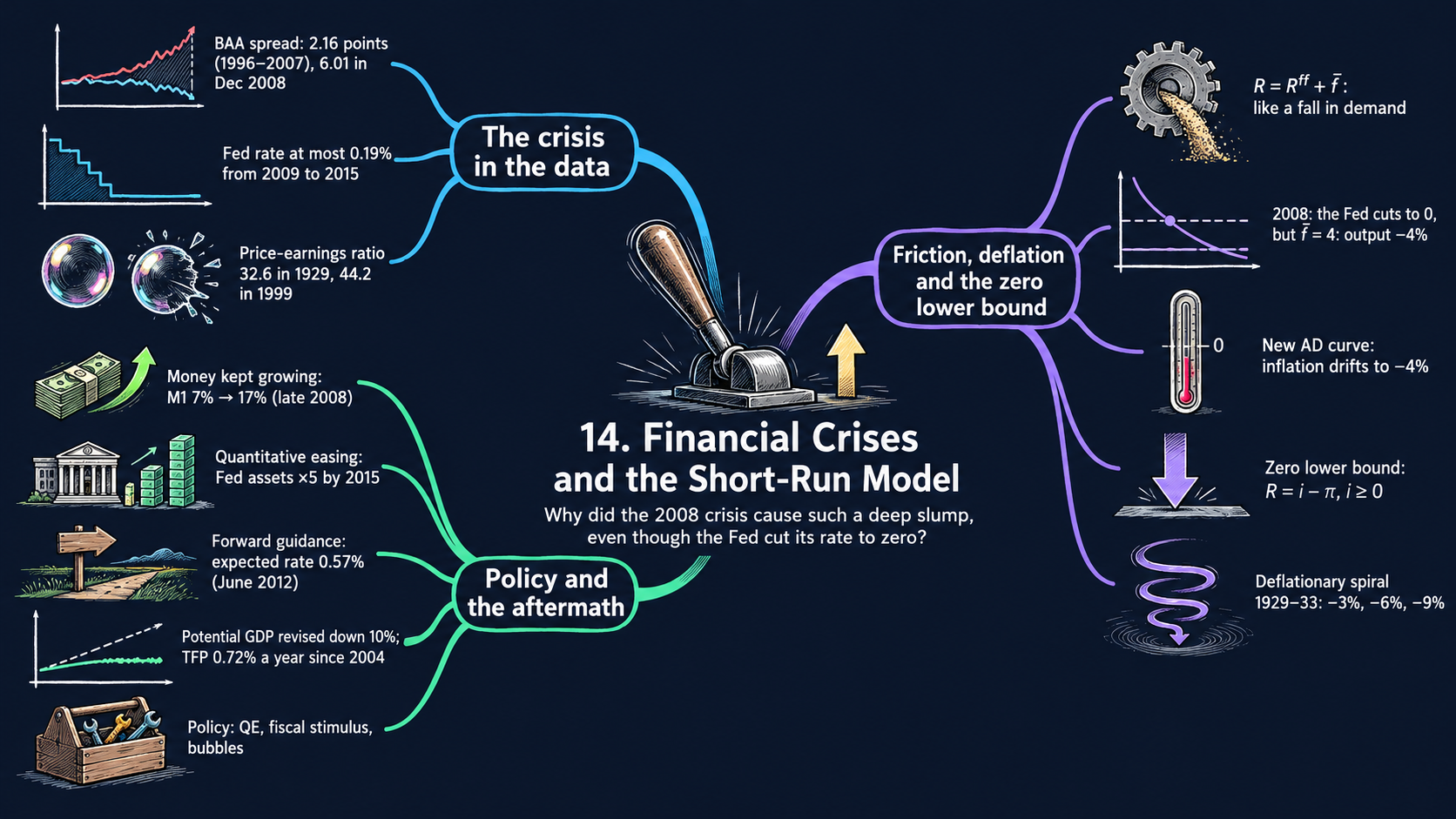
Learning goals

Chapters 11 to 13 assumed that the central bank sets the interest rate at which firms and households borrow. In a financial crisis that link breaks. This chapter adds a risk premium to the short-run model and uses it, together with U.S. data, to study the financial crisis of 2008–2009, the dangers of deflation and the policy response. By the end of it you will be able to:

add the financial friction $\bar{f}$ to the IS/MP model, derive the new AD curve step by step, and show why the friction acts like a negative demand shock;
solve the AS/AD model period by period for output and inflation, derive the long run and the speed of adjustment, and read the comparative statics of a higher risk premium;
derive the best output the Fed can reach at the zero lower bound, and show with the Fisher equation why a deflationary spiral can turn a recession into a depression;
use balance-sheet algebra (leverage, capital requirements), present values and the term structure to explain the policy responses: bank rescues, quantitative easing, forward guidance and fiscal stimulus;
read the data on the crisis and its aftermath (interest-rate spreads, the Taylor rule, potential GDP, money growth, asset-price bubbles, the Fed’s balance sheet, forward guidance and productivity), and compare the U.S. experience with dozens of other economies;
in Python: build a model step by step from small functions, compute peaks, troughs and growth rates, stack a chart with px.area, rebuild a table from monthly data, blank out data that cross a definition break, and pick countries from a list (SelectMultiple) with a color that stays fixed for each country.

Model overview

Islandia has had a good run, until a housing boom on the island turns to bust and fear spreads through its banks. Lenders now ask Harbor Boatworks and the islanders for a much higher rate than before, even though the Bank of Islandia is cutting its own rate as fast as it can. Prices start to fall, and the central bank soon has no room left to cut. Can a scare in the banks drag a whole island into a deep slump, and what can policy do about it? This section adds the missing link, a risk premium, to the short-run model of Chapters 11 to 13 and follows Islandia through the crisis.

The big idea

The question. Why can a financial crisis cause a deep recession even when the central bank cuts its interest rate all the way to zero?

The answer in one sentence. Firms and households borrow at the central bank’s rate plus a premium, so a jump in that financial friction hits spending exactly like a fall in demand, and at the zero lower bound falling prices push the real rate up and can start a deflationary spiral.

What goes in and what comes out. We choose the demand shock, the risk premium, the inflation target, how hard the central bank reacts, the slope of the Phillips curve and, for the policy block, the balance-sheet and asset-price numbers. The model gives back output, inflation and interest rates year by year, the best output the central bank can reach at the zero bound, and how much a bank or a share loses in a crash.

Road map.

The IS/MP model with a financial friction: the assumptions, solving the model step by step, and what the model predicts.
The new AD curve: the friction in the AS/AD model, solved period by period, with its long run and comparative statics.
Deflation and the zero lower bound: the Fisher equation, the floor on the real rate and the deflationary spiral.
Balance sheets, leverage and the policy responses: the definitions, the algebra of leverage, asset prices, quantitative easing, forward guidance and fiscal stimulus, and a table of the policies.
Model in code: the key results as Python functions, checked with numbers, followed by the drawing tools for the diagrams and the tools for the data figures (recession shading and a peak-to-trough calculator).

Notation. A bar over a letter marks a parameter, a number set outside the model; letters without a bar are endogenous variables that the model solves for. Short-run output $\tilde{Y}_t$ is the percentage gap between actual and potential output, and all interest and inflation rates are in percent per year. In the code we write a, f, m, B_BAR, NU, and so on.

Symbol	Meaning	Type
$\tilde{Y}_t$	short-run output: the percent gap between actual and potential output	endogenous
$R_t$	the real rate that firms and households pay on their loans	endogenous
$R^{ff}_t$	the real fed funds rate: the central bank’s own policy rate	endogenous
$\pi_t$, $\pi^e_t$	inflation, and the inflation people expect	endogenous
$i_t$, $i^{ff}_t$, $i^L_t$	nominal rates: the borrowing rate, the fed funds rate, an $n$-year rate	endogenous
$\bar{a}$, $\bar{b}$, $\bar{r}$	the demand shock, the interest sensitivity of demand, the marginal product of capital	parameters
$\bar{f}$	the risk premium (the financial friction)	parameter
$\bar{\pi}$, $\bar{m}$, $\bar{x}$	the inflation target, the response to inflation, the response to output	parameters
$\bar{\nu}$	the slope of the Phillips curve	parameter
$\bar{i}$	a nominal rate that is stuck (at the bound, or by choice)	parameter
$\pi_C$, $\tilde{Y}^{\max}_t$	long-run inflation; the best output reachable at the zero lower bound	endogenous
$\lambda$, $\kappa$	leverage and the capital ratio of a balance sheet	endogenous
$P$, $E$, $g$	an asset’s price, next year’s profits, and their growth rate	notation
$R^{ff,*}$, $x_t$	the rate that restores potential output; inflation’s distance from $\pi_C$	notation

The IS/MP model with a financial friction

Assumptions

Islandia in numbers. The textbook draws its diagrams without numbers, apart from a few examples. Here the algebra, the checks and every diagram of the notebook share one illustrative baseline:

the IS curve: a marginal product of capital $\bar{r} = 2$ percent and $\bar{b} = 1$, so each point of interest rate above $\bar{r}$ costs 1 percent of output;
the policy rule and the Phillips curve: an inflation target $\bar{\pi} = 2$ percent, $\bar{m} = 1$ and $\bar{\nu} = 0.5$;
the 2008 scenario: a housing bust lowers demand by $\bar{a}' = -2$, and the panic adds a risk premium $\bar{f} = 4$ points;
the 1929 scenario: the central bank raises its rate by 3 points, and a stock market crash lowers demand by $\bar{a}' = -3$.

The two scenarios are named after the U.S. episodes that the figures study. With these values the model gives the textbook’s example numbers: $-2$ and $-4$ percent in Fig. 2, and $-3$, $-6$ and $-9$ percent in Figs. 12 and 13.

1. The IS curve (Chapter 11). Harbor Boatworks invests less, and islanders spend less, when the real rate $R_t$ they pay climbs above the marginal product of capital $\bar{r}$. Short-run output follows:

\[\tilde{Y}_t = \bar{a} - \bar{b}\,(R_t - \bar{r}).\]

The demand shock $\bar{a}$ gathers every reason to spend more or less at a given interest rate: confidence, household wealth, government purchases, exports. The parameter $\bar{b} > 0$ says how strongly investment responds to the rate.

2. The central bank sets the fed funds rate. The Bank of Islandia controls the (real) fed funds rate $R^{ff}_t$, the overnight rate at which Islandia’s banks lend to one another. (We keep the U.S. name, since the data come from there.) Chapters 11 to 13 treated this as the rate that firms pay. From now on it is not.

3. The financial friction. Islandia’s banks add a premium $\bar{f} \geq 0$ on top of the fed funds rate when they lend to firms and households. It pays them for the chance that a loan goes bad:

\[R_t = R^{ff}_t + \bar{f}. \tag{1}\]

In quiet years $\bar{f}$ is near zero, and the central bank in effect sets the borrowing rate itself. In a panic $\bar{f}$ shoots up. Fig. 1 measures it in the data as the gap between the yields on corporate and government bonds.

Solving the model

Step 1: the IS curve in terms of the Fed’s rate. Replace $R_t$ in the IS curve by equation (1), then pull $\bar{f}$ out of the bracket:

\[\tilde{Y}_t = \bar{a} - \bar{b}\,(R^{ff}_t + \bar{f} - \bar{r}) = \bar{a} - \bar{b}\bar{f} - \bar{b}\,(R^{ff}_t - \bar{r}).\]

The first two terms do not depend on the central bank, so they form one combined demand shock, $\bar{a} - \bar{b}\bar{f}$.

In words

Harbor Boatworks does not ask why its loan got dearer. Whether the central bank raised its rate or the banks raised their premium, the boatyard pays more and builds fewer boats. So, seen from the rate the Bank of Islandia controls, a bigger premium looks just like a drop in demand.

Step 2: the rate that restores potential output. Suppose the central bank wants $\tilde{Y}_t = 0$. Set the left side to zero, move $\bar{b}(R^{ff}_t - \bar{r})$ across and divide by $\bar{b}$ (Appendix C.9):

\[0 = \bar{a} - \bar{b}\bar{f} - \bar{b}\,(R^{ff}_t - \bar{r}) \quad\Longrightarrow\quad R^{ff}_t - \bar{r} = \frac{\bar{a}}{\bar{b}} - \bar{f}.\]

Key result: the IS curve with a financial friction

\[\tilde{Y}_t = \underbrace{\bar{a} - \bar{b}\bar{f}}_{\text{demand shock}} - \bar{b}\,(R^{ff}_t - \bar{r}) \tag{2}\]

\[R^{ff,*} = \bar{r} + \frac{\bar{a}}{\bar{b}} - \bar{f} \tag{3}\]

Equation (2) is the IS curve drawn against the rate the central bank sets. Equation (3) says that the bank must offset the demand shock (the term $\bar{a}/\bar{b}$) and cut one extra point for each point of premium.

Islandia in numbers. In the 2008 scenario, $\bar{a}' = -2$ and $\bar{f} = 4$, so (3) asks for $R^{ff,*} = 2 - 2 - 4 = -4$ percent.

Step 3: the 2008 example in numbers. With $\bar{a}' = -2$ and $\bar{b} = 1$, the crisis comes in three stages:

the housing bust, and the central bank does nothing ($R^{ff} = \bar{r} = 2$, $\bar{f} = 0$): $\tilde{Y} = -2 - 0 = -2$ percent (point $B$ of Fig. 2);
the bank cuts to the rate (3) with $\bar{f} = 0$: $R^{ff} = 2 + (-2)/1 = 0$ percent and $\tilde{Y} = 0$ (point $C$);
the panic adds $\bar{f} = 4$, but the bank stays at 0: Harbor Boatworks pays $R = 0 + 4 = 4$ percent, and $\tilde{Y} = -2 - 1\times(4 - 2) = -4$ percent (point $D$).

Getting output back to potential would take a fed funds rate of $-4$ percent. The third block explains why the central bank cannot go that low.

The rate that matters for spending is the central bank’s rate plus the risk premium, so a panic acts like a demand shock.

What the model predicts

Comparative statics. Equation (2) is a straight line, so each effect is a fixed number: the derivative of $\tilde{Y}_t$ with respect to that parameter (Appendix C.7).

A one-point rise in …	changes $\tilde{Y}_t$ by	What moves in the IS/MP diagram	What the central bank must do, from (3)
the risk premium $\bar{f}$	$-\bar{b} = -1$ point	the MP line (the rate firms pay) shifts up by 1	cut $R^{ff}$ by 1 point
the fed funds rate $R^{ff}$	$-\bar{b} = -1$ point	the MP line shifts up by 1	(this is the bank’s tool)
the demand shock $\bar{a}$	$+1$ point	the IS curve shifts right by 1	raise $R^{ff}$ by $1/\bar{b} = 1$ point

A friction is a demand shock. At a fixed policy rate, one more point of $\bar{f}$ costs $\bar{b}$ points of output, the same as a fall of $\bar{a}$ by $\bar{b}$.
The central bank can undo it, point for point, as long as it is free to cut $R^{ff}$ far enough. With $\bar{f} = 2$ in our example, the premium cancels the bank’s cut of 2 points, and $D$ falls on top of $B$.
Two shocks add up. Against the bank’s starting rate, the bust and the premium together cost $\bar{a}' - \bar{b}\bar{f}$. Once the cut has offset the bust, what remains is $-\bar{b}\bar{f} = -4$ percent.

Each point of premium needs one extra point of rate cuts, which is easy in normal times and impossible near zero.

Check your understanding

1. A milder panic hits Islandia: the housing bust is still $\bar{a}' = -2$, but the premium is only $\bar{f} = 2$. The central bank has cut its rate to 0 percent. What is short-run output, and what fed funds rate would close the gap?

Answer

By the IS curve with equation (1), firms pay $R = 0 + 2 = 2$ percent, so $\tilde{Y} = -2 - 1\times(2 - 2) = -2$ percent: the premium has undone the whole cut. Equation (3) asks for $R^{ff,*} = 2 - 2 - 2 = -2$ percent.

2. On the IS/MP diagram, does a higher premium shift the IS curve or the MP line?

Answer

The MP line, if we plot the rate that firms pay: equation (1) lifts it by $\bar{f}$ at any fed funds rate. Plotted against the fed funds rate instead, equation (2) shows the same event as a shift of the IS curve to the left by $\bar{b}\bar{f}$. Both views give the same output.

The new AD curve: a financial friction in the AS/AD model

Assumptions

Keep the IS curve and equation (1). Add the other two pieces of the AS/AD model of Chapter 13:

4. A monetary policy rule. The Bank of Islandia moves its rate with the gap between inflation and its target,

\[R^{ff}_t - \bar{r} = \bar{m}\,(\pi_t - \bar{\pi}), \qquad \bar{m} > 0.\]

5. The AS curve. The Phillips curve with adaptive expectations ($\pi^e_t = \pi_{t-1}$): inflation climbs above last year’s rate when output is above potential,

\[\pi_t = \pi_{t-1} + \bar{\nu}\,\tilde{Y}_t.\]

Each year the model solves for four unknowns, $\tilde{Y}_t$, $\pi_t$, $R^{ff}_t$ and $R_t$. Last year’s inflation $\pi_{t-1}$ is already known.

Solving the model

Step 1: the borrowing rate under the rule. Put the rule into equation (1). Take $\bar{r}$ away from both sides of (1) first:

\[R_t - \bar{r} = (R^{ff}_t - \bar{r}) + \bar{f} = \bar{f} + \bar{m}\,(\pi_t - \bar{\pi}).\]

Whatever rate the rule sets, Islandia’s banks add the premium on top.

Step 2: the new AD curve. Put this into the IS curve and group the terms that do not depend on inflation:

\[\tilde{Y}_t = \bar{a} - \bar{b}\left[\bar{f} + \bar{m}\,(\pi_t - \bar{\pi})\right].\]

Key result: the new AD curve

\[\tilde{Y}_t = \underbrace{\bar{a} - \bar{b}\bar{f}}_{\text{AD shock}} - \bar{b}\bar{m}\,(\pi_t - \bar{\pi}) \tag{4}\]

It is the AD curve of Chapter 13 with $\bar{a}$ replaced by $\bar{a} - \bar{b}\bar{f}$. It slopes down: higher inflation makes the central bank raise its rate, and output falls.

To draw it with inflation on the vertical axis, solve (4) for $\pi_t$:

\[\pi_t = \bar{\pi} + \frac{\bar{a} - \bar{b}\bar{f} - \tilde{Y}_t}{\bar{b}\bar{m}}.\]

Step 3: this period’s output and inflation. Islandia sits where AD and AS cross. Replace $\pi_t$ in (4) by the AS curve $\pi_{t-1} + \bar{\nu}\tilde{Y}_t$:

\[\tilde{Y}_t = \bar{a} - \bar{b}\bar{f} - \bar{b}\bar{m}\,(\pi_{t-1} - \bar{\pi}) - \bar{b}\bar{m}\bar{\nu}\,\tilde{Y}_t.\]

Gather the $\tilde{Y}_t$ terms on the left, $(1 + \bar{b}\bar{m}\bar{\nu})\,\tilde{Y}_t = \bar{a} - \bar{b}\bar{f} - \bar{b}\bar{m}(\pi_{t-1} - \bar{\pi})$, and divide:

Key result: output and inflation each year

\[\tilde{Y}_t = \frac{\bar{a} - \bar{b}\bar{f} - \bar{b}\bar{m}\,(\pi_{t-1} - \bar{\pi})}{1 + \bar{b}\bar{m}\bar{\nu}}, \qquad \pi_t = \pi_{t-1} + \bar{\nu}\,\tilde{Y}_t \tag{5}\]

Given last year’s inflation, the first formula gives this year’s output, and the AS curve then gives this year’s inflation.

Islandia in numbers. With $\bar{b} = \bar{m} = 1$ and $\bar{\nu} = 0.5$ the denominator is $1.5$. In the first year of the 2008 scenario $\pi_{t-1} = \bar{\pi} = 2$, so $\tilde{Y}_1 = (-2 - 4 - 0)/1.5 = -4$ percent and $\pi_1 = 2 + 0.5\times(-4) = 0$ percent: point $B$ of Fig. 3.

In words: the rule as a shock absorber

The AD shock is $-6$, yet output falls by only 4 percent in the first year. The reason is the rule. As the slump pulls inflation down, the Bank of Islandia cuts its rate, and that cut softens the blow to Harbor Boatworks. Without any response, the whole shock of 6 points would land on output.

Step 4: the long run. If the shocks persist, Islandia settles where inflation stops changing. By the AS curve, $\pi_t = \pi_{t-1}$ only when $\tilde{Y}_t = 0$. Set $\tilde{Y} = 0$ in (4) and solve for inflation:

\[0 = \bar{a} - \bar{b}\bar{f} - \bar{b}\bar{m}\,(\pi_C - \bar{\pi}) \quad\Longrightarrow\quad \pi_C - \bar{\pi} = \frac{\bar{a} - \bar{b}\bar{f}}{\bar{b}\bar{m}}.\]

Step 5: how fast the economy gets there. Measure inflation by its distance from the long run, $x_t \equiv \pi_t - \pi_C$. Step 4 says $\bar{a} - \bar{b}\bar{f} = \bar{b}\bar{m}(\pi_C - \bar{\pi})$. Use this in the numerator of (5):

\[\bar{b}\bar{m}(\pi_C - \bar{\pi}) - \bar{b}\bar{m}(\pi_{t-1} - \bar{\pi}) = -\bar{b}\bar{m}\,(\pi_{t-1} - \pi_C) = -\bar{b}\bar{m}\,x_{t-1}, \qquad\text{so}\qquad \tilde{Y}_t = \frac{-\bar{b}\bar{m}\,x_{t-1}}{1 + \bar{b}\bar{m}\bar{\nu}}.\]

Next, subtract $\pi_C$ from both sides of the AS curve and insert this expression for $\tilde{Y}_t$:

\[x_t = x_{t-1} + \bar{\nu}\tilde{Y}_t = x_{t-1}\left(1 - \frac{\bar{b}\bar{m}\bar{\nu}}{1 + \bar{b}\bar{m}\bar{\nu}}\right) = \frac{x_{t-1}}{1 + \bar{b}\bar{m}\bar{\nu}}.\]

Repeat this step $t$ times (Appendix C.10) to reach the result below.

Key result: the long run and the speed of adjustment

\[\pi_C = \bar{\pi} + \frac{\bar{a} - \bar{b}\bar{f}}{\bar{b}\bar{m}} \tag{6}\]

\[\pi_t - \pi_C = \left(\frac{1}{1 + \bar{b}\bar{m}\bar{\nu}}\right)^{t}(\pi_0 - \pi_C) \tag{7}\]

Output goes back to potential, but inflation ends at $\pi_C$, and each year the remaining gap shrinks by the same factor.

Islandia in numbers. $\pi_C = 2 + (-6)/1 = -4$ percent: output recovers at point $C$, but with deflation. With a factor of $1/1.5$, one third of the gap closes each year. From $\pi_0 - \pi_C = 6$, inflation goes to $\pi_1 = 0$ and then $\pi_2 = -4 + 6\times\tfrac{4}{9} \approx -1.3$ percent, on its way to $-4$.

By the formula for $\tilde{Y}_t$ in Step 5, output runs $-4$, then $-2.7$, then $-1.8$ percent. Inflation keeps falling until the rule has cut the borrowing rate far enough to offset both shocks.

Under a policy rule the slump fades year by year, but inflation ends lower, possibly below zero.

Check your understanding

1. Suppose the Bank of Islandia reacts twice as hard, $\bar{m} = 2$, in the 2008 scenario. What is output in the first year, and what share of the remaining inflation gap closes each year?

Answer

Now $1 + \bar{b}\bar{m}\bar{\nu} = 1 + 1\times2\times0.5 = 2$. By equation (5), $\tilde{Y}_1 = -6/2 = -3$ percent instead of $-4$. By equation (7) the gap is multiplied by $1/2$ each year, so half of it closes every year, faster than the one third of the baseline.

What the model predicts

Comparative statics. Each effect follows from equations (5) and (6) by differentiating with respect to one parameter. The numbers use our baseline, $1 + \bar{b}\bar{m}\bar{\nu} = 1.5$.

A one-point rise in …	AD curve	output in the first year	inflation in the first year	long-run inflation $\pi_C$	long-run output
the demand shock $\bar{a}$	shifts right by 1	$+\frac{1}{1.5} = +0.67$	$+\frac{\bar{\nu}}{1.5} = +0.33$	$+\frac{1}{\bar{b}\bar{m}} = +1$	0
the risk premium $\bar{f}$	shifts left by $\bar{b} = 1$	$-\frac{\bar{b}}{1.5} = -0.67$	$-0.33$	$-\frac{1}{\bar{m}} = -1$	0

The friction is an AD shock. A higher $\bar{f}$ moves the AD curve toward lower output at every inflation rate, just as a lower $\bar{a}$ would. The AS curve stays put at first. That is Fig. 3.
The recession passes; the lower inflation stays. Output returns to potential, but inflation settles $1/\bar{m}$ lower for each point of premium. Starting from just 2 percent, a big enough shock ends in deflation: $\pi_C < 0$ whenever $\bar{a} - \bar{b}\bar{f} < -\bar{b}\bar{m}\bar{\pi}$, here whenever the AD shock is worse than $-2$.
A tougher rule helps. A larger $\bar{m}$ flattens AD. The first-year recession $(\bar{a} - \bar{b}\bar{f})/(1 + \bar{b}\bar{m}\bar{\nu})$ gets smaller, $\pi_C$ falls by less, and by (7) the economy converges faster.
The hidden assumption. The rule must always be able to deliver the real rate it calls for. The next block shows how deflation and the zero lower bound break this, which is why the textbook turns to the IS/MP diagram for such times (Figs. 12 and 13).

A risk premium shifts AD left: a temporary recession, but a permanent fall in inflation.

Check your understanding

1. A milder panic: $\bar{a}' = -2$ and $\bar{f} = 2$, starting from $\pi_0 = 2$. What are output and inflation in the first year, and where does inflation end up?

Answer

The AD shock is $-2 - 2 = -4$. By equation (5), $\tilde{Y}_1 = -4/1.5 \approx -2.7$ percent and $\pi_1 = 2 + 0.5\times(-2.67) \approx 0.7$ percent. By equation (6), $\pi_C = 2 + (-4)/1 = -2$ percent: even this milder panic ends in deflation.

2. Does the risk premium lower Islandia’s output in the long run?

Answer

No. By the AS curve, inflation keeps falling as long as output is below potential, and every fall makes the rule cut the rate. The economy only comes to rest at $\tilde{Y} = 0$. The premium shows up in the long run as lower inflation, $1/\bar{m}$ per point by equation (6), not as lower output.

Deflation and the zero lower bound

Assumptions

6. The Fisher equation (Chapter 12). The nominal interest rate $i_t$ is the real rate plus inflation, $i_t = R_t + \pi_t$. Take $\pi_t$ from both sides to get the real rate, the one in the IS curve:

\[R_t = i_t - \pi_t. \tag{8}\]

(The textbook prints this rearranged equation with a plus sign in place of the minus. That is a typo: the surrounding text uses the minus.) The same link holds for the central bank’s rate: the nominal fed funds rate is $i^{ff}_t = R^{ff}_t + \pi_t$.

7. The zero lower bound. A nominal rate cannot go (much) below zero, $i^{ff}_t \geq 0$. Islanders can always keep cash under the mattress, and cash earns exactly zero, so nobody would lend at less.

Solving the model

Step 1: the nominal rate a rule asks for. Add $\pi_t$ to both sides of the policy rule, and let the rate react to output as well (the Taylor rule of Chapter 13, with weight $\bar{x}$ on output):

\[i^{ff}_t = R^{ff}_t + \pi_t = \bar{r} + \pi_t + \bar{m}\,(\pi_t - \bar{\pi}) + \bar{x}\,\tilde{Y}_t. \tag{9}\]

Taylor’s original values, $\bar{r} = \bar{\pi} = 2$ and $\bar{m} = \bar{x} = 0.5$, give $i^{ff}_t = 2 + \pi_t + 0.5\pi_t - 1 + 0.5\tilde{Y}_t = 1 + 1.5\,\pi_t + 0.5\,\tilde{Y}_t$, the rule drawn in Fig. 4. In our AS/AD baseline ($\bar{m} = 1$, $\bar{x} = 0$) it reads $i^{ff}_t = 2 + \pi_t + (\pi_t - 2) = 2\pi_t$. So the rule wants a negative nominal rate as soon as inflation turns negative, which on the path of equation (7) happens from period 2 on. Fig. 3 silently assumes a cut that the Bank of Islandia could not make.

Step 2: the floor on the real rate. Put $i^{ff}_t \geq 0$ into $R^{ff}_t = i^{ff}_t - \pi_t$: the real fed funds rate can go no lower than $-\pi_t$. By equation (1), the lowest rate Harbor Boatworks can pay is then $\bar{f} - \pi_t$.

Step 3: the best output the central bank can reach. Put this lowest borrowing rate into the IS curve:

\[\tilde{Y}^{\max}_t = \bar{a} - \bar{b}\,(\bar{f} - \pi_t - \bar{r}).\]

Multiply out the bracket and collect the terms in $\bar{r}$ and $\pi_t$:

Key result: the best output at the zero lower bound

\[\tilde{Y}^{\max}_t = \bar{a} - \bar{b}\bar{f} + \bar{b}\,(\bar{r} + \pi_t) \tag{10}\]

The bound binds when the rate the bank needs, (3), lies below the floor, $R^{ff,*} < -\pi_t$, which is the same as $\tilde{Y}^{\max}_t < 0$.

Islandia in numbers (2008 scenario, $\bar{a}' = -2$, $\bar{f} = 4$). With inflation at 2 percent, $\tilde{Y}^{\max} = -2 - 4 + 1\times(2 + 2) = -2$ percent, so even a zero nominal rate only gets output back to $B$. With zero inflation the best is $-4$ percent, and with 2 percent deflation it is $-6$ percent.

In words

At the bound, inflation becomes the Bank of Islandia’s last lever on the real rate. While prices rise, a zero nominal rate still means a negative real rate, which helps Harbor Boatworks. Once prices fall, the same zero nominal rate means a positive real rate, and the best the bank can do gets worse with every point of deflation.

Step 4: the deflationary spiral. Now let the nominal rate be stuck at some $\bar{i}$, either at the bound or because the central bank will not move it (as the Fed did in the early 1930s). Borrowers judge the real rate by the inflation they expect, which under adaptive expectations is last year’s: $R_t = \bar{i} - \pi_{t-1} + \bar{f}$. The IS curve turns into

\[\tilde{Y}_t = \bar{a} - \bar{b}\,(\bar{i} + \bar{f} - \bar{r}) + \bar{b}\,\pi_{t-1}.\]

Write the same equation for the year before and subtract it. All the terms with a bar drop out:

\[\tilde{Y}_t - \tilde{Y}_{t-1} = \bar{b}\,(\pi_{t-1} - \pi_{t-2}) = \bar{b}\bar{\nu}\,\tilde{Y}_{t-1},\]

where the last step uses the AS curve one year back, $\pi_{t-1} - \pi_{t-2} = \bar{\nu}\tilde{Y}_{t-1}$. Add $\tilde{Y}_{t-1}$ to both sides:

Key result: the deflationary spiral

\[\tilde{Y}_t = (1 + \bar{b}\bar{\nu})\,\tilde{Y}_{t-1} \tag{11}\]

With the nominal rate frozen, each year’s output gap is a fixed multiple, larger than one, of last year’s.

Islandia in numbers. $1 + \bar{b}\bar{\nu} = 1.5$, so a gap of $-6$ percent becomes $-9$, then $-13.5$ percent: the slump deepens by 50 percent each year.

This is the step from $C$ to $D$ in Figs. 12 and 13 (the 1929 scenario). The crash leaves output at $-6$ percent with inflation at zero. The slump then drags inflation to $0 + 0.5\times(-6) = -3$ percent, the real rate rises by 3 points, and output sinks to $-9$ percent.

At the zero lower bound falling prices raise the real rate, and a slump can feed on itself.

What the model predicts

Deflation raises the real rate. By (8), with $i_t$ fixed, each point less of inflation adds a point to the real rate. In normal times the central bank just cuts $i_t$; at the zero lower bound it has no room.
Comparative statics at the bound, from equation (10): $\partial\tilde{Y}^{\max}/\partial\pi = +\bar{b}$ (each point of deflation costs $\bar{b} = 1$ point of reachable output), $\partial\tilde{Y}^{\max}/\partial\bar{f} = -\bar{b}$, and $\partial\tilde{Y}^{\max}/\partial\bar{a} = +1$. In the IS/MP diagram, deflation and a higher premium both push the lowest possible MP line up.
Stable versus unstable. Put equations (7) and (11) side by side. Under a rule with $\bar{m} > 0$, falling inflation lowers the real rate, and the gap shrinks by the factor $1/(1 + \bar{b}\bar{m}\bar{\nu}) < 1$ each year. With the nominal rate frozen, falling inflation raises the real rate, and the gap grows by the factor $1 + \bar{b}\bar{\nu} > 1$. The only resting point is $\tilde{Y} = 0$, and the economy drifts away from it: a deflationary spiral. In the terms of equation (4), a frozen nominal rate works like a rule with a negative $\bar{m}$.
Ways out. Anything that raises $\tilde{Y}^{\max}$ in (10) helps:
- a higher $\bar{a}$ (fiscal stimulus by the Islandia Treasury);
- a lower $\bar{f}$ (rescuing the banks);
- higher expected inflation (anchored expectations, money growth);
- lower long-term rates through asset purchases and forward guidance.
The next block puts numbers on these. Secular stagnation is the case in which $R^{ff,*}$ in (3) stays below the floor for years.

Check your understanding

1. In the 2008 scenario ($\bar{a}' = -2$, $\bar{f} = 4$), Islandia’s inflation has slipped to 1 percent and the nominal rate is at zero. What is the best output the central bank can reach?

Answer

By equation (10), $\tilde{Y}^{\max} = -2 - 4 + 1\times(2 + 1) = -3$ percent. The bound binds: even at a zero rate, output stays 3 percent below potential.

2. Islandia’s nominal rate is frozen, and output is 4 percent below potential this year. What does the model predict for next year, and why does the slump get worse?

Answer

By equation (11), next year’s gap is $1.5\times(-4) = -6$ percent. The slump lowers inflation by $\bar{\nu}\times4 = 2$ points. With the nominal rate stuck, the Fisher equation (8) turns that into a real rate 2 points higher, which costs $\bar{b}\times2 = 2$ more points of output.

Balance sheets, leverage and the policy responses

Definitions

Balance sheet. For one of Islandia’s banks, a household or the central bank, what it owns equals what it owes plus what is left over for its owners:

\[\text{Assets} = \text{Liabilities} + \text{Net worth}.\]

Leverage (Chapter 10) is the ratio of liabilities to net worth, $\lambda \equiv \text{Liabilities}/\text{Net worth}$. A capital requirement sets a minimum for the capital ratio $\kappa \equiv \text{Net worth}/\text{Assets}$.

Present value. An asset that pays profits $E$ next year, growing at the rate $g$ every year after that, is worth the sum of those profits discounted at the interest rate $R > g$ (Appendix C.12).

The term structure (Chapter 12). An $n$-year interest rate is roughly the average of the short rates expected over the next $n$ years.

Solving the model

Step 1: leverage and the capital ratio. Divide the balance sheet by net worth: $\text{Assets}/\text{Net worth} = \lambda + 1$. The capital ratio $\kappa$ is the inverse of that ratio, so

\[\kappa = \frac{1}{1 + \lambda} \qquad\Longleftrightarrow\qquad \lambda = \frac{1 - \kappa}{\kappa}.\]

A capital requirement is therefore a cap on leverage. A 7 percent requirement permits $\lambda = 0.93/0.07 \approx 13.3$; a 20 percent requirement permits only $\lambda = 4$.

Step 2: why leverage magnifies losses. A bank’s debts are fixed in money terms. If its assets lose the share $x$ of their value, the entire loss, $x\cdot\text{Assets}$, falls on net worth. As a share of net worth:

\[\frac{\Delta\,\text{Net worth}}{\text{Net worth}} = -\,x\,\frac{\text{Assets}}{\text{Net worth}}.\]

Since $\text{Assets}/\text{Net worth} = 1 + \lambda = 1/\kappa$:

Key result: leverage magnifies losses

\[\frac{\Delta\,\text{Net worth}}{\text{Net worth}} = -(1 + \lambda)\,x = -\frac{x}{\kappa} \tag{12}\]

Islandia in numbers. A bank with a 7 percent capital ratio loses $3/0.07 \approx 43$ percent of its net worth when its assets lose 3 percent. It is insolvent (net worth below zero) once they lose more than $\kappa = 7$ percent. A 20 percent ratio absorbs a 20 percent fall.

In words

Think of an Islandia bank’s capital as a cushion between its assets and its depositors. Leverage measures how thin that cushion is. A small fall in house prices goes straight through a thin cushion, which is why lenders panic and raise $\bar{f}$. When the Islandia Treasury injects capital into a bank (as TARP did in the United States), it thickens the cushion and lowers $\lambda$.

Step 3: asset prices. The present value of the growing stream of profits is a geometric series with ratio $q = (1+g)/(1+R) < 1$:

\[P = \frac{E}{1+R} + \frac{E(1+g)}{(1+R)^2} + \frac{E(1+g)^2}{(1+R)^3} + \dots = \frac{E}{1+R}\cdot\frac{1}{1 - q} = \frac{E}{1+R}\cdot\frac{1+R}{R - g}.\]

Divide both sides by $E$:

Key result: the price-earnings ratio

\[\frac{P}{E} = \frac{1}{R - g} \tag{13}\]

Islandia in numbers. If shares in Harbor Boatworks are priced with $R = 7$ percent and $g = 2$ percent, $P/E = 1/0.05 = 20$. One more point on the discount rate, say from a higher risk premium, gives $1/0.06 \approx 16.7$: share prices drop by about 17 percent.

Take logs (Appendix C.4): $\ln P = \ln E - \ln(R - g)$, so $d\ln P/dR = -1/(R - g) = -20$. A rise in $R$ of 0.01 (one point) lowers $\ln P$ by about 0.2. That is the slope at the baseline; over a whole point the exact fall is the 17 percent above, because the slope flattens as $R - g$ widens. A ratio far above anything plausible values of $R - g$ can justify signals a bubble (Figs. 7 and 8). When such prices collapse, islanders’ wealth shrinks and $\bar{a}$ falls.

Step 4: the Fed’s balance sheet. For the central bank the identity is

\[\text{Treasuries} + \text{MBS} + \text{other assets} = \text{Currency} + \text{Reserves} + \text{other liabilities}.\]

Quantitative easing buys assets other than short-term government bonds, such as mortgage-backed securities (MBS) or long-term Treasuries. The central bank pays by crediting reserves to the sellers’ banks, so both sides grow by the same amount and no new currency is printed. Table 14.1 (in the Key numbers of Fig. 9) checks this identity in the U.S. data.

Step 5: forward guidance. Write the $n$-year rate as the average of the expected short rates,

\[i^{L}_t \approx \frac{i_t + i^e_{t+1} + \dots + i^e_{t+n-1}}{n}. \tag{14}\]

Even with today’s rate $i_t$ stuck at zero, the central bank can push the long rate down by promising to keep future rates low. Take a 4-year bond. If markets expect short rates of 0, 1, 2 and 3 percent, the long rate is $6/4 = 1.5$ percent. A believable promise of zero for three years (0, 0, 0, 2) brings it down to $2/4 = 0.5$ percent. Fig. 10 shows such a shift in market expectations.

Step 6: fiscal stimulus at the bound. Government purchases are part of $\bar{a}$. At the zero lower bound the interest rate does not rise when $\bar{a}$ goes up, so by equation (10) a stimulus lifts reachable output one for one: closing the gap takes $\Delta\bar{a} = -\tilde{Y}^{\max}$. In the 2008 scenario that is 2 percent of potential output with inflation at 2 percent, but 6 percent once 2 percent deflation has set in. Delay makes the job bigger.

Thin capital cushions turn small price falls into bank failures, and a panic about them is what lifts the risk premium.

What the model predicts

Policy	Which term it moves	Effect
cut the fed funds rate	$R^{ff}$ in (2)	works until the floor $-\pi$ of (10)
rescue banks (TARP), higher capital ratios	$\bar{f}$ in (1), $\lambda$ in (12)	lower premium; smaller losses in the next crisis
quantitative easing	long-term and mortgage rates, (13) and (14)	lower borrowing rates beyond the fed funds rate
forward guidance	expected future rates in (14)	lower long rates at a zero short rate
fiscal stimulus	$\bar{a}$ in (2) and (10)	raises output one for one at the bound
anchored inflation expectations	$\pi$ in (10), the spiral (11)	keeps the real rate from rising

Leverage turns small price falls into crises. By (12), a fall in asset prices of a few percent can wipe out a highly leveraged bank. The fear of such losses is what raises $\bar{f}$.
Higher capital requirements shrink $1 + \lambda$ in (12). They are the most direct way to make the next crisis smaller.
Asset prices react strongly to the discount rate when $R - g$ is small, by (13). Booms and busts in share and home prices move islanders’ wealth, and so $\bar{a}$.

When the policy rate is stuck at zero, policy works on the other terms: the premium, long rates, expectations and spending.

Check your understanding

1. An Islandia bank holds a capital ratio of 10 percent. What is its leverage, and how much of its net worth does it lose if its assets fall by 4 percent?

Answer

By Step 1, $\lambda = (1 - 0.1)/0.1 = 9$. By equation (12), net worth falls by $4/0.1 = 40$ percent. A fall of more than 10 percent in its assets would leave the bank insolvent.

2. The Bank of Islandia’s rate is at zero and markets expect short rates of 0, 2 and 4 percent over the next three years. What is the 3-year rate, and what does it become if the bank credibly promises 0, 0 and 1 percent?

Answer

By equation (14), the 3-year rate is $(0 + 2 + 4)/3 = 2$ percent before the promise and $(0 + 0 + 1)/3 \approx 0.33$ percent after it. Forward guidance lowers long-term borrowing costs for Harbor Boatworks without any change in today’s rate.

Recap

The risk premium $\bar{f}$ separates the rate firms pay from the central bank’s rate, $R_t = R^{ff}_t + \bar{f}$, and jumps in a panic (measured by the bond spread of Fig. 1).
A friction is a demand shock: in the IS curve (2) and the new AD curve (4) it enters as $\bar{a} - \bar{b}\bar{f}$, so the central bank must cut one extra point per point of premium (Fig. 2).
Under a policy rule the recession fades at the rate of equation (7), but inflation settles at $\pi_C$ from (6), which can be below zero (Fig. 3).
At the zero lower bound the best reachable output (10) falls with every point of deflation, and with a frozen nominal rate the gap grows by $1 + \bar{b}\bar{\nu}$ a year, a deflationary spiral (11) (Fig. 12, Fig. 13).
Leverage and asset prices: a bank loses $x/\kappa$ of its net worth when its assets lose $x$, and $P/E = 1/(R - g)$ makes prices very sensitive to the discount rate (the bubbles of Figs. 7 and 8).
Policy beyond the policy rate: bank rescues, quantitative easing, forward guidance (14) and fiscal stimulus each raise $\tilde{Y}^{\max}$ (Fig. 9, Fig. 10).

Model in code

Now we turn the Key results into Python. The section has four parts: the setup (folded, because it is the same in every chapter), the model as functions, numerical checks of the Key results, and the drawing and data tools that the figures use (folded too). Run its cells once, in order. Every later section of the notebook reuses them.

Setup

Run the setup cells once, before anything else. They load the Python libraries, give every chart the same look, store the address of the chapter’s data and define a helper that only the book website needs. You can use the notebook without reading them; open the box if you are curious.

Show the setup code

The first cell loads the libraries and sets the look of the charts. Its comments explain each step.

# @title Setup: libraries, chart colors and the data location
# Text after a "#" is a comment: Python ignores it, it is there for human readers.

# Step 1: load the libraries. `import` loads a library, a toolbox written by
# other people, and `as np` gives it a short nickname, so the code stays short.
import numpy as np                              # numbers and arrays
import pandas as pd                             # data tables
import plotly.express as px                     # quick charts from data tables
import plotly.graph_objects as go               # charts built piece by piece
import plotly.io as pio                         # settings shared by every chart
from plotly.subplots import make_subplots       # several panels in one figure
# sliders, buttons and country lists for the interactive figures
from ipywidgets import interact, FloatSlider, IntSlider, ToggleButtons, Dropdown, SelectMultiple, fixed

# Step 2: one light blue/green look for every chart
BLUE, TEAL, GREEN, GRAY = "#16528c", "#008070", "#7fb23a", "#8a96a3"
pio.templates.default = "plotly_white"
# the same chart size in Colab and on the website
pio.templates["plotly_white"].layout.update(width=860, height=480)
px.defaults.color_discrete_sequence = [BLUE, TEAL, GREEN, "#5aa0d8", "#0b4f47"]
WIDE = {"description_width": "initial"}         # show the full slider labels

# Step 3, Colab only: let Plotly charts appear inside the interactive widgets.
# `try` runs the indented lines; if the import fails (we are not in Colab),
# `except` skips them.
try:
    import google.colab
    google.colab.output.enable_custom_widget_manager()
except ImportError:
    pass                                        # not running in Colab: nothing to do

# Step 4: the data files of this chapter live in the book's GitHub repository
DATA_URL = "https://raw.githubusercontent.com/quarcs-lab/macro102-site/main/data/ch14/"

The website cannot run Python, so each interactive figure also gets a version with a precomputed slider. The next helper builds those versions. Run it and move on.

# @title Helper for the website versions (run this cell; you do not need to read it)
def slider_figure(make_figure, name, values, start, label=None):
    """Join precomputed versions of a figure with one slider (the website cannot run Python).

    Arguments
        make_figure : the function that draws the figure, e.g. one of the IS/MP diagrams
        name        : the argument the slider moves, e.g. "f"
        values      : the values of that argument to precompute
        start       : the value shown first
        label       : the slider's label (the argument name if None)
    Returns
        one Plotly figure with all versions and a slider that shows one at a time
    """
    # Step 1: draw the figure once for every value
    figures = [make_figure(**{name: v}) for v in values]
    first = values.index(start)
    # Step 2: copy every curve into one figure; only the start value's are visible
    fig = go.Figure(layout=figures[first].layout)
    owner = []                          # which precomputed figure each trace is from
    for i, f in enumerate(figures):
        for trace in f.data:
            trace.visible = (i == first)
            fig.add_trace(trace)
            owner.append(i)
    # Step 3: one slider step per value: its curves, title, labels and shapes
    steps = []
    for i, f in enumerate(figures):
        layout = {"title": f.layout.title.to_plotly_json(),
                  "annotations": [a.to_plotly_json() for a in f.layout.annotations],
                  "shapes": [s.to_plotly_json() for s in f.layout.shapes]}
        visible = [o == i for o in owner]
        steps.append(dict(method="update", label=str(values[i]), args=[{"visible": visible}, layout]))
    fig.update_layout(sliders=[dict(active=first, steps=steps, pad=dict(t=60),
                                    currentvalue=dict(prefix=(label or name) + " = "))])
    return fig

The model as functions

The model has four blocks: the IS curve with a financial friction, the new AD curve, the zero lower bound and the balance sheets. We write each Key result as a Python function: a named recipe that takes inputs and gives back a result. The first cell sets Islandia’s baseline values, the constants that every function and figure uses, and then writes the IS/MP block: the IS curve (2), the borrowing rate (1) and the Fisher equation (8).

# Islandia's baseline. Names in capital letters, such as `R_BAR`, are constants:
# we set them once and never change them.
# Step 1: the IS curve: marginal product of capital r-bar = 2%,
# interest sensitivity b = 1
R_BAR, B_BAR = 2.0, 1.0
# the policy rule and the AS curve: inflation target 2%, policy response m = 1,
# Phillips slope nu = 0.5
PI_BAR, M_BAR, NU = 2.0, 1.0, 0.5
# 2008: the housing bust a' = -2 and a risk premium f = 4 points
A_HOUSING, F_CRISIS = -2.0, 4.0
# 1929: the Fed's hike of 3 points and the crash a' = -3
HIKE, A_CRASH = 3.0, -3.0


# Step 2: the IS/MP block, one function per equation.
# `def` creates a function. Its inputs are the arguments in parentheses.
# `a=0.0` gives a a default value, used whenever we do not pass one.
# The text in triple quotes describes the function.
def is_output(R, a=0.0):
    """Short-run output on the IS curve, in percent.

    The IS curve:  Y~ = a - b (R - r-bar). With R = R_ff + f from equation (1),
    this is equation (2).

    Arguments
        R : the real interest rate that firms and households pay, in percent
        a : the demand shock, a-bar (0 unless we pass another value)
    Returns
        short-run output, Y~, in percent
    """
    # `return` gives back the result
    return a - B_BAR * (R - R_BAR)


def is_rate(Y, a=0.0):
    """The IS curve solved for the real interest rate (used to draw the curve).

    Equation (2) solved for R:  R = r-bar + (a - Y~) / b

    Arguments
        Y : short-run output, Y~, in percent
        a : the demand shock, a-bar
    Returns
        the real interest rate R, in percent
    """
    # the same line as is_output, read from Y~ to R
    return R_BAR + (a - Y) / B_BAR


def borrowing_rate(R_ff, f=0.0):
    """The rate at which firms and households borrow.

    Equation (1):  R = R_ff + f

    Arguments
        R_ff : the (real) fed funds rate, in percent
        f    : the risk premium, f-bar, in percentage points
    Returns
        the borrowing rate R, in percent
    """
    # the banks add the premium on top of the central bank's rate
    return R_ff + f


def real_rate(i, pi):
    """The real interest rate, from the Fisher equation.

    Equation (8):  R = i - pi

    Arguments
        i  : the nominal interest rate, in percent
        pi : inflation, in percent
    Returns
        the real interest rate R, in percent
    """
    # the nominal rate minus what inflation takes away
    return i - pi

The AS/AD block needs three more functions: the new AD curve (4), the AS curve and the point where the two cross, equation (5).

def ad_output(pi, a=0.0, f=0.0, m=M_BAR):
    """Short-run output on the new AD curve.

    Equation (4):  Y~ = (a - b f) - b m (pi - pi-bar)

    Arguments
        pi : inflation, in percent
        a  : the demand shock, a-bar
        f  : the risk premium, f-bar
        m  : how hard the central bank reacts to inflation, m-bar
    Returns
        short-run output, Y~, in percent
    """
    # the friction enters exactly like a fall in demand, a - b f
    return a - B_BAR * f - B_BAR * m * (pi - PI_BAR)


def as_inflation(Y, pi_prev=PI_BAR):
    """Inflation on the AS curve (the Phillips curve).

    The AS curve, the second half of equation (5):  pi = pi_prev + nu Y~

    Arguments
        Y       : short-run output, Y~, in percent
        pi_prev : last period's inflation, in percent
    Returns
        this period's inflation, pi, in percent
    """
    # a boom (Y~ > 0) pushes inflation above last year's
    return pi_prev + NU * Y


def solve_asad(pi_prev, a=0.0, f=0.0, m=M_BAR):
    """This period's output and inflation, where the AD and AS curves cross.

    Equation (5):  Y~ = (a - b f - b m (pi_prev - pi-bar)) / (1 + b m nu),
                   pi = pi_prev + nu Y~

    Arguments
        pi_prev : last period's inflation, in percent
        a       : the demand shock, a-bar
        f       : the risk premium, f-bar
        m       : how hard the central bank reacts to inflation, m-bar
    Returns
        two numbers: short-run output Y~ and inflation pi, both in percent
    """
    # Step 1: output from the first half of equation (5)
    Y = (a - B_BAR * f - B_BAR * m * (pi_prev - PI_BAR)) / (1 + B_BAR * m * NU)
    # Step 2: inflation from the AS curve; a comma returns both numbers at once
    return Y, as_inflation(Y, pi_prev)

The last cell holds three small functions for the zero lower bound and for balance sheets: the best output at the bound (10), the loss of net worth (12) and the price-earnings ratio (13).

def zlb_best_output(pi, a=0.0, f=0.0):
    """The highest output the central bank can reach with its nominal rate at zero.

    Equation (10):  Y~max = a - b f + b (r-bar + pi)

    Arguments
        pi : inflation, in percent
        a  : the demand shock, a-bar
        f  : the risk premium, f-bar
    Returns
        the best reachable short-run output, Y~max, in percent
    """
    # with i = 0 the real rate is -pi, so deflation (pi < 0) lowers the ceiling
    return a - B_BAR * f + B_BAR * (R_BAR + pi)


def net_worth_change(asset_fall, capital_ratio):
    """The percent change in a bank's net worth when its assets lose value.

    Equation (12):  change in net worth / net worth = -x / kappa

    Arguments
        asset_fall    : the fall in the value of the assets, x, in percent
        capital_ratio : net worth over assets, kappa (e.g. 0.07)
    Returns
        the change in net worth, in percent
    """
    # leverage magnifies the loss: a 7% capital ratio turns 1% into about 14%
    return -asset_fall / capital_ratio


def price_earnings(R, g):
    """The price-earnings ratio of a share.

    Equation (13):  P/E = 1 / (R - g)

    Arguments
        R : the interest rate used to discount profits, in percent
        g : the growth rate of profits, in percent
    Returns
        the price-earnings ratio, P/E
    """
    # divide by 100 to turn the percentages into shares
    return 1 / ((R - g) / 100)

Checking the key results

The formulas came from algebra. Now we check them with numbers, using Islandia’s baseline. First the 2008 story of Fig. 2 with the IS/MP functions, and then the first year of the crisis in the AS/AD model.

# Step 1: the cut that offsets the housing bust, and what firms pay once the crisis hits
R_ff = R_BAR + A_HOUSING / B_BAR
R = borrowing_rate(R_ff, F_CRISIS)

# Step 2: output at the three stages of Fig. 2. An f-string, f"... {value:.1f}",
# puts a value into the text; ":.1f" means "one decimal".
print(f"Housing bust, Fed does nothing (B):  Y~ = {is_output(R_BAR, A_HOUSING):.1f}%")
print(f"Fed cuts R_ff to {R_ff:.1f}% (C):          Y~ = {is_output(R_ff, A_HOUSING):.1f}%")
print(f"Risk premium f = 4, so R = {R:.1f}% (D):  Y~ = {is_output(R, A_HOUSING):.1f}%")
# equation (3): the fed funds rate that brings Y~ back to 0
print(f"Rate that restores Y~ = 0, eq. (3):  R_ff* = {R_BAR + A_HOUSING / B_BAR - F_CRISIS:.1f}%")

# Step 3: the AS/AD version. `Y, pi = solve_asad(...)` unpacks the two results
# of the function into two variables.
Y, pi = solve_asad(PI_BAR, A_HOUSING, F_CRISIS)
print(f"AS/AD, first year of the crisis:     Y~ = {Y:.1f}%, inflation = {pi:.1f}%")

Housing bust, Fed does nothing (B):  Y~ = -2.0%
Fed cuts R_ff to 0.0% (C):          Y~ = 0.0%
Risk premium f = 4, so R = 4.0% (D):  Y~ = -4.0%
Rate that restores Y~ = 0, eq. (3):  R_ff* = -4.0%
AS/AD, first year of the crisis:     Y~ = -4.0%, inflation = 0.0%

The Fed’s cut would fully offset the housing bust, but the risk premium undoes it and more: output ends 4 percent below potential. In the AS/AD version the policy rule also reacts to inflation, so the first-year recession is 4 percent and inflation falls from 2 to 0 percent.

Check 1: the crossing point lies on both curves, and the friction is a demand shock. The output and inflation from equation (5) must satisfy the AD curve (4) and the AS curve. And a premium $\bar{f}$ must do exactly what a fall of $\bar{a}$ by $\bar{b}\bar{f}$ does.

# Step 1: the crossing point from equation (5)
Y, pi = solve_asad(PI_BAR, A_HOUSING, F_CRISIS)
print(f"Equation (5): Y~ = {Y:.3f}, pi = {pi:.3f}")
# Step 2: the point must lie on the AD curve (4) and on the AS curve
print(f"AD curve (4) at this pi:  Y~ = {ad_output(pi, A_HOUSING, F_CRISIS):.3f}")
print(f"AS curve at this Y~:      pi = {as_inflation(Y):.3f}")
# Step 3: no premium, but a demand shock lower by b f: the same AD output
same = ad_output(pi, a=A_HOUSING - B_BAR * F_CRISIS, f=0.0)
print(f"AD with f = 4: {ad_output(pi, A_HOUSING, F_CRISIS):.3f};  "
      f"AD with f = 0 and a lowered by b f: {same:.3f}")

Equation (5): Y~ = -4.000, pi = 0.000
AD curve (4) at this pi:  Y~ = -4.000
AS curve at this Y~:      pi = 0.000
AD with f = 4: -4.000;  AD with f = 0 and a lowered by b f: -4.000

Check 2: the path of inflation. We solve the AS/AD model year by year with equation (5) and compare inflation with the closed form (7), which says the gap to $\pi_C$ shrinks by the factor $1/1.5$ each year.

# Step 1: long-run inflation, equation (6), and the factor of equation (7)
pi_C = PI_BAR + (A_HOUSING - B_BAR * F_CRISIS) / (B_BAR * M_BAR)     # equation (6)
factor = 1 / (1 + B_BAR * M_BAR * NU)
print(f"Long-run inflation, equation (6): pi_C = {pi_C:.2f}%")

# Step 2: solve year by year. `range(1, 9)` counts 1, 2, ..., 8, so the `for` loop
# runs its indented lines 8 times. `**` means "to the power of", and `{Y:6.2f}`
# shows two decimals in a space six characters wide, so that the columns line up.
pi_prev = PI_BAR                                  # inflation before the crisis
for t in range(1, 9):
    Y, pi = solve_asad(pi_prev, A_HOUSING, F_CRISIS)
    closed = pi_C + factor ** t * (PI_BAR - pi_C)                      # equation (7)
    print(f"Year {t}: Y~ = {Y:6.2f}%   pi = {pi:6.3f}% (year by year)   {closed:6.3f}% (equation 7)")
    # `pi_prev = pi` hands this year's inflation on to the next year
    pi_prev = pi

Long-run inflation, equation (6): pi_C = -4.00%
Year 1: Y~ =  -4.00%   pi =  0.000% (year by year)    0.000% (equation 7)
Year 2: Y~ =  -2.67%   pi = -1.333% (year by year)   -1.333% (equation 7)
Year 3: Y~ =  -1.78%   pi = -2.222% (year by year)   -2.222% (equation 7)
Year 4: Y~ =  -1.19%   pi = -2.815% (year by year)   -2.815% (equation 7)
Year 5: Y~ =  -0.79%   pi = -3.210% (year by year)   -3.210% (equation 7)
Year 6: Y~ =  -0.53%   pi = -3.473% (year by year)   -3.473% (equation 7)
Year 7: Y~ =  -0.35%   pi = -3.649% (year by year)   -3.649% (equation 7)
Year 8: Y~ =  -0.23%   pi = -3.766% (year by year)   -3.766% (equation 7)

Check 3: the comparative statics. We raise the premium by one point and compare the first-year effects and the long-run inflation with the table: $-0.67$, $-0.33$ and $-1$.

# Step 1: the first year with the baseline premium and with one point more
Y0, pi0 = solve_asad(PI_BAR, A_HOUSING, F_CRISIS)
Y1, pi1 = solve_asad(PI_BAR, A_HOUSING, F_CRISIS + 1)
# Step 2: long-run inflation, equation (6), in both cases
pi_C0 = PI_BAR + (A_HOUSING - B_BAR * F_CRISIS) / (B_BAR * M_BAR)
pi_C1 = PI_BAR + (A_HOUSING - B_BAR * (F_CRISIS + 1)) / (B_BAR * M_BAR)
# Step 3: the differences; ":+.3f" shows the sign and three decimals
print(f"One more point of f: first-year output {Y1 - Y0:+.3f}, first-year inflation {pi1 - pi0:+.3f}")
print(f"                     long-run inflation {pi_C1 - pi_C0:+.3f}")

One more point of f: first-year output -0.667, first-year inflation -0.333
                     long-run inflation -1.000

Check 4: the zero lower bound. Equation (10) must give the same output as setting the nominal rate to zero and going through the Fisher equation (8), equation (1) and the IS curve. Equation (9) shows when the rule hits the bound.

# A `for` loop can also run over a few values written in parentheses,
# here three inflation rates
for pi in (2.0, 0.0, -2.0):
    # Step 1: nominal rate zero, then the Fisher equation (8) and the premium (1)
    R_floor = borrowing_rate(real_rate(0.0, pi), F_CRISIS)
    direct = is_output(R_floor, A_HOUSING)
    # Step 2: compare with equation (10), and show the nominal rate rule (9) asks for
    print(f"pi = {pi:+.0f}%: best output {direct:+.1f}% (step by step), "
          f"{zlb_best_output(pi, A_HOUSING, F_CRISIS):+.1f}% (equation 10); "
          f"rule (9) asks for i = {R_BAR + pi + M_BAR * (pi - PI_BAR):+.1f}%")

pi = +2%: best output -2.0% (step by step), -2.0% (equation 10); rule (9) asks for i = +4.0%
pi = +0%: best output -4.0% (step by step), -4.0% (equation 10); rule (9) asks for i = +0.0%
pi = -2%: best output -6.0% (step by step), -6.0% (equation 10); rule (9) asks for i = -4.0%

Check 5: the deflationary spiral. We freeze the nominal rate at the 1929 level, $\bar{i} = \bar{r} + 3 = 5$ percent, start from the crash ($\bar{a}' = -3$, inflation zero) and let the real rate follow last year’s inflation. Equation (11) says each year’s gap is 1.5 times the last.

# Step 1: the nominal rate the Fed kept (inflation was about zero)
i_fixed = R_BAR + HIKE
pi_prev = 0.0
# year 1: the crash, point C
Y_prev = is_output(real_rate(i_fixed, pi_prev), A_CRASH)
print(f"Year 1: Y~ = {Y_prev:6.2f}%")

# Step 2: years 2 to 4, each with last year's inflation
for year in range(2, 5):
    # last year's slump lowered inflation ...
    pi_prev = as_inflation(Y_prev, pi_prev)
    # ... which raises this year's real rate
    Y = is_output(real_rate(i_fixed, pi_prev), A_CRASH)
    print(f"Year {year}: Y~ = {Y:6.2f}%   ratio to last year = {Y / Y_prev:.2f}  "
          f"(equation 11: {1 + B_BAR * NU:.2f})")
    Y_prev = Y

Year 1: Y~ =  -6.00%
Year 2: Y~ =  -9.00%   ratio to last year = 1.50  (equation 11: 1.50)
Year 3: Y~ = -13.50%   ratio to last year = 1.50  (equation 11: 1.50)
Year 4: Y~ = -20.25%   ratio to last year = 1.50  (equation 11: 1.50)

The first two years are the points $C$ and $D$ of Figs. 12 and 13, $-6$ and $-9$ percent.

Check 6: leverage and asset prices. We check equation (12) against a balance sheet written out in dollars, and equation (13) against a long sum of discounted profits.

# Step 1: a bank with a 7% capital ratio; its liabilities stay fixed in dollars
bank_assets, bank_capital = 100.0, 7.0
bank_debts = bank_assets - bank_capital
# the assets lose 3%
new_capital = bank_assets * (1 - 0.03) - bank_debts
print(f"Leverage = {bank_debts / bank_capital:.1f}; net worth {bank_capital:.0f} -> {new_capital:.0f}: "
      f"{100 * (new_capital / bank_capital - 1):.1f}% (balance sheet), "
      f"{net_worth_change(3, 0.07):.1f}% (equation 12)")

# Step 2: profits of 1 next year, growing 2% a year, discounted at 7%.
# `total += ...` is short for `total = total + ...`: it adds one more term each
# time the loop runs.
total = 0.0
for year in range(1, 2001):
    total += 1.02 ** (year - 1) / 1.07 ** year
print(f"P/E: {total:.2f} (sum of 2,000 years), {price_earnings(7, 2):.2f} (equation 13); "
      f"with R = 8%: {price_earnings(8, 2):.2f}, "
      f"a change of {100 * (price_earnings(8, 2) / price_earnings(7, 2) - 1):.0f}%")

# Step 3: forward guidance, equation (14): the long rate averages the short rates
print(f"Forward guidance, equation (14): {(0 + 1 + 2 + 3) / 4:.2f}% -> {(0 + 0 + 0 + 2) / 4:.2f}%")

Leverage = 13.3; net worth 7 -> 4: -42.9% (balance sheet), -42.9% (equation 12)
P/E: 20.00 (sum of 2,000 years), 20.00 (equation 13); with R = 8%: 16.67, a change of -17%
Forward guidance, equation (14): 1.50% -> 0.50%

Drawing and data tools

The figures share a set of tools. The drawing tools put curves, points and arrows on the IS/MP and AS/AD diagrams; the data tools shade the U.S. recessions, measure peaks and troughs, and give every country its own color. Run them and move on, or open the box to see how they work.

Show the drawing and data tools

All model diagrams use the same few drawing steps, so we write them once. add_curve draws one curve and writes its name at its right end, and add_label leaves out a name that would sit on top of another one.

# @title Drawing tools: curves and their names
# Step 1: faded colors for the curves before a shock
FADED_TEAL, FADED_BLUE = "rgba(0,128,112,0.35)", "rgba(22,82,140,0.35)"


def axis_names(col):
    """The names Plotly gives the axes of a panel.

    Arguments
        col : the panel, 1 or 2
    Returns
        the names of its axes: "x" and "y" in panel 1, "x2" and "y2" in panel 2
    """
    # Step 2: panel 1 has plain names, the others end in their number
    if col == 1:
        return "x", "y"
    return f"x{col}", f"y{col}"


def add_label(fig, x, y, text, color, col=1):
    """Write a curve's name at (x, y), unless another name already sits close by.

    Arguments
        fig   : the figure to draw on
        x, y  : where the name goes, in axis units
        text  : the curve's name, e.g. "IS"
        color : its color, e.g. TEAL
        col   : the panel to write in
    """
    xref, yref = axis_names(col)
    # Step 3: a `for` loop over fig.layout.annotations looks at every name already
    # written; `abs` is the absolute value, and `return` inside the loop stops the
    # function early, so a name within 0.6 axis units is left out
    for old in fig.layout.annotations:
        if old.xref == xref and old.showarrow is False and abs(old.x - x) < 1.5 and abs(old.y - y) < 0.6:
            return
    # Step 4: no name close by: write this one
    fig.add_annotation(x=x, y=y, xref=xref, yref=yref, text=text, showarrow=False, xanchor="left",
                       yanchor="bottom", font=dict(color=color, size=14))


def add_curve(fig, x, y, label, color, box, dash="solid", col=1):
    """Draw a curve in a panel and write its name at its last point inside the axes.

    Arguments
        fig   : the figure to draw on
        x, y  : the points of the curve (arrays)
        label : the curve's name ("" for none)
        color : its color
        box   : the axes, (x range, y range)
        dash  : "solid" or "dash"
        col   : the panel to draw in
    """
    # Step 1: draw the curve; `row=1, col=col` picks the panel. The arrays x and y
    # usually come from `np.linspace(-7.5, 4.5, 121)`, 121 evenly spaced numbers,
    # put through a model function, which works on a whole array at once
    fig.add_trace(go.Scatter(x=x, y=y, mode="lines", name=label, showlegend=False,
                             line=dict(color=color, width=3, dash=dash)), row=1, col=col)
    # Step 2: which points lie inside the axes? `&` is true where both conditions
    # hold, and the right edge leaves room for the text
    (x0, x1), (y0, y1) = box
    inside = (x >= x0) & (x <= x1 - 1.2) & (y >= y0) & (y <= y1)
    # Step 3: `x[inside]` keeps the values where `inside` is true, and `[-1]`
    # takes the last of them: the name goes after the last point inside
    if inside.any() and label != "":
        add_label(fig, x[inside][-1], y[inside][-1], label, color, col)

add_point marks a point with dashed guides to the axes, and add_arrow draws an arrow between two points.

# @title Drawing tools: points and arrows
def add_point(fig, x, y, label, box, guides="v", col=1, where="top right"):
    """Mark (x, y) with a dot and a letter, with dashed guides to the axes.

    Arguments
        fig    : the figure to draw on
        x, y   : the point, in axis units
        label  : its letter, e.g. "A"
        box    : the axes, (x range, y range)
        guides : "v" for a guide down to the x-axis, "both" for both axes, "none"
        col    : the panel to draw in
        where  : where the letter sits, e.g. "top right"
    """
    # Step 1: the dashed guides; by default one line, from the point down to the x-axis
    (x0, x1), (y0, y1) = box
    xs, ys = [x, x], [y, y0]
    # "both": from the y-axis across to the point, then down to the x-axis
    if guides == "both":
        xs, ys = [x0, x, x], [y, y, y0]
    # "none": no guides at all
    if guides != "none":
        fig.add_trace(go.Scatter(x=xs, y=ys, mode="lines", showlegend=False, hoverinfo="skip",
                                 line=dict(color="black", width=1, dash="dash")), row=1, col=col)
    # Step 2: the dot and its letter
    fig.add_trace(go.Scatter(x=[x], y=[y], mode="markers+text", text=[label], textposition=where,
                             name=label, showlegend=False, textfont=dict(size=16),
                             marker=dict(color="black", size=10)), row=1, col=col)


def add_arrow(fig, x0, y0, x1, y1, col=1):
    """Draw an arrow from (x0, y0) to (x1, y1) in axis units (none if the points almost coincide).

    Arguments
        fig    : the figure to draw on
        x0, y0 : where the arrow starts
        x1, y1 : where it points
        col    : the panel to draw in
    """
    # draw it only if the two points are visibly apart
    if abs(x1 - x0) + abs(y1 - y0) > 0.15:
        # the arrow's tip (x, y) and tail (ax, ay), both in the panel's axis units
        xref, yref = axis_names(col)
        fig.add_annotation(x=x1, y=y1, ax=x0, ay=y0, xref=xref, yref=yref, axref=xref, ayref=yref, text="",
                           showarrow=True, arrowhead=3, arrowwidth=2, arrowcolor="black")

model_figure starts a figure with one or two panels, and model_axes fixes the axes, so that you can see the curves move, and writes the title.

# @title Drawing tools: the panels and their fixed axes
def model_figure(cols=1, titles=None):
    """An empty figure with one or more panels side by side.

    Arguments
        cols   : the number of panels
        titles : one short title per panel (None for no titles)
    Returns
        the empty Plotly figure
    """
    # `make_subplots(rows=1, cols=2)` creates a figure with two panels side by side,
    # and `add_trace(..., row=1, col=2)` then draws in the second panel
    return make_subplots(rows=1, cols=cols, subplot_titles=titles, horizontal_spacing=0.1)


def model_axes(fig, title, box, y_title, x_ticks, y_ticks, panels=1):
    """Fix the axes of every panel, so that you can see the curves move, and write the title.

    Arguments
        fig              : the figure
        title            : the title, with the readout of the sliders
        box              : the axes, (x range, y range)
        y_title          : the name of the vertical axis
        x_ticks, y_ticks : the tick values of the two axes
        panels           : the number of panels
    """
    # `fig.update_xaxes(..., row=1, col=col)` changes the horizontal axis of one
    # panel only, so the loop sets the axes panel by panel
    for col in range(1, panels + 1):
        fig.update_xaxes(title_text="Output, Ỹ (%)", range=box[0], tickvals=x_ticks, zeroline=False,
                         row=1, col=col)
        fig.update_yaxes(title_text=y_title, range=box[1], tickvals=y_ticks, zeroline=False, row=1, col=col)
    fig.update_layout(title=title)

Two data tools are used by several figures. shade_recessions shades the U.S. recessions, as dated by the National Bureau of Economic Research (NBER). The file recessions.csv lists, for each recession since 1953, the peak (the last month before the recession) and the trough (its last month). peak_to_trough finds the highest value of a series between two dates, the lowest value after it, and the fall in percent between the two.

# @title Data tools: recession shading and peak-to-trough falls
# Step 1: read the recession dates. `pd.read_csv` reads a data file into a
# DataFrame, a table with named columns, and `parse_dates=[...]` turns text
# such as "2007-12-01" into real dates.
recessions = pd.read_csv(DATA_URL + "recessions.csv", parse_dates=["peak", "trough"])


def shade_recessions(fig, start):
    """Shade every NBER recession, from peak to trough, that ends after the date start.

    Used in Figs. 4 and 6.

    Arguments
        fig   : the figure to draw on, with dates on the horizontal axis
        start : a date such as "1990-01-01"; recessions that end earlier are left out
    Returns
        the same figure, with the shading
    """
    # Step 2: `zip(recessions.peak, recessions.trough)` hands over one (peak, trough)
    # pair at a time, and the `if` skips recessions that end before `start`
    for peak, trough in zip(recessions.peak, recessions.trough):
        if trough >= pd.Timestamp(start):
            fig.add_vrect(x0=peak, x1=trough, fillcolor=BLUE, opacity=0.12, line_width=0)
    return fig


def peak_to_trough(data, column, start, end):
    """The peak of a series between two dates, the lowest value after it, and the fall.

    Used in Figs. 7 and 8.

    Arguments
        data       : a data table with a `date` column
        column     : the name of the series, e.g. "cape"
        start, end : the dates between which to look
    Returns
        three things: the peak row, the trough row and the fall in percent
    """
    # Step 3: keep the rows between the two dates; `&` requires both conditions
    window = data[(data.date >= start) & (data.date <= end)]
    # `.idxmax()` gives the row label of the largest value,
    # and `.loc[label]` picks that row
    peak = window.loc[window[column].idxmax()]
    # Step 4: the lowest value after the peak, and the fall from peak to trough
    after = window[window.date >= peak.date]
    trough = after.loc[after[column].idxmin()]
    return peak, trough, 100 * (1 - trough[column] / peak[column])


# Step 5: show the last three recessions of the file
recessions.tail(3)

	peak	trough
8	2001-03-01	2001-11-01
9	2007-12-01	2009-06-01
10	2020-02-01	2020-04-01

Beyond the United States. The textbook’s data figures are about the United States, but most of their series exist for other countries too. Where they do, a subsection called Beyond the United States draws the same series for many countries, with the textbook’s countries picked to start with. Two more tools serve those charts: group_colors gives every country a color that stays the same whichever countries you pick, and that no other country shown with it uses, and fit_axis chooses the narrowest of a few fixed axis ranges that still holds every point, so the axis only widens when a country needs it. The colors come from a palette of 44 colors.

# @title Color tool: a palette of 44 colors
# Step 1: the colors that are too pale on a white page
LIGHT = ["#F7E1A0", "#E2E2E2", "#FBE426", "#16FF32", "#1CFFCE", "#2ED9FF"]
# Step 2: `px.colors.qualitative.Dark24` and `Alphabet` are lists of colors that
# Plotly ships with: 24 dark colors ...
PALETTE = list(px.colors.qualitative.Dark24)
# ... and 20 more; `PALETTE.append(color)` adds a color at the end of the list
for color in px.colors.qualitative.Alphabet:
    if color not in LIGHT:
        PALETTE.append(color)
# Step 3: this blue is close to the U.S. navy: use it last
PALETTE.remove("#2E91E5")
PALETTE.append("#2E91E5")

group_colors walks through the countries one by one and gives each the first color that no country shown with it uses.

# @title Color tool: one color for each country
def group_colors(names, groups, fixed=None):
    """A color for each country that no other country of its groups uses, as far as the palette allows.

    Arguments
        names  : the countries, in the order they get their colors
        groups : lists of countries shown together (the website menus)
        fixed  : {country: color} for the book's countries (None for none)
    Returns
        {country: color} for every country in names
    """
    colors = dict(fixed or {})
    for name in names:
        # a country with a fixed color keeps it; `continue` jumps to the next one
        if name in colors:
            continue
        # Step 1: the colors of the countries already shown with this one.
        # `colors.get(other)` is the color of `other`, or `None` if it has none yet.
        used = []
        for group in groups:
            if name in group:
                for other in group:
                    used.append(colors.get(other))
        # Step 2: free: not used in its groups; new: not used by any country
        free, new = [], []
        for color in PALETTE:
            if color not in used:
                free.append(color)
                if color not in colors.values():
                    new.append(color)
        # Step 3: `new + free + PALETTE` joins three lists and `[0]` takes the first
        # item: a color that no country uses yet if there is one, else one that no
        # country of the same groups uses
        colors[name] = (new + free + PALETTE)[0]
    return colors

fit_axis picks the first of a few fixed axis ranges that holds every value.

# @title Drawing tool: an axis range that widens only when needed
def fit_axis(low, high, ranges):
    """The first range in the list that holds every value from low to high, else one that just fits.

    Arguments
        low, high : the lowest and highest values to show
        ranges    : a list of (bottom, top) ranges, narrowest first
    Returns
        the axis range [bottom, top]
    """
    # Step 1: `for bottom, top in ranges:` unpacks each pair of the list `ranges`
    for bottom, top in ranges:
        if bottom <= low and high <= top:
            return [bottom, top]
    # Step 2: no range is wide enough: add 5% of room on each side
    pad = 0.05 * (high - low)
    return [low - pad, high + pad]

The website cannot run Python, so its versions of these charts draw every country at once and let you switch them on in the legend. The next helper does that. Run it and move on.

# @title Helper for the multi-country website versions (run this cell; you do not need to read it)
def legend_menu(fig, shown, groups=None):
    """Website version of a country picker: the countries in `shown` are drawn, the others wait in the legend.

    Without groups, every other country is in the legend ('legendonly'), one click away, and a menu offers
    "Show all". With groups, the menu puts one group at a time in the legend. Traces that are not countries
    (showlegend=False) always stay visible. The y-axis rescales to what is shown.

    Arguments
        fig    : a Plotly figure with one trace per country
        shown  : the countries drawn at the start
        groups : {menu label: [countries]}, or None for one "Show all" entry
    Returns
        the same figure, with the visibility set and the menu
    """
    def visibility(members):
        """Whether each trace is drawn, in the legend only, or hidden.

        Arguments
            members : the countries put in the legend (None for all)
        Returns
            one value per trace: True, "legendonly" or False
        """
        out = []
        for t in fig.data:
            # not a country, or a country shown at the start: drawn
            if t.showlegend is False or t.name in shown:
                out.append(True)
            # in the group: a click away
            elif members is None or t.name in members:
                out.append("legendonly")
            else:
                out.append(False)
        return out
    # Step 1: the menu entries, the textbook view first
    if groups is None:
        buttons = [dict(method="restyle", label="Textbook view", args=[{"visible": visibility(None)}]),
                   dict(method="restyle", label="Show all", args=[{"visible": [True] * len(fig.data)}])]
    else:
        buttons = [dict(method="restyle", label="Textbook view", args=[{"visible": visibility([])}])]
        for label, members in groups.items():
            buttons.append(dict(method="restyle", label=label, args=[{"visible": visibility(members)}]))
    # Step 2: start with the textbook view, and make the website file smaller
    for trace, visible in zip(fig.data, buttons[0]["args"][0]["visible"]):
        trace.visible = visible
        compact(trace)
    # Step 3: let the y-axis rescale, and add the menu above the plot
    fig.layout.yaxis.range = None
    fig.update_yaxes(autorange=True)
    fig.update_layout(updatemenus=[dict(buttons=buttons, active=0, direction="down", x=1, y=1.02,
                                        xanchor="right", yanchor="bottom")], margin=dict(t=110))
    return fig


def compact(trace):
    """Shorter website files: dates without the time of day, values rounded to 2 decimals.

    Arguments
        trace : one curve of a Plotly figure, changed in place
    """
    # dates as plain text, e.g. "2008-09-01"
    if trace.x is not None and len(trace.x) > 0 and hasattr(trace.x[0], "strftime"):
        trace.x = pd.to_datetime(trace.x).strftime("%Y-%m-%d")
    # numbers with two decimals
    if trace.y is not None and np.asarray(trace.y).dtype.kind == "f":
        trace.y = np.round(np.asarray(trace.y), 2)


def region_groups(data):
    """The country groups of the website menus for long country lists, one per region.

    Arguments
        data : a data table with `country` and `region` columns
    Returns
        {"Add: " + region: [countries of the region, A to Z]}
    """
    groups = {}
    # one entry per region, with its countries sorted A to Z
    for region, rows in data.groupby("region"):
        groups["Add: " + region] = sorted(rows.country.unique())
    return groups

Financial frictions in the short-run model

We first measure the financial friction in the data, then add it to the IS/MP and AS/AD diagrams to see why a crisis acts like a large negative demand shock.

Fig. 1: The spread between corporate bonds and 10-year Treasuries

Goal. See the financial friction $\bar{f}$ in the data: the gap between what companies and the government pay to borrow.

The U.S. government almost surely repays its debt, so its 10-year bonds (Treasuries) are the safe benchmark. Companies with a “BAA” rating are solid but not risk-free, so investors ask for a higher yield on their bonds. The difference between the two yields, the spread, is a measure of the risk premium $\bar{f}$ in equation (1). In normal times it is about 2 percentage points.

# Load the data of Fig. 1: one row per month, the two yields and their spread
spread = pd.read_csv(DATA_URL + "fig14-1.csv", parse_dates=["date"])
spread.head()

	date	baa_yield	treasury_10y	spread
0	1996-01-01	7.47	5.65	1.82
1	1996-02-01	7.63	5.81	1.82
2	1996-03-01	8.03	6.27	1.76
3	1996-04-01	8.19	6.51	1.68
4	1996-05-01	8.30	6.74	1.56

Each row is a month. baa_yield and treasury_10y are the two yields in percent, and spread is their difference in percentage points. Before plotting we give the columns readable names, because the names appear in the legend.

The cell below also finds the month with the largest spread, which the chart labels.

# Step 1: readable names for the columns baa_yield, treasury_10y and spread;
# they appear in the legend
names = {
    "baa_yield": "BAA corporate bond yield",
    "treasury_10y": "10-year Treasury yield",
    "spread": "Spread",
}
# Step 2: the month with the largest spread. `.idxmax()` gives the row label of
# the largest value, and `.loc[label]` picks that row
peak = spread.loc[spread.spread.idxmax()]

Show the drawing code

# @title Drawing code: Fig. 1, the two yields and the spread
# Step 1: one line per column. `rename(columns=names)` gives the columns their
# readable names, and `list(names.values())` is the list of the new names.
# `px.line` draws a line chart from a DataFrame, one line per column of y
fig = px.line(
    spread.rename(columns=names),
    x="date",
    y=list(names.values()),
    color_discrete_sequence=[TEAL, "#5aa0d8", BLUE],
    labels={"date": "Year", "value": "Percent", "variable": "Series"},
    title="Corporate borrowing costs rose in 2008 while Treasury yields fell",
)
# Step 2: thin lines for the yields, a thick one for the spread;
# `selector=dict(name=...)` changes only the line with that name
fig.update_traces(line_width=2)
fig.update_traces(line_width=4, selector=dict(name="Spread"))
# an arrow and a label at the largest spread
fig.add_annotation(
    x=peak.date,
    y=peak.spread,
    text=f"Spread: {peak.spread:.1f} points ({peak.date:%b %Y})",
    ax=120,
    ay=-50,
    font=dict(size=13),
)
# Step 3: fixed axes. `hovermode="x unified"` shows all three values of a month
# in one hover box
fig.update_layout(
    yaxis=dict(range=[0, 10.5], tickvals=[2, 4, 6, 8, 10]),
    hovermode="x unified",
    legend_title_text="",
    legend=dict(x=0.99, y=0.99, xanchor="right", yanchor="top"),
)
fig.show()

Sources. Data: Moody’s, Seasoned Baa Corporate Bond Yield (BAA), via FRED; Board of Governors of the Federal Reserve System, 10-Year Treasury Constant Maturity Rate (GS10, H.15 release), via FRED. The spread, BAA minus GS10, is our own calculation. Prepared file: data/ch14/fig14-1.csv (see the data notes). Chart: inspired by Fig. 14.1 in Jones (2024), Macroeconomics, 6th ed.

What to notice.

The spread averaged about 2 points from 1996 to 2007, then jumped to 6 points in December 2008, three times its usual size.
In 2007–2008 the Treasury yield fell, as the Fed cut rates and investors fled to safety, but the BAA yield rose. Lower policy rates did not reach the companies that borrow.
Smaller spikes come with other moments of stress: 2002, after the 2001 recession and the dot-com crash; the oil-price collapse of early 2016; and the Covid-19 shock of spring 2020.

Beyond the United States: government bond spreads in the euro area

Moody’s BAA index covers U.S. companies, and long, free series of corporate bond yields exist only for the United States: indexes for other countries are sold by private data firms. But the euro area offers a clean risk premium of another kind. Its governments all borrow in euros, so when Italy pays more than Germany on a 10-year bond, the difference cannot come from the currency: it is the premium investors ask for the risk of default. The textbook notes that during the European debt crisis the rates on the debt of Greece, Ireland, Italy and Spain rose “as high as 7 percent” (Chapter 20 returns to that crisis). The file holds the OECD’s 10-year government bond yields of 13 euro-area countries and their spread over Germany, from the month each joined the euro.

# Load the euro-area file: 10-year government bond yields and their spread over
# Germany, by country and month; here the first rows of Greece
euro = pd.read_csv(DATA_URL + "sovereign_spreads.csv", parse_dates=["date"])
euro[euro.country == "Greece"].head(3)

	iso3	country	date	yield_10y	spread_germany
1330	GRC	Greece	2001-01-01	5.35	0.547
1331	GRC	Greece	2001-02-01	5.35	0.572
1332	GRC	Greece	2001-03-01	5.28	0.612

euro_spreads keeps the countries you pick and finds the largest spread among them, which the title reports. The drawing code then plots one line per country.

# The four countries the textbook names: the countries shown at first
EURO_BOOK = ("Greece", "Ireland", "Italy", "Spain")


def euro_spreads(countries):
    """The spreads of the countries picked, and the largest of them (Fig. 1).

    The spread is a country's 10-year yield minus Germany's: the premium investors
    ask for the risk of default.

    Arguments
        countries : the countries to keep, a list or tuple of names
    Returns
        data : the rows of those countries (empty if none is picked)
        top  : the row with the largest spread over Germany (None if data is empty)
    """
    # Step 1: `euro.country.isin(countries)` is true for the rows whose country is
    # in the list
    data = euro[euro.country.isin(countries)]
    # `data.empty` is true when no row is left
    if data.empty:
        return data, None
    # Step 2: the month and the country with the largest spread
    top = data.loc[data.spread_germany.idxmax()]
    return data, top

Show the drawing code

# @title Drawing code: Fig. 1 for the euro area, the spreads over Germany
# Step 1: a fixed color for each of the textbook's four countries, and for every
# other country a color that no country shown with it uses
EURO_BOOK_COLORS = {
    "Greece": BLUE,
    "Ireland": TEAL,
    "Italy": GREEN,
    "Spain": PALETTE[0],
}
EURO_COLORS = group_colors(
    sorted(euro.country.unique()),
    [list(euro.country.unique())],
    EURO_BOOK_COLORS,
)


def spread_chart(countries=EURO_BOOK):
    """The 10-year government bond spreads over Germany, in percentage points.

    Draws Fig. 1 for the euro area (inspired by Fig. 14.1 in Jones): one line per
    country, and the largest spread in the title.

    Arguments
        countries : the countries to draw, a list or tuple of names
    Returns
        a Plotly figure
    """
    # Step 1: the numbers of the figure (euro_spreads)
    data, top = euro_spreads(countries)
    if data.empty:
        return go.Figure(layout=dict(title="Pick at least one country"))
    # Step 2: one line per country, in its own color
    fig = px.line(
        data,
        x="date",
        y="spread_germany",
        color="country",
        color_discrete_map=EURO_COLORS,
        labels={
            "date": "Year",
            "spread_germany": "Spread over Germany (points)",
            "country": "Country",
        },
        title=(
            f"Largest spread over Germany: {top.country}, "
            f"{top.spread_germany:.1f} points in {top.date:%b %Y}"
        ),
    )
    # Step 3: a dashed line at zero: the yield of Germany
    fig.add_hline(y=0, line_dash="dash", line_color=GRAY)
    # Step 4: the narrowest of three fixed ranges that holds every spread
    y_range = fit_axis(
        data.spread_germany.min(),
        data.spread_germany.max(),
        [(-1.5, 6.5), (-1.5, 13), (-1.5, 30)],
    )
    fig.update_layout(
        xaxis_range=["1998-07-01", "2026-12-31"],
        yaxis_range=y_range,
        legend_title_text="",
    )
    return fig

# Fig. 1 for the euro area, with a country list. `interact` turns each argument of
# spread_chart into a control, and draws the figure again every time you change
# one; the `;` at the end only hides an extra line of text. `SelectMultiple` is a
# list in which you can pick several items: hold Ctrl (Cmd on a Mac) and click. It
# hands the function a tuple, a list in round brackets.
interact(
    spread_chart,
    countries=SelectMultiple(options=sorted(euro.country.unique()), value=EURO_BOOK,
                             rows=7, description="countries", style=WIDE),
);

Show the code of the website version

# @title Website version: the euro-area spreads, with every country in the legend
# draw every country, keep the title of the four textbook countries, and let the
# legend menu show only those four at first
fig = spread_chart(tuple(euro.country.unique()))
fig.update_layout(title=spread_chart().layout.title)
# no tick at 2000, next to the 0 of the vertical axis
fig.update_xaxes(
    tickvals=["2005-01-01", "2010-01-01", "2015-01-01", "2020-01-01", "2025-01-01"]
)
legend_menu(fig, shown=EURO_BOOK)

Sources. Data: OECD, Main Economic Indicators, long-term (10-year) government bond yields (IRLTLT01{CC}M156N), via FRED, e.g. Germany (IRLTLT01DEM156N) and Italy (IRLTLT01ITM156N). The spreads over Germany are our own calculation. Prepared file: data/ch14/sovereign_spreads.csv (see the data notes). Chart: inspired by Fig. 14.1 and the discussion of the European debt crisis in Chapter 14 in Jones (2024), Macroeconomics, 6th ed.

On the website, click a country in the legend to add it, or choose Show all in the menu.

What to notice.

From 2001 to 2007 the market treated all these governments almost like Germany: every spread stayed below 0.7 points. The U.S. spread of Fig. 1 jumped in 2008; the euro spreads exploded in 2010–2012.
Italy and Spain peaked at spreads of 5.2 and 5.6 points, with yields of 7.1 and 6.8 percent: the textbook’s “7 percent”. Ireland (12.5 percent in July 2011), Portugal (13.9 percent) and above all Greece (29.2 percent in February 2012, a spread of 27.4 points) went much higher; the axis widens to show them.
Look at your data. Add Luxembourg: its spread is negative, down to −1.3 points in 2004. Luxembourg had almost no government debt, so its “10-year yield” comes from a few thin bonds; check how a series is measured before you read it as a risk premium.

Key numbers: the spread

# Step 1: the months before 2008, and the average of each year.
# `groupby(spread.date.dt.year)` puts the months of each year in one group, and
# `.mean()` averages each group
before = spread[spread.date < "2008-01-01"]
by_year = spread.groupby(spread.date.dt.year).mean(numeric_only=True)
# Step 2: the usual spread, and the largest one (peak, from Fig. 1)
print(f"Average spread 1996-2007: {before.spread.mean():.2f} points")
print(f"Largest spread: {peak.spread:.2f} points in {peak.date:%B %Y}")
# Step 3: the two yields in 2006 and 2008; `by_year.treasury_10y[2006]` is the
# 2006 average of that column
for year in [2006, 2008]:
    print(
        f"{year}: 10-year Treasury {by_year.treasury_10y[year]:.2f}%, "
        f"BAA {by_year.baa_yield[year]:.2f}%"
    )

Average spread 1996-2007: 2.16 points
Largest spread: 6.01 points in December 2008
2006: 10-year Treasury 4.79%, BAA 6.48%
2008: 10-year Treasury 3.67%, BAA 7.45%

From 2006 to 2008 the average Treasury yield fell by more than a point, while the average BAA yield rose by about one point.

Your turn. Find the largest spread of 2020 and the month it happened. How does it compare with December 2008?

Hint

Keep the rows of 2020 with spread[spread.date.dt.year == 2020], then use .idxmax() and .loc[...] as in the cell above.

# Your turn: try it here

Fig. 2: A housing bubble and a financial crisis

Goal. See why a rise in the financial friction can defeat the central bank’s interest-rate cut.

Panel (a) repeats an example from Chapter 12. The housing bubble bursts, households feel poorer and spend less, so $\bar{a}$ falls and the IS curve shifts back to IS′. If the Fed did nothing, the economy would move from $A$ to $B$, a recession. The Fed answers by cutting the fed funds rate from $\bar{r}$ to $R^{ff}$ (MP′), just enough to bring output back to potential at $C$.

Panel (b) adds the financial crisis. Firms now borrow at $R = R^{ff} + \bar{f}$ (equation 1). With a large enough friction, the rate they pay ends above $\bar{r}$ despite the Fed’s cut (MP″), and the economy lands at $D$, a deeper recession than $B$. Two shocks conspire: the fall in consumption, and the rise in borrowing costs.

First we compute the numbers of the figure. housing_crisis_points finds the Fed’s cut $R^{ff}$, the rate $R$ that firms pay, and output at $B$ and at $D$.

def housing_crisis_points(a_new, f):
    """The Fed's cut, the borrowing rate, and output at B and D (Fig. 2).

    The cut that brings output back to potential on IS':  R_ff = r-bar + a' / b.
    Equation (1):  R = R_ff + f. The IS curve then gives output at B and at D.

    Arguments
        a_new : the housing shock, a-bar'
        f     : the financial friction, f-bar, in percentage points
    Returns
        R_ff : the fed funds rate after the cut, in percent
        R    : the rate firms pay, R_ff + f, in percent
        Y_B  : output at B (the bust, no cut), in percent
        Y_D  : output at D (the bust, the cut and the friction), in percent
    """
    # Step 1: the cut that brings output back to potential on IS'
    R_ff = R_BAR + a_new / B_BAR
    # Step 2: equation (1): the rate firms pay
    R = borrowing_rate(R_ff, f)
    # Step 3: output on IS' at the old rate (B) and at the rate firms pay (D)
    Y_B, Y_D = is_output(R_BAR, a_new), is_output(R, a_new)
    return R_ff, R, Y_B, Y_D

Show the drawing code

# @title Drawing code: Fig. 2, one panel of the IS/MP diagram
# the fixed axes: output from -7.5 to 4.5, R from -4.5 to 9.5
IS_BOX = ([-7.5, 4.5], [-4.5, 9.5])
# the output levels at which we draw the curves
IS_Y = np.linspace(-7.5, 4.5, 121)


def draw_housing_panel(fig, col, a_new, R_ff, R):
    """One panel of Fig. 2: IS and IS', the MP lines, and the points A, B and C.

    Part of Fig. 2 (adapted from Fig. 14.2 in Jones). The MP lines sit at r-bar, at
    R_ff and, in panel (b) only, at R = R_ff + f.

    Arguments
        fig   : the figure to draw on
        col   : the panel, 1 for (a) or 2 for (b)
        a_new : the housing shock, a-bar'
        R_ff  : the fed funds rate after the cut, in percent
        R     : the rate firms pay, in percent
    """
    # Step 1: the new IS curve, and the old one faded
    add_curve(fig, IS_Y, is_rate(IS_Y, a_new), "IS′", TEAL, IS_BOX, col=col)
    add_curve(fig, IS_Y, is_rate(IS_Y), "IS", FADED_TEAL, IS_BOX, col=col)
    # Step 2: the MP lines are flat. `np.full_like(IS_Y, R)` makes an array as long
    # as IS_Y in which every value is R. Panel (b) adds MP'' at R = R_ff + f
    if col == 2:
        add_curve(fig, IS_Y, np.full_like(IS_Y, R), "MP″", BLUE, IS_BOX, col=col)
    # MP' is dark in panel (a) and faded in (b). `BLUE if col == 1 else FADED_BLUE`
    # picks the first value when the condition holds, the second otherwise
    add_curve(
        fig,
        IS_Y,
        np.full_like(IS_Y, R_ff),
        "MP′",
        BLUE if col == 1 else FADED_BLUE,
        IS_BOX,
        col=col,
    )
    add_curve(fig, IS_Y, np.full_like(IS_Y, R_BAR), "MP", FADED_BLUE, IS_BOX, col=col)
    # Step 3: A (the start), B (the bust, no cut) and C (the bust and the cut)
    add_point(fig, 0.0, R_BAR, "A", IS_BOX, col=col)
    add_point(fig, is_output(R_BAR, a_new), R_BAR, "B", IS_BOX, col=col)
    add_point(fig, 0.0, R_ff, "C", IS_BOX, col=col)

Show the drawing code

# @title Drawing code: Fig. 2, a housing bubble and a financial crisis
def housing_crisis(a_new=A_HOUSING, f=F_CRISIS):
    """A housing bust and the Fed's cut, then a financial crisis on top.

    Draws Fig. 2 (adapted from Fig. 14.2 in Jones): two IS/MP panels side by side,
    (a) the bust and the cut, (b) the same with the financial friction.

    Arguments
        a_new : the housing shock, a-bar'
        f     : the financial friction, f-bar, in percentage points
    Returns
        a Plotly figure
    """
    # Step 1: the numbers of the figure (housing_crisis_points)
    R_ff, R, Y_B, Y_D = housing_crisis_points(a_new, f)
    # Step 2: two panels with the same curves and points
    fig = model_figure(
        2, ("(a) The housing bust and the Fed's cut", "(b) Add a financial crisis")
    )
    for col in [1, 2]:
        draw_housing_panel(fig, col, a_new, R_ff, R)
    # Step 3: the arrows. Panel (a): the Fed cuts its rate ...
    add_arrow(fig, -7.0, R_BAR, -7.0, R_ff, col=1)
    # ... and output returns to potential
    add_arrow(fig, Y_B, -3.8, 0.0, -3.8, col=1)
    # panel (b): the risk premium pushes R back up
    add_arrow(fig, -7.0, R_ff, -7.0, R, col=2)
    # Step 4: D, labeled bottom left so that it stays readable when it meets B or C
    add_point(fig, Y_D, R, "D", IS_BOX, col=2, where="bottom left")
    # Step 5: the title reports B, the cut, the rate firms pay and D
    title = (
        f"B: Ỹ = {Y_B:.1f}%;  the Fed cuts R<sup>ff</sup> to {R_ff:.1f}%;  "
        f"R = R<sup>ff</sup> + f̄ = {R:.1f}%, so D: Ỹ = {Y_D:.1f}%"
    )
    model_axes(
        fig,
        title,
        IS_BOX,
        "Real interest rate, R (%)",
        [-6, -4, -2, 0, 2, 4],
        [-4, -2, 0, 2, 4, 6, 8],
        panels=2,
    )
    return fig

# Fig. 2 with sliders for the housing shock and the financial friction.
# `FloatSlider` is a slider for decimal numbers: its value, range and step
interact(
    housing_crisis,
    a_new=FloatSlider(value=-2.0, min=-4.0, max=0.0, step=0.5,
                      description="housing shock ā′", style=WIDE),
    f=FloatSlider(value=4.0, min=0.0, max=6.0, step=0.5,
                  description="financial friction f̄ (points)", style=WIDE),
);

Show the code of the website version

# @title Website version: Fig. 2 with a precomputed slider for the financial friction
# one picture of Fig. 2 per value of f
slider_figure(
    housing_crisis,
    "f",
    [0.0, 1.0, 2.0, 3.0, 4.0, 5.0, 6.0],     # the values of f
    start=4.0,
    label="financial friction f̄ (points)",
)

Source. Adapted from Fig. 14.2 in Jones (2024), Macroeconomics, 6th ed.

What to notice.

With $\bar{f} = 0$, points $C$ and $D$ coincide: the Fed’s cut fully offsets the housing bust.
With $\bar{f} = 2$, $D$ sits exactly at $B$: the friction cancels the cut, and the economy is back where it would be if the Fed had done nothing. Any friction above 2 points leaves the economy worse off than $B$.
In this baseline, output at $D$ equals $-\bar{b}\bar{f}$ whatever the housing shock: the Fed removed the housing shock, so only the friction is left.

Key numbers: the zero lower bound

Why not cut the fed funds rate further, to $R^{ff} = \bar{r} + \bar{a}'/\bar{b} - \bar{f}$ (equation 3), so that firms again pay what brings output back to potential? Because $R^{ff}$ here is a real rate. The nominal fed funds rate is $i = R^{ff} + \pi$, and it cannot go below zero. With inflation at 2 percent, the lowest possible real fed funds rate is $-2$ percent.

# Step 1: the real fed funds rate that would bring output back to potential,
# equation (3), and the nominal rate it needs
pi = 2.0                                          # inflation before the crisis
needed = R_BAR + A_HOUSING / B_BAR - F_CRISIS     # restores Y~ = 0
print(
    f"Real fed funds rate needed: {needed:.1f}%, "
    f"a nominal rate of {needed + pi:.1f}%"
)
# Step 2: the best the Fed can do: a nominal rate of zero, so a real rate of -pi
# (the Fisher equation), and firms pay that plus the premium
lowest = real_rate(0.0, pi)
R = borrowing_rate(lowest, F_CRISIS)
print(
    f"Best the Fed can do: R_ff = {lowest:.1f}%, so R = {R:.1f}% "
    f"and Y~ = {is_output(R, A_HOUSING):.1f}%"
)

Real fed funds rate needed: -4.0%, a nominal rate of -2.0%
Best the Fed can do: R_ff = -2.0%, so R = 2.0% and Y~ = -2.0%

The cut needed would require a nominal rate of $-2$ percent. At the zero lower bound the best the Fed can do is $R = 2$ percent, which only brings output back to $B$, $-2$ percent. This is why the Fed turned to other tools (Figs. 9 and 10).

Your turn. Which financial friction $\bar{f}$ leaves the economy at $D$ with output 3 percent below potential? Does the answer depend on the housing shock $\bar{a}'$? Check with the sliders, then with is_output.

Hint

Look at the third “What to notice” point first. Then try is_output(borrowing_rate(R_BAR + a / B_BAR, f), a) for a few values of f and a.

# Your turn: try it here

Fig. 3: The financial crisis in the AS/AD framework

Goal. Follow the crisis over time in the AS/AD diagram, and see how it can lead to deflation.

By the new AD curve, equation (4), the housing bust (a lower $\bar{a}$) and the risk premium $\bar{f}$ both shift the AD curve down to AD′. In period 1 the economy jumps from $A$ to $B$: a deep recession, and inflation below the 2 percent target. Firms expect last period’s inflation, so the AS curve then shifts down period by period, and the economy slides along AD′ toward $C$, where output is back at potential but inflation is far below target. Because inflation started at only 2 percent, it can turn negative: deflation. Point $D$ is where the economy would jump if the shocks suddenly ended: today’s AS curve meets the old AD curve.

As in Chapter 13, one function crisis_path solves the model period by period, and the figure shows period t.

# The number of periods we simulate after the shock
PERIODS = 15


def ad_inflation(Y, a=0.0, f=0.0, m=M_BAR):
    """The new AD curve solved for inflation (used to draw it).

    Equation (4) solved for pi:  pi = pi-bar + (a - b f - Y~) / (b m)

    Arguments
        Y : short-run output, Y~, in percent
        a : the demand shock, a-bar
        f : the risk premium, f-bar
        m : how hard the central bank reacts to inflation, m-bar
    Returns
        inflation on the AD curve, in percent
    """
    # the same line as ad_output, read from Y~ to pi
    return PI_BAR + (a - B_BAR * f - Y) / (B_BAR * m)


def crisis_path(a=A_HOUSING, f=F_CRISIS, m=M_BAR):
    """The AS/AD model period by period after a lasting shock (Fig. 3).

    Equation (5) once a period, with adaptive expectations: the inflation firms
    expect is last period's. Period 0 is the old steady state.

    Arguments
        a : the demand shock, a-bar
        f : the risk premium, f-bar
        m : how hard the central bank reacts to inflation, m-bar
    Returns
        a table with one row per period: period, pi_prev, Y and pi
    """
    # Step 1: period 0, the old steady state. `rows` is a list of dictionaries,
    # one per period
    rows = [dict(period=0, pi_prev=PI_BAR, Y=0.0, pi=PI_BAR)]
    # Step 2: periods 1 to PERIODS. `rows[-1]["pi"]` is the value named "pi" in
    # the last dictionary: last period's inflation
    for t in range(1, PERIODS + 1):
        pi_prev = rows[-1]["pi"]
        Y, pi = solve_asad(pi_prev, a, f, m)
        # `rows.append(dict(...))` adds one dictionary of named values to the list
        rows.append(dict(period=t, pi_prev=pi_prev, Y=Y, pi=pi))
    # Step 3: `pd.DataFrame(rows)` turns the list into a table, one row per period
    return pd.DataFrame(rows)


# the first five periods, rounded
crisis_path().head(5).round(2)

	period	pi_prev	Y	pi
0	0	2.00	0.00	2.00
1	1	2.00	-4.00	0.00
2	2	0.00	-2.67	-1.33
3	3	-1.33	-1.78	-2.22
4	4	-2.22	-1.19	-2.81

Two more numbers complete the figure: the long-run point $C$, where output is back at potential on AD′, and the point $D$, where today’s AS curve meets the old AD curve. crisis_points computes them.

def crisis_points(t, a, f, m):
    """The path, the long-run inflation at C, and the point D (Fig. 3).

    Equation (6):  pi_C = pi-bar + (a - b f) / (b m), where Y~ = 0 on AD'.
    D: today's AS curve (with period t's expected inflation) meets the old AD curve.

    Arguments
        t : the period shown
        a : the demand shock, a-bar
        f : the risk premium, f-bar
        m : how hard the central bank reacts to inflation, m-bar
    Returns
        path      : the table of crisis_path
        pi_C      : inflation at C, in percent
        Y_D, pi_D : output and inflation at D, in percent
    """
    # Step 1: the path, period by period
    path = crisis_path(a, f, m)
    # Step 2: the long run: Y~ = 0 on the new AD curve
    pi_C = PI_BAR + (a - B_BAR * f) / (B_BAR * m)
    # Step 3: D: no shocks (the old AD curve), and today's AS curve.
    # `path.loc[t]` is the row of period t
    Y_D, pi_D = solve_asad(path.loc[t].pi_prev, m=m)
    return path, pi_C, Y_D, pi_D

Show the drawing code

# @title Drawing code: Fig. 3, the axes and the path of the economy
# the fixed axes: output and inflation
AD_BOX = ([-7.5, 7.5], [-7.5, 5.5])
# the output levels at which we draw the curves
AD_Y = np.linspace(-7.5, 7.5, 151)


def add_crisis_path(fig, path, t, a, f, m):
    """The AD shift, the jump from A to B, then the slide along AD' up to period t.

    Part of Fig. 3 (adapted from Fig. 14.3 in Jones).

    Arguments
        fig  : the figure to draw on
        path : the table of crisis_path
        t    : the last period to draw
        a    : the demand shock, a-bar
        f    : the risk premium, f-bar
        m    : how hard the central bank reacts to inflation, m-bar
    """
    # Step 1: an arrow from the old AD curve down to AD', where the old curve
    # reaches 5% inflation (kept inside the axes)
    x = ad_output(5.0, m=m)
    add_arrow(fig, x, 5.0, x, max(ad_inflation(x, a, f, m), AD_BOX[1][0]))
    # Step 2: B, the jump in period 1, with guide lines to both axes
    add_point(fig, path.Y[1], path.pi[1], "B", AD_BOX, guides="both")
    # Step 3: one arrow and one unlabeled dot for each later period, up to t
    for s in range(2, t + 1):
        add_arrow(fig, path.Y[s - 1], path.pi[s - 1], path.Y[s], path.pi[s])
        add_point(fig, path.Y[s], path.pi[s], "", AD_BOX, guides="none")

Show the drawing code

# @title Drawing code: Fig. 3, the financial crisis in the AS/AD diagram
def crisis_asad(t=8, a=A_HOUSING, f=F_CRISIS, m=M_BAR):
    """The economy t periods into a lasting crisis, with the old and new AS and AD.

    Draws Fig. 3 (adapted from Fig. 14.3 in Jones).

    Arguments
        t : the period shown
        a : the demand shock, a-bar
        f : the risk premium, f-bar
        m : how hard the central bank reacts to inflation, m-bar
    Returns
        a Plotly figure
    """
    # Step 1: the numbers of the figure (crisis_points), and the row of period t
    path, pi_C, Y_D, pi_D = crisis_points(t, a, f, m)
    now = path.loc[t]
    # Step 2: the new curves, and the old ones faded; today's AS curve uses
    # last period's inflation
    fig = model_figure()
    add_curve(fig, AD_Y, ad_inflation(AD_Y, a, f, m), "AD′", BLUE, AD_BOX)
    add_curve(fig, AD_Y, ad_inflation(AD_Y, m=m), "AD", FADED_BLUE, AD_BOX)
    add_curve(fig, AD_Y, as_inflation(AD_Y, now.pi_prev), "AS′", TEAL, AD_BOX)
    add_curve(fig, AD_Y, as_inflation(AD_Y), "AS", FADED_TEAL, AD_BOX)
    # Step 3: the path, then A (the start) and C (the long run)
    add_crisis_path(fig, path, t, a, f, m)
    add_point(fig, 0.0, PI_BAR, "A", AD_BOX, guides="both")
    add_point(fig, 0.0, pi_C, "C", AD_BOX, guides="both")
    # D, from period 2 on: where the economy would jump if the shocks ended
    if t > 1:
        add_point(fig, Y_D, pi_D, "D", AD_BOX, guides="none")
    # Step 4: the title; + 0.0 turns a rounded -0.0 into 0.0
    Y, pi = round(now.Y, 1) + 0.0, round(now.pi, 1) + 0.0
    title = (
        f"Period {t}: Ỹ = {Y:.1f}%, π = {pi:.1f}%   |   "
        f"long run at C: π = {pi_C:.1f}%"
    )
    model_axes(
        fig,
        title,
        AD_BOX,
        "Inflation, π (%)",
        [-6, -4, -2, 0, 2, 4, 6],
        [-6, -4, -2, 0, 2, 4],
    )
    return fig

# Fig. 3 with sliders. `IntSlider` is a slider for whole numbers, here the period t
interact(
    crisis_asad,
    t=IntSlider(value=8, min=1, max=15, step=1,
                description="period t", style=WIDE),
    a=FloatSlider(value=-2.0, min=-4.0, max=0.0, step=0.5,
                  description="housing shock ā", style=WIDE),
    f=FloatSlider(value=4.0, min=0.0, max=5.0, step=0.5,
                  description="financial friction f̄", style=WIDE),
    m=FloatSlider(value=1.0, min=1.0, max=2.0, step=0.25,
                  description="policy response m̄", style=WIDE),
);

Show the code of the website version

# @title Website version: Fig. 3 with a precomputed slider for the period
# one picture of Fig. 3 per period
slider_figure(
    crisis_asad,
    "t",
    [1, 2, 3, 4, 6, 8, 12, 15],     # the periods
    start=8,
    label="period t",
)

Source. Adapted from Fig. 14.3 in Jones (2024), Macroeconomics, 6th ed.

What to notice.

In period 1 the AD shock of $\bar{a} - \bar{b}\bar{f} = -6$ costs 4 percent of output, and inflation falls from 2 to 0 percent at $B$.
From then on inflation keeps falling, period after period, and the economy approaches $C$, with inflation at $-4$ percent: deflation. Each period the economy closes one third of the remaining gap to $C$ (equation 7).
A larger $\bar{m}$ makes AD′ flatter: the policy rule cuts the real rate more as inflation falls. The first recession is milder, and $C$ has less deflation.
The model assumes that the policy rule can always lower the interest rate. Deflation and the zero lower bound break that assumption, which is why the textbook prefers the IS/MP diagram for such times (Figs. 12 and 13).

Your turn. Find the policy response $\bar{m}$ at which inflation in the long run, at $C$, is exactly $-2$ percent, as in the textbook’s figure. Then check: is the period-1 recession deeper or milder than with $\bar{m} = 1$?

Hint

At $C$, output is zero, so $\pi_C = \bar{\pi} + (\bar{a} - \bar{b}\bar{f})/(\bar{b}\bar{m})$. Solve $-2 = 2 - 6/\bar{m}$, then compare crisis_path(m=...).Y[1] for both values.

# Your turn: try it here

Monetary policy, the output gap and money

How did the Fed respond, and how big was the hole it had to fill? These figures compare the fed funds rate with the Taylor rule, look at estimates of potential GDP, and track the growth of the money supply.

Fig. 4: The fed funds rate and the Taylor rule

Goal. Compare the Fed’s actual interest rate with the rate a Taylor rule recommends.

The Taylor rule is the policy rule of Chapter 13 with one more term: the real rate also responds to short-run output. With equal weights of one half and the Fisher equation, the nominal rate it recommends is

\[i_t = \bar{r} + \pi_t + 0.5\,(\pi_t - 2) + 0.5\,\tilde{Y}_t,\]

(equation 9 with $\bar{m} = \bar{x} = 0.5$), which is $i_t = 1\% + 1.5\,\pi_t + 0.5\,\tilde{Y}_t$ for the traditional $\bar{r} = 2$ percent. Many economists now think the long-run real rate has fallen to about 1 percent, so the textbook also shows the rule with $\bar{r} = 1$. Inflation is core PCE inflation over the last four quarters, and short-run output uses the CBO’s estimate of potential GDP.

# Load the data of Fig. 4: one row per quarter; here the last three
taylor = pd.read_csv(DATA_URL + "fig14-4.csv", parse_dates=["date"])
taylor.tail(3)

	date	fed_funds	taylor_rbar2	taylor_rbar1	short_run_output	core_pce_inflation	short_run_output_vintage2023
103	2025-10-01	3.89667	5.80905	4.80905	1.31978	2.76611	NaN
104	2026-01-01	3.64000	6.18884	5.18884	1.37500	3.00089	NaN
105	2026-04-01	3.63333	6.34352	5.34352	1.40033	3.09557	NaN

Each row is a quarter. fed_funds is the average fed funds rate, short_run_output and core_pce_inflation are the two inputs of the rule, and taylor_rbar2 and taylor_rbar1 are the rule computed with $\bar{r} = 2$ and $\bar{r} = 1$. short_run_output_vintage2023 is short-run output as it was measured in May 2023, when the textbook was written; it stops in 2023.

def taylor_rule(pi, Y, r_bar=2.0, weight=0.5):
    """The nominal interest rate that the Taylor rule recommends (Fig. 4).

    Equation (9) with m = x = 0.5:  i = r-bar + pi + 0.5 (pi - 2) + weight Y~

    Arguments
        pi     : inflation, in percent (a number or a column)
        Y      : short-run output, Y~, in percent
        r_bar  : the long-run real interest rate, r-bar, in percent
        weight : the weight on short-run output
    Returns
        the recommended nominal rate i, in percent
    """
    # the real rate r-bar, plus inflation, plus the responses to inflation and output
    return r_bar + pi + 0.5 * (pi - PI_BAR) + weight * Y


# Check: our rule against the column taylor_rbar2 of the data file
ours = taylor_rule(taylor.core_pce_inflation, taylor.short_run_output)
print(
    "Largest difference from the column taylor_rbar2: "
    f"{(ours - taylor.taylor_rbar2).abs().max():.4f} points"
)

Largest difference from the column taylor_rbar2: 0.0000 points

Our function reproduces the rule in the data file. Now we draw it, and let you change $\bar{r}$ and the weight on output.

taylor_gap puts the actual rate and the rule side by side, for any $\bar{r}$ and weight on output, and measures the average gap between them in 2002–2006, the years of the housing boom.

def taylor_gap(r_bar, weight):
    """The fed funds rate, the Taylor rule, and their gap in 2002-2006 (Fig. 4).

    Equation (9), quarter by quarter. The gap is the rule minus the actual rate,
    averaged over 2002-2006.

    Arguments
        r_bar  : the long-run real interest rate in the rule, r-bar, in percent
        weight : the weight on short-run output
    Returns
        chart : a table with the date, the actual rate and the rule
        gap   : the average gap in 2002-2006, in points, rounded to one decimal
    """
    # Step 1: the actual rate and the rule, side by side
    chart = pd.DataFrame({
        "date": taylor.date,
        "Actual fed funds rate": taylor.fed_funds,
        "Taylor rule": taylor_rule(
            taylor.core_pce_inflation, taylor.short_run_output, r_bar, weight
        ),
    })
    # Step 2: the quarters of 2002-2006; `&` requires both conditions
    boom = chart[(chart.date >= "2002-01-01") & (chart.date < "2007-01-01")]
    # Step 3: the average gap; + 0.0 turns a rounded -0.0 into 0.0
    diff = boom["Taylor rule"] - boom["Actual fed funds rate"]
    gap = round(diff.mean(), 1) + 0.0
    return chart, gap

Show the drawing code

# @title Drawing code: Fig. 4, the fed funds rate and the Taylor rule
def taylor_chart(r_bar=2.0, weight=0.5):
    """The actual fed funds rate and the rate the Taylor rule recommends.

    Draws Fig. 4, first panel (inspired by Fig. 14.4 in Jones).

    Arguments
        r_bar  : the long-run real interest rate in the rule, r-bar, in percent
        weight : the weight on short-run output
    Returns
        a Plotly figure
    """
    # Step 1: the numbers of the figure (taylor_gap)
    chart, gap = taylor_gap(r_bar, weight)
    # Step 2: two lines, the actual rate and the rule
    fig = px.line(
        chart,
        x="date",
        y=["Actual fed funds rate", "Taylor rule"],
        color_discrete_sequence=[BLUE, GREEN],
        labels={"date": "Year", "value": "Percent", "variable": "Series"},
        title=(
            f"Taylor rule with r̄ = {r_bar:.1f}: "
            f"rule minus actual rate in 2002–2006 = {gap:+.1f} points"
        ),
    )
    fig.update_traces(line_width=3)
    # Step 3: a dashed line at zero, and the recessions shaded from 2000
    fig.add_hline(y=0, line_dash="dash", line_color=GRAY)
    shade_recessions(fig, "2000-01-01")
    # Step 4: fixed axes, and the legend at the top left
    fig.update_layout(
        xaxis_range=["1999-07-01", "2026-12-31"],
        legend_title_text="",
        yaxis=dict(range=[-5, 11.5], tickvals=[-4, -2, 0, 2, 4, 6, 8, 10]),
        legend=dict(x=0.01, y=0.99, xanchor="left", yanchor="top"),
    )
    return fig

# Fig. 4 with sliders for r-bar and the weight on output
interact(
    taylor_chart,
    r_bar=FloatSlider(value=2.0, min=0.0, max=3.0, step=0.5,
                      description="r̄ in the rule (%)", style=WIDE),
    weight=FloatSlider(value=0.5, min=0.0, max=1.0, step=0.25,
                       description="weight on output", style=WIDE),
);

Show the code of the website version

# @title Website version: Fig. 4 with a precomputed slider for r̄
# one picture of Fig. 4 per value of r-bar
slider_figure(
    taylor_chart,
    "r_bar",
    [0.0, 0.5, 1.0, 1.5, 2.0, 2.5, 3.0],     # the values of r-bar
    start=2.0,
    label="r̄ in the rule (%)",
)

Sources. Data: Board of Governors of the Federal Reserve System, Federal Funds Effective Rate (FEDFUNDS), via FRED; U.S. Bureau of Economic Analysis, PCE price index excluding food and energy (PCEPILFE), via FRED; U.S. Bureau of Economic Analysis, Real Gross Domestic Product (GDPC1), via FRED; Congressional Budget Office, Real Potential Gross Domestic Product (GDPPOT), via FRED; recession dates: National Bureau of Economic Research, business cycle dates, as the indicator USREC, via FRED. The Taylor rule and short-run output, 100 × (GDPC1 / GDPPOT − 1), are our own calculations. Prepared files: data/ch14/fig14-4.csv, data/ch14/recessions.csv (see the data notes). Chart: inspired by Fig. 14.4 in Jones (2024), Macroeconomics, 6th ed.

The other two panels of the textbook figure show the inputs of the rule. We draw them side by side. The dashed gray line is short-run output as measured in May 2023: data revisions have raised it, by about half a point before 2012 and by 1 to 2 points since 2013.

Show the drawing code

# @title Drawing code: Fig. 4, the inputs of the rule (the lines)
# Step 1: two panels side by side, each with its title
inputs = make_subplots(
    rows=1,
    cols=2,
    subplot_titles=("Short-run output, Ỹ (%)", "Core PCE inflation, π (%)"),
)
# Step 2: left panel: short-run output with today's data (blue) ...
inputs.add_trace(
    go.Scatter(
        x=taylor.date,
        y=taylor.short_run_output,
        name="Short-run output, current data",
        line=dict(color=BLUE, width=3),
    ),
    row=1,
    col=1,
)
# ... and as it was measured in May 2023 (dashed gray)
inputs.add_trace(
    go.Scatter(
        x=taylor.date,
        y=taylor.short_run_output_vintage2023,
        name="Short-run output, data of May 2023",
        line=dict(color=GRAY, width=2, dash="dash"),
    ),
    row=1,
    col=1,
)
# Step 3: right panel: core PCE inflation (the `;` at the end hides the chart:
# the next cell finishes it)
inputs.add_trace(
    go.Scatter(
        x=taylor.date,
        y=taylor.core_pce_inflation,
        name="Core PCE inflation",
        line=dict(color=TEAL, width=3),
    ),
    row=1,
    col=2,
);

Show the drawing code

# @title Drawing code: Fig. 4, the inputs of the rule (axes and shading)
# Step 1: dotted reference lines: potential output (0) and the 2% target
inputs.add_hline(y=0, line_dash="dot", line_color=GRAY, row=1, col=1)
inputs.add_hline(y=2, line_dash="dot", line_color=GRAY, row=1, col=2)
# Step 2: the recessions shaded from 2000, and fixed axes in each panel
shade_recessions(inputs, "2000-01-01")
inputs.update_xaxes(range=["1999-07-01", "2026-12-31"])
inputs.update_yaxes(
    range=[-12, 3.5],
    tickvals=[-10, -8, -6, -4, -2, 0, 2],
    row=1,
    col=1,
)
inputs.update_yaxes(range=[-0.5, 6.5], tickvals=[0, 1, 2, 3, 4, 5, 6], row=1, col=2)
# Step 3: the title, and the legend below the chart
inputs.update_layout(
    title="The inputs of the rule: a deep slump after 2008, low inflation until 2021",
    legend=dict(orientation="h", y=-0.15),
)
inputs.show()

Sources. Data: U.S. Bureau of Economic Analysis, PCE price index excluding food and energy (PCEPILFE), via FRED; U.S. Bureau of Economic Analysis, Real Gross Domestic Product (GDPC1), via FRED; Congressional Budget Office, Real Potential Gross Domestic Product (GDPPOT), via FRED; the May 2023 vintages of the same two series from ALFRED, the archival FRED database (GDPC1 and GDPPOT); recession dates: National Bureau of Economic Research, business cycle dates, as the indicator USREC, via FRED. Prepared files: data/ch14/fig14-4.csv, data/ch14/recessions.csv (see the data notes). Chart: inspired by Fig. 14.4 (its lower panels) in Jones (2024), Macroeconomics, 6th ed.

What to notice.

From 2009 to 2015 the fed funds rate sat at zero. In 2009 the rule itself was near or below zero, so the Fed looked generous; but the risk premium of Fig. 1 meant firms did not borrow at those low rates.
From 2002 to 2006 the fed funds rate was well below the rule: policy may have been too loose for too long, helping the housing boom.
Inflation was low after 2008 but did not keep falling, although output was far below potential. A credible 2 percent target may have held expectations up.
Move $\bar{r}$ down to 1: the rule is lower by 1 point in every quarter. From late 2021 to 2022, with core inflation near or above 5 percent, even that rule called for rates far above the actual ones.

Beyond the United States: the Taylor rule for 14 central banks

The same rule can be computed for any central bank, given its policy rate, inflation and an estimate of short-run output. The file taylor_world.csv holds them for 14 central banks with their own currency and an inflation target of 2 to 2.5 percent, as annual averages from 1999: the policy rate from the BIS, and core inflation, headline inflation and the output gap from the OECD’s Economic Outlook. Two differences from the U.S. chart above: the data are annual, and the output gap is the OECD’s estimate, not the CBO’s. The rule keeps the 2 percent target.

# Load the file of 14 central banks: annual averages from 1999; here the last
# three years of the euro area
taylor_world = pd.read_csv(DATA_URL + "taylor_world.csv")
taylor_world[taylor_world.country == "Euro area"].tail(3)

	iso3	country	year	policy_rate	core_inflation	headline_inflation	output_gap
105	EMU	Euro area	2023	3.875	4.958	5.401	-0.021
106	EMU	Euro area	2024	4.021	2.858	2.354	-0.507
107	EMU	Euro area	2025	2.229	2.425	2.100	-0.588

A data-hygiene moment. The OECD has no core inflation for some countries and years: those cells are empty. A rule needs an inflation rate in every year, so we take core inflation where it exists and headline inflation otherwise, and count how many years use the fallback.

# Step 1: core inflation where it exists, headline inflation otherwise.
# `a.fillna(b)` keeps the values of a and fills its empty cells with the values
# of b in the same rows
taylor_world["inflation"] = taylor_world.core_inflation.fillna(
    taylor_world.headline_inflation
)
# Step 2: the years that use the fallback; `.isna()` is true for the empty cells
fallback = taylor_world[taylor_world.core_inflation.isna()]
print(f"Years that use headline inflation: {len(fallback)} of {len(taylor_world)}")
# `.agg(["min", "max", "count"])` computes three summaries of each group at once
print(fallback.groupby("country").year.agg(["min", "max", "count"]))

Years that use headline inflation: 27 of 365
                 min   max  count
country                          
United Kingdom  1999  2025     27

The website cannot run Python, so the helper below will precompute the chart for every country and join the results with a menu.

Show the helper code

# @title Helper for the website country menus (run it; you do not need to read it)
def dropdown_figure(make_figure, name, values, start):
    """Precompute a figure for every value and join the results with a menu.

    Draws the website versions of Figs. 4 and 5 for other countries. Like
    slider_figure, but with a dropdown menu, and each choice also sets its own axis
    ranges.

    Arguments
        make_figure : the function that draws the figure, e.g. taylor_world_chart
        name        : the argument the menu sets, e.g. "country"
        values      : the values of that argument to precompute
        start       : the value shown first
    Returns
        one Plotly figure with all versions and a menu that shows one at a time
    """
    # Step 1: draw the figure once for every value
    figures = [make_figure(**{name: v}) for v in values]
    first = values.index(start)
    # Step 2: copy every trace into one figure; only the start value's are visible.
    # `compact` (from the data tools) shortens each trace for the website
    fig = go.Figure(layout=figures[first].layout)
    owner = []                          # which precomputed figure each trace is from
    for i, f in enumerate(figures):
        for trace in f.data:
            trace.visible = (i == first)
            compact(trace)
            fig.add_trace(trace)
            owner.append(i)
    # Step 3: one menu entry per value: its traces, its title and its axis ranges
    buttons = []
    for i, f in enumerate(figures):
        layout = {
            "title": f.layout.title.to_plotly_json(),
            "xaxis.range": f.layout.xaxis.range,
            "yaxis.range": f.layout.yaxis.range,
        }
        buttons.append(
            dict(
                method="update",
                label=str(values[i]),
                args=[{"visible": [o == i for o in owner]}, layout],
            )
        )
    # Step 4: the menu, above the chart at the right
    fig.update_layout(
        updatemenus=[
            dict(buttons=buttons, active=first, direction="down", x=1, y=1.02,
                 xanchor="right", yanchor="bottom")
        ],
        margin=dict(t=110),
    )
    return fig

For one central bank, taylor_world_gap computes the rule in every year and the gap between the rule and the policy rate in 2022, the year inflation surprised them all.

def taylor_world_gap(country, r_bar):
    """The policy rate, the Taylor rule, and their gap in 2022 for one central bank.

    Equation (9) with annual data (Fig. 4): inflation is core inflation (headline
    where core is missing), and short-run output is the OECD's output gap.

    Arguments
        country : the central bank's country, e.g. "Euro area"
        r_bar   : the long-run real interest rate in the rule, r-bar, in percent
    Returns
        chart : a table with the year, the policy rate and the rule
        diff  : the rule minus the policy rate in 2022, in points (None if no data)
    """
    # Step 1: the country's rows: the policy rate and the rule side by side
    data = taylor_world[taylor_world.country == country]
    chart = pd.DataFrame({
        "year": data.year,
        "Policy rate": data.policy_rate,
        "Taylor rule": taylor_rule(data.inflation, data.output_gap, r_bar),
    })
    # Step 2: 2022. `.dropna()` drops rows with an empty cell, so a year with no
    # rule or no policy rate counts as "no data"
    late = chart[chart.year == 2022].dropna()
    if late.empty:
        return chart, None
    # Step 3: the gap. `.iloc[0]` is the first (here the only) value of a column,
    # and + 0.0 turns a rounded -0.0 into 0.0
    diff = round(late["Taylor rule"].iloc[0] - late["Policy rate"].iloc[0], 1) + 0.0
    return chart, diff

Show the drawing code

# @title Drawing code: Fig. 4 for 14 central banks, the policy rate and the rule
def taylor_world_chart(country="United States", r_bar=2.0):
    """The policy rate and the Taylor rule of one central bank, annual averages.

    Draws Fig. 4 for other central banks (inspired by Fig. 14.4 in Jones).

    Arguments
        country : the central bank's country, e.g. "Euro area"
        r_bar   : the long-run real interest rate in the rule, r-bar, in percent
    Returns
        a Plotly figure
    """
    # Step 1: the numbers of the figure (taylor_world_gap), and the title's words
    chart, diff = taylor_world_gap(country, r_bar)
    gap = "no data for 2022"
    if diff is not None:
        gap = f"rule minus actual in 2022 = {diff:+.1f} points"
    # Step 2: two lines, with a dot for each year
    fig = px.line(
        chart,
        x="year",
        y=["Policy rate", "Taylor rule"],
        markers=True,
        color_discrete_sequence=[BLUE, GREEN],
        labels={"year": "Year", "value": "Percent", "variable": "Series"},
        title=f"{country}, r̄ = {r_bar:.1f}: {gap}",
    )
    fig.update_traces(line_width=3)
    fig.add_hline(y=0, line_dash="dash", line_color=GRAY)
    # Step 3: the narrowest of three fixed ranges that holds both lines
    low = min(chart["Policy rate"].min(), chart["Taylor rule"].min())
    high = max(chart["Policy rate"].max(), chart["Taylor rule"].max())
    fig.update_layout(
        xaxis_range=[1998.5, 2025.5],
        yaxis_range=fit_axis(low, high, [(-5, 11.5), (-10, 20), (-15, 30)]),
        legend_title_text="",
        legend=dict(x=0.01, y=0.99, xanchor="left", yanchor="top"),
    )
    return fig

# Fig. 4 for 14 central banks: a menu for the country, a slider for r-bar.
# `Dropdown` shows a menu of choices
interact(
    taylor_world_chart,
    country=Dropdown(options=sorted(taylor_world.country.unique()),
                     value="United States", description="central bank of", style=WIDE),
    r_bar=FloatSlider(value=2.0, min=0.0, max=3.0, step=0.5,
                      description="r̄ in the rule (%)", style=WIDE),
);

Show the code of the website version

# @title Website version: the Taylor rule for 14 central banks (r̄ = 2), country menu
# one picture per central bank, joined with a menu (dropdown_figure)
dropdown_figure(
    taylor_world_chart,
    "country",
    sorted(taylor_world.country.unique()),
    start="United States",
)

Sources. Data: Bank for International Settlements, Central bank policy rates (WS_CBPOL); OECD, Economic Outlook No. 119 (dataflow DSD_EO@DF_EO), via the OECD Data Explorer: core inflation (PCORE_YTYPCT), headline inflation (CPI_YTYPCT, else CPIH_YTYPCT) and the output gap (GAP); European Central Bank, euro-area HICP excluding energy and food (ICP.M.U2.N.XEF000.4.ANR). The Taylor rule is our own calculation. Prepared file: data/ch14/taylor_world.csv (see the data notes). Chart: inspired by Fig. 14.4 in Jones (2024), Macroeconomics, 6th ed.

On the website, pick a central bank in the menu above the chart.

What to notice.

In 2022 every one of these central banks was far below its rule: by 6.8 points in the United States, 6.5 in the euro area and 13.8 in the United Kingdom. Inflation surprised them all at the same time. Japan, with inflation still near zero, was only 1.3 points below.
From 2002 to 2006 the rule was above the actual rate in the euro area too (by 1.4 points a year on average, 1.6 in the United States with annual data): “too low for too long” was not only an American story.
Look at your data. The OECD has no core inflation for the United Kingdom, so its rule uses headline inflation (the cell above counts those years). Pick Japan: the line has holes. From 1999 to 2006 and from 2013 to 2016 the Bank of Japan targeted the quantity of money instead of an interest rate, so the BIS records no policy rate for most of those years.

Key numbers: the Taylor rule

# Step 1: the years at the zero lower bound, 2009-2015
zlb = taylor[(taylor.date >= "2009-01-01") & (taylor.date < "2016-01-01")]
print(f"Highest fed funds rate 2009-2015: {zlb.fed_funds.max():.2f}%")
# Step 2: what the rule asked for: the four quarters of 2009, then its lowest
# value in 2011-2015
print(
    "Taylor rule (r_bar = 2) in the four quarters of 2009:",
    taylor[taylor.date.dt.year == 2009].taylor_rbar2.round(2).tolist(),
)
rule_2011_2015 = taylor[(taylor.date >= '2011') & (taylor.date < '2016')].taylor_rbar2
print(f"Rule 2011-2015, lowest value: {rule_2011_2015.min():.2f}%")
# Step 3: the quarter with the highest rule rate
peak = taylor.loc[taylor.taylor_rbar2.idxmax()]
print(
    f"Highest rule rate: {peak.taylor_rbar2:.2f}% in {peak.date:%Y-%m}, "
    f"when the fed funds rate was {peak.fed_funds:.2f}%"
)

Highest fed funds rate 2009-2015: 0.19%
Taylor rule (r_bar = 2) in the four quarters of 2009: [0.03, -0.26, -0.48, 0.95]
Rule 2011-2015, lowest value: 1.05%
Highest rule rate: 9.84% in 2022-01, when the fed funds rate was 0.12%

The fed funds rate never rose above 0.2 percent between 2009 and 2015, while the rule called for at least 1 percent from 2011 on: one reason for the unconventional policies of Figs. 9 and 10.

Your turn. Compute the average gap between the rule and the actual rate in 2021–2022 for $\bar{r} = 2$ and for $\bar{r} = 1$.

Hint

Keep the rows with taylor[(taylor.date >= "2021-01-01") & (taylor.date < "2023-01-01")] and average taylor_rbar2 - fed_funds, then taylor_rbar1 - fed_funds.

# Your turn: try it here

Fig. 5: What happened to potential GDP?

Goal. See how much of the “recovery” after 2008 came from a lower estimate of potential GDP.

Short-run output is the gap between actual and potential GDP. Potential GDP cannot be observed: the Congressional Budget Office (CBO) estimates it with an extended Solow model, and it revises the estimate as new data arrive. Here we compare actual GDP with two CBO estimates of potential: the latest one, and the one the CBO made in 2007, just before the crisis.

# Load the data of Fig. 5: actual GDP and two estimates of potential, by quarter
gdp = pd.read_csv(DATA_URL + "fig14-5.csv", parse_dates=["date"])
gdp.tail(3)

	date	gdp_actual	gdp_potential_latest	gdp_potential_2007
103	2025-10-01	24.1255	23.8112	NaN
104	2026-01-01	24.2744	23.9451	NaN
105	2026-04-01	24.4080	24.0709	NaN

The values are in trillions of chained 2017 dollars (the textbook used 2012 dollars, so its numbers are lower). The 2007 estimate ends in 2017, the last year the CBO projected at the time; after that the column is empty (NaN, “not a number”).

As in Fig. 1, we first give the three columns readable names for the legend.

# Readable names for the three columns; they appear in the legend
names = {
    "gdp_actual": "Actual GDP",
    "gdp_potential_latest": "Potential GDP, latest estimate",
    "gdp_potential_2007": "Potential GDP, 2007 estimate",
}

Show the drawing code

# @title Drawing code: Fig. 5, actual GDP and two estimates of potential GDP
# Step 1: one line per column
fig = px.line(
    gdp.rename(columns=names),
    x="date",
    y=list(names.values()),
    color_discrete_sequence=[BLUE, TEAL, GREEN],
    labels={
        "date": "Year",
        "value": "Trillions of 2017 dollars",
        "variable": "Series",
    },
    title="The output gap closed mostly because potential GDP was revised down",
)
fig.update_traces(line_width=3)
# Step 2: fixed axes, and one hover box for the three values of a quarter
fig.update_layout(
    yaxis=dict(range=[12.5, 25.5], tickvals=[14, 16, 18, 20, 22, 24]),
    hovermode="x unified",
    legend_title_text="",
    legend=dict(x=0.01, y=0.99, xanchor="left", yanchor="top"),
)
fig.show()

Sources. Data: U.S. Bureau of Economic Analysis, Real Gross Domestic Product (GDPC1), via FRED; Congressional Budget Office, Real Potential Gross Domestic Product (GDPPOT), via FRED; the CBO’s 2007 estimate is the June 2007 vintage of GDPPOT in ALFRED, the archival FRED database, rebased to chained 2017 dollars. Prepared file: data/ch14/fig14-5.csv (see the data notes). Chart: inspired by Fig. 14.5 in Jones (2024), Macroeconomics, 6th ed.

What to notice.

Until 2002 the two estimates of potential are within half a percent of each other. Then they drift apart: the latest estimate is already 2.3 percent lower in 2007. After 2008 the 2007 estimate keeps rising along its old trend, while the latest estimate bends down.
Measured against the latest estimate, actual GDP was back at potential by about 2018. Measured against the 2007 estimate, it never came close.
Since 2018 actual GDP has been slightly above the latest estimate of potential, apart from the Covid-19 dip of 2020.

Beyond the United States: GDP, potential GDP and the old trend in OECD countries

The CBO’s estimates exist only for the United States, and old vintages of other countries’ potential GDP are hard to find. The OECD’s Economic Outlook publishes real GDP and potential GDP for its members, so we can draw the latest estimates; and we can build the “2007 view” ourselves, by extending each country’s average growth of 1997–2007 into the future. That old trend is what a forecaster who expected the pre-crisis growth to continue would have drawn. Both GDP and potential are set to 100 for actual GDP in 2007.

# Load the OECD file: GDP and potential GDP (actual GDP in 2007 = 100), by
# country and year; here the last rows of Spain
potential_world = pd.read_csv(DATA_URL + "potential_world.csv")
potential_world[potential_world.country == "Spain"].tail(3)

	iso3	country	year	gdp	potential_gdp
1188	ESP	Spain	2023	111.682	113.602
1189	ESP	Spain	2024	115.540	116.132
1190	ESP	Spain	2025	118.804	118.649

old_trend builds the “2007 view” of one country: GDP that keeps growing at its average rate of 1997–2007.

# The name of the trend line, in the legend and in each country's table
TREND = "Trend of 1997–2007, extended"


def old_trend(rows, start=1997, end=2007):
    """GDP if it had kept growing at its average 1997-2007 rate after 2007.

    A log-linear trend:  g = ln(x_end / x_start) / (end - start), and in each year t
    since end, trend = x_end exp(g (t - end))

    Arguments
        rows  : one country's rows, with the columns year and gdp
        start : the first year of the average growth rate
        end   : the last year of the average, where the trend starts
    Returns
        the trend, one value per row (empty before end)
    """
    # Step 1: `set_index("year")` makes the years the row labels, so x[2007] is
    # the GDP of 2007
    x = rows.set_index("year").gdp
    # Step 2: the average growth rate per year; `np.log` is the natural logarithm
    g = np.log(x[end] / x[start]) / (end - start)
    # Step 3: `np.exp` undoes `np.log`: after t years GDP is np.exp(g * t) times
    # larger. `rows.year - end` counts the years since 2007 (negative before it),
    # and `.where(rows.year >= end)` keeps the values from 2007 on and leaves the
    # earlier cells empty
    return (x[end] * np.exp(g * (rows.year - end))).where(rows.year >= end)

potential_world_gap puts actual GDP, the OECD’s potential GDP and the old trend of one country in a table, and measures how far GDP was from the old trend in 2019.

def potential_world_gap(country):
    """GDP, potential GDP, the old trend, and the gap to the trend in 2019 (Fig. 5).

    The gap:  100 (GDP in 2019 / trend in 2019 - 1), in percent

    Arguments
        country : the country, e.g. "Spain"
    Returns
        chart : a table with the year, actual GDP, potential GDP and the trend
                (no trend when 1997 is missing)
        gap   : GDP in 2019 relative to the trend, in percent (None if no trend)
    """
    # Step 1: the country's rows from 1995 on, and the two series side by side
    rows = potential_world[
        (potential_world.country == country) & (potential_world.year >= 1995)
    ]
    chart = pd.DataFrame({
        "year": rows.year,
        "Actual GDP": rows.gdp,
        "Potential GDP (OECD, latest)": rows.potential_gdp,
    })
    # Step 2: no GDP for 1997, no trend. `1997 in rows.year.values` is true when
    # the country has data for 1997
    if 1997 not in rows.year.values:
        return chart, None
    # Step 3: the trend, then the gap in 2019
    chart[TREND] = old_trend(rows)
    y2019 = chart[chart.year == 2019].iloc[0]
    gap = 100 * (y2019["Actual GDP"] / y2019[TREND] - 1)
    return chart, gap

Show the drawing code

# @title Drawing code: Fig. 5 for OECD countries, GDP, potential and the old trend
def potential_world_chart(country="United States"):
    """Actual GDP, the OECD's potential GDP and the 1997-2007 trend (2007 GDP = 100).

    Draws Fig. 5 for OECD countries (inspired by Fig. 14.5 in Jones).

    Arguments
        country : the country, e.g. "Spain"
    Returns
        a Plotly figure
    """
    # Step 1: the numbers of the figure (potential_world_gap), and the title.
    # `'below' if gap < 0 else 'above'` picks one of two words
    chart, gap = potential_world_gap(country)
    title = f"{country}: no GDP data for 1997, so no trend"
    if gap is not None:
        title = (
            f"{country}: in 2019 GDP was {abs(gap):.1f}% "
            f"{'below' if gap < 0 else 'above'} its 1997–2007 trend"
        )
    # Step 2: one line per column of the table, the trend dashed
    lines = list(chart.columns[1:])
    fig = px.line(
        chart,
        x="year",
        y=lines,
        color_discrete_sequence=[BLUE, TEAL, GREEN],
        title=title,
        labels={
            "year": "Year",
            "value": "Index, actual GDP in 2007 = 100",
            "variable": "Series",
        },
    )
    fig.update_traces(line_width=3)
    fig.update_traces(line_dash="dash", selector=dict(name=TREND))
    # Step 3: the narrowest of four fixed ranges that holds every line
    y_range = fit_axis(
        chart[lines].min().min(),
        chart[lines].max().max(),
        [(60, 140), (40, 200), (20, 300), (20, 450)],
    )
    fig.update_layout(
        xaxis_range=[1994.5, 2025.5],
        yaxis_range=y_range,
        legend_title_text="",
        legend=dict(x=0.01, y=0.99, xanchor="left", yanchor="top"),
    )
    return fig

# Fig. 5 for OECD countries, with a menu for the country
interact(
    potential_world_chart,
    country=Dropdown(options=sorted(potential_world.country.unique()),
                     value="United States", description="country", style=WIDE),
);

Show the code of the website version

# @title Website version: GDP, potential and the old trend for OECD countries (menu)
# one picture per country, joined with a menu (dropdown_figure)
dropdown_figure(
    potential_world_chart,
    "country",
    sorted(potential_world.country.unique()),
    start="United States",
)

Sources. Data: OECD, Economic Outlook No. 119 (dataflow DSD_EO@DF_EO), via the OECD Data Explorer: real GDP (GDPV) and potential output (GDPVTR). The old trend (1997–2007 growth extended) is our own calculation. Prepared file: data/ch14/potential_world.csv (see the data notes). Chart: inspired by Fig. 14.5 in Jones (2024), Macroeconomics, 6th ed.

On the website, pick a country in the menu above the chart.

What to notice.

The United States did not lose more than others. Its GDP in 2019 was 14.2 percent below the 1997–2007 trend; the euro area’s was 16.9 percent below, Spain’s 30.9 and Greece’s 52.4 percent. Greece’s GDP in 2025 was still 14 percent below its 2007 level.
Pick Germany, Japan or Israel: 5.1, 5.8 and 1.3 percent below trend. Their pre-crisis growth was slow or steady, so the old trend was easier to keep up with.
The OECD, like the CBO, has revised potential down to where GDP went: for the United States its potential grew 1.9 percent a year from 2007 to 2019 (the CBO: 1.8), and both estimates sit almost on top of actual GDP since 2018.
Look at your data. The old trend is a counterfactual, not a fact. For fast-growing economies such as Latvia, Estonia or Ireland, ten boom years extrapolated give absurd paths, and the axis widens. Ireland’s GDP also jumped 25 percent in 2015, when multinational firms moved assets there: an accounting change, not a boom in production.

Key numbers: two estimates of the output gap

def output_gap(actual, potential):
    """Short-run output: the percent gap between actual and potential GDP.

    Y~ = 100 (Y / Y-bar - 1)

    Arguments
        actual    : actual GDP, Y
        potential : potential GDP, Y-bar
    Returns
        short-run output, Y~, in percent
    """
    return 100 * (actual / potential - 1)


# Step 1: the gap with each estimate of potential, quarter by quarter
gdp["gap_latest"] = output_gap(gdp.gdp_actual, gdp.gdp_potential_latest)
gdp["gap_2007"] = output_gap(gdp.gdp_actual, gdp.gdp_potential_2007)
# Step 2: the average of each year, and five years of them
gaps = gdp.groupby(gdp.date.dt.year)[["gap_latest", "gap_2007"]].mean()
gaps.loc[[2007, 2009, 2010, 2015, 2017]].round(2)

	gap_latest	gap_2007
date
2007	1.19	-1.12
2009	-4.66	-8.81
2010	-3.34	-8.87
2015	-0.82	-10.22
2017	-0.63	-10.78

In 2017, actual GDP was 10.8 percent below the CBO’s 2007 estimate of potential but only 0.6 percent below the latest one. The gap closed because potential was revised down by about 10 percent, not because GDP grew fast.

Your turn. By how much, in percent, was the latest estimate of potential GDP below the 2007 estimate in 2017?

Hint

Use output_gap with the two potential columns: output_gap(gdp.gdp_potential_latest, gdp.gdp_potential_2007), then average the quarters of 2017.

# Your turn: try it here

Fig. 6: The growth rate of various money supply measures

Goal. Check whether the Fed repeated the mistake of the Great Depression, when the money supply collapsed.

Milton Friedman and Anna Schwartz blamed the Great Depression on a Fed that let the money supply fall from 1929 to 1933. Here we look at three measures of money after 1990, from the narrowest to the broadest: currency, M1 (currency plus checking accounts) and M2 (M1 plus savings accounts and small time deposits). Each is measured by its growth over the last 12 months.

# Load the data of Fig. 6: the growth of currency, M1 and M2 over 12 months, by
# month; `.describe()` summarizes each column (count, mean, min, max, ...)
money = pd.read_csv(DATA_URL + "fig14-6.csv", parse_dates=["date"])
money.describe().round(1)

	date	currency	m1	m2
count	440	440.0	440.0	440.0
mean	2008-04-16 04:54:32.727272704	6.8	14.2	5.7
min	1990-01-01 00:00:00	0.6	-10.8	-4.6
25%	1999-02-22 00:00:00	4.6	1.2	3.9
50%	2008-04-16 00:00:00	7.0	5.0	5.6
75%	2017-06-08 12:00:00	8.8	9.6	6.9
max	2026-08-01 00:00:00	16.4	356.9	26.8
std	NaN	3.1	54.2	4.2

A data-hygiene moment. M1 grew by 357 percent in a year? That is not money creation. In May 2020 the Fed redefined M1 to include savings deposits, so M1 jumped by about 11 trillion dollars in one month. Any 12-month growth rate that compares the new definition with the old one, from May 2020 to April 2021, is meaningless. We blank those months out instead of letting them dominate the chart.

# Step 1: the months whose growth compares the new M1 with the old one
broken = (money.date >= "2020-05-01") & (money.date <= "2021-04-01")
print(
    f"M1 growth from May 2020 to April 2021: {money.m1[broken].min():.0f}% "
    f"to {money.m1[broken].max():.0f}%"
)
# Step 2: blank them out: growth across the definition break is not money growth.
# `money.loc[broken, "m1"] = np.nan` replaces the values of column m1 in those
# rows with NaN, "not a number"; Plotly leaves a gap where a value is missing
money.loc[broken, "m1"] = np.nan
# Step 3: the months just before and just after the break
print(
    f"M1 growth in April 2020 and May 2021: "
    f"{money.m1[money.date == '2020-04-01'].iloc[0]:.1f}% and "
    f"{money.m1[money.date == '2021-05-01'].iloc[0]:.1f}%"
)

M1 growth from May 2020 to April 2021: 291% to 357%
M1 growth in April 2020 and May 2021: 26.9% and 18.2%

We give the three measures readable names for the legend; the drawing code then plots them, with the recessions shaded.

# Readable names for the three measures; they appear in the legend
names = {"currency": "Currency", "m1": "M1", "m2": "M2"}

Show the drawing code

# @title Drawing code: Fig. 6, the growth of three money measures
# Step 1: one line per measure
fig = px.line(
    money.rename(columns=names),
    x="date",
    y=list(names.values()),
    color_discrete_sequence=[BLUE, TEAL, GREEN],
    labels={
        "date": "Year",
        "value": "Percent change over 12 months",
        "variable": "Measure",
    },
    title="All three money measures grew fast at the end of 2008 and in 2009",
)
fig.update_traces(line_width=2.5)
# Step 2: the recessions shaded from 1990, and a note on the gap in M1
shade_recessions(fig, "1990-01-01")
fig.add_annotation(
    x="2019-09-01",
    y=28.5,
    text="M1 redefined in May 2020:<br>growth across the break not shown",
    showarrow=False,
    xanchor="right",
    font=dict(size=12),
)
# Step 3: fixed axes, and the legend at the top left
fig.update_layout(
    yaxis=dict(range=[-15, 31], tickvals=[-10, -5, 0, 5, 10, 15, 20, 25, 30]),
    legend_title_text="",
    legend=dict(x=0.01, y=0.99, xanchor="left", yanchor="top"),
)
fig.show()

Sources. Data: Board of Governors of the Federal Reserve System, H.6 Money Stock Measures, via FRED: Currency Component of M1 (CURRSL), M1 (M1SL) and M2 (M2SL); recession dates: National Bureau of Economic Research, business cycle dates, as the indicator USREC, via FRED. The 12-month growth rates are our own calculation. Prepared files: data/ch14/fig14-6.csv, data/ch14/recessions.csv (see the data notes). Chart: inspired by Fig. 14.6 in Jones (2024), Macroeconomics, 6th ed.

What to notice.

Between October and December 2008, M1 growth jumped from about 7 to about 17 percent and currency growth from 4 to 7 percent; all three measures stayed high for most of 2009. The money supply grew, it did not collapse.
M2 grew by up to 27 percent in 2020–2021, with the Covid-19 relief programs, and then fell from late 2022 to early 2024, for the first time since the series began in 1959.
Money growth swings a lot from year to year. A single year of fast growth does not mean inflation is coming.

Beyond the United States: broad money growth in 166 economies

Did money collapse anywhere else after 2008? The World Bank’s World Development Indicators report the growth of broad money for most countries: the growth of the end-of-year stock over the previous one. Broad money follows the IMF’s definition: currency plus every kind of deposit, so it is close to M2 but not equal to it (for the United States its growth has a correlation of 0.8 with M2’s December growth, and it even fell in 2010, when M2 grew). The euro-area countries share one money, so the file uses the European Central Bank’s M3 for the euro area instead. The data are annual, from 1990.

# Load the World Bank file: broad money growth by country and year; here the
# last rows of the euro area
money_world = pd.read_csv(DATA_URL + "money_world.csv")
money_world[money_world.country == "Euro area"].tail(3)

	iso3	country	region	year	broad_money_growth
1723	EMU	Euro area	Europe & Central Asia	2023	0.05
1724	EMU	Euro area	Europe & Central Asia	2024	3.61
1725	EMU	Euro area	Europe & Central Asia	2025	2.84

money_growth_2009 keeps the countries you pick and reads off the growth of broad money in 2009, the year after the crisis, for each of them; the title reports it.

def money_growth_2009(countries):
    """The rows of the countries picked, and their broad money growth in 2009.

    For the title of Fig. 6 for other countries: the growth of the end-of-year
    stock of broad money over the previous one, in percent.

    Arguments
        countries : the countries to keep, a list or tuple of names
    Returns
        data   : the rows of those countries (empty if none is picked)
        growth : a list of (country, growth in 2009 in percent, or None if no data)
    """
    # Step 1: keep the rows of the countries picked
    data = money_world[money_world.country.isin(countries)]
    # Step 2: each country's growth in 2009, rounded to one decimal. `rows.empty`
    # is true when the filter finds no row: no value for 2009
    growth = []
    for name in countries:
        rows = data[(data.country == name) & (data.year == 2009)]
        if rows.empty:
            growth.append((name, None))
        else:
            # + 0.0 turns a rounded -0.0 into 0.0
            growth.append((name, round(rows.broad_money_growth.iloc[0], 1) + 0.0))
    return data, growth

Show the drawing code

# @title Drawing code: Fig. 6 for other countries, broad money growth
# a color for every country that no other country of its region uses
MONEY_COLORS = group_colors(
    sorted(money_world.country.unique()),
    list(region_groups(money_world).values()),
    {"United States": BLUE},
)


def money_world_chart(countries=("United States",)):
    """Growth of broad money over each year, in percent, one line per country.

    Draws Fig. 6 for other countries (inspired by Fig. 14.6 in Jones).

    Arguments
        countries : the countries to draw, a list or tuple of names
    Returns
        a Plotly figure
    """
    # Step 1: the numbers of the figure (money_growth_2009)
    data, growth = money_growth_2009(countries)
    if data.empty:
        return go.Figure(layout=dict(title="Pick at least one country"))
    # Step 2: the title names the first three countries. `", ".join(parts[:3])`
    # glues the first three texts of the list into one, with commas between them
    parts = []
    for name, g in growth:
        parts.append(f"{name} no data" if g is None else f"{name} {g:.1f}%")
    title = "Broad money growth in 2009: " + ", ".join(parts[:3])
    title = title + (" ..." if len(parts) > 3 else "")
    # Step 3: one line per country, with a dot for each year
    fig = px.line(
        data,
        x="year",
        y="broad_money_growth",
        color="country",
        color_discrete_map=MONEY_COLORS,
        markers=True,
        labels={
            "year": "Year",
            "broad_money_growth": "Growth over the year (%)",
            "country": "Country",
        },
        title=title,
    )
    fig.add_hline(y=0, line_dash="dash", line_color=GRAY)
    # Step 4: the narrowest of three fixed ranges that holds every value
    y_range = fit_axis(
        data.broad_money_growth.min(),
        data.broad_money_growth.max(),
        [(-15, 31), (-30, 62), (-100, 210)],
    )
    fig.update_layout(
        xaxis_range=[1989, 2026],
        yaxis_range=y_range,
        legend_title_text="",
    )
    return fig

# Fig. 6 for other countries, with a country list (Ctrl or Cmd and click to pick
# several)
interact(
    money_world_chart,
    countries=SelectMultiple(options=sorted(money_world.country.unique()),
                             value=("United States",), rows=8,
                             description="countries", style=WIDE),
);

Show the code of the website version

# @title Website version: broad money growth, one region at a time in the legend
# draw every country, keep the title of the default (the United States), and let
# a region menu fill the legend
fig = money_world_chart(tuple(money_world.country.unique()))
fig.update_layout(title=money_world_chart().layout.title)
legend_menu(fig, shown=["United States"], groups=region_groups(money_world))

Sources. Data: World Bank, World Development Indicators, Broad money growth (annual %) (FM.LBL.BMNY.ZG); euro area: European Central Bank, M3 annual growth rate (BSI.M.U2.Y.V.M30.X.I.U2.2300.Z01.A). Prepared file: data/ch14/money_world.csv (see the data notes). Chart: inspired by Fig. 14.6 in Jones (2024), Macroeconomics, 6th ed.

On the website, pick a region in the menu, then click a country in the legend to add it.

What to notice.

Add the euro area and the United Kingdom: broad money stopped growing in 2009 (−0.3 and −0.1 percent), after growing 11.5 and 15.8 percent in 2007. In the euro area it grew less than 4 percent a year until 2014. Of the 160 economies with data for 2009, 13 saw broad money shrink.
Add China: broad money grew 28 percent in 2009, the year of its large stimulus.
Look at your data. Pick Sierra Leone: broad money “grew” 131,119 percent in 2001 and “fell” 99.9 percent in
1. Grenada shows −91 percent in 2024 and +1,169 percent in 2025. These are breaks in how the stock was recorded, not real changes in money, so the axis widens to absurd ranges. Hyperinflations, such as Brazil (3,281 percent in 1993) or the DR Congo, are real; a fast check against inflation tells the two apart.

Your turn. Find the month of fastest currency growth after 2008 and its growth rate.

Hint

Keep the rows with money[money.date >= "2009-01-01"], then find the row of the largest currency with .idxmax() and .loc[...].

# Your turn: try it here

Bubbles in stock and home prices

Asset prices that rise far above their long-run averages can fall sharply, and when they do, wealth and spending fall with them. We look at the stock market and at real home prices.

Fig. 7: The price-earnings ratio in the stock market

Goal. Measure stock prices against company profits and look for bubbles.

In standard finance models, a stock is worth the present value of the profits it will earn. Robert Shiller’s price-earnings ratio divides the stock price index by the average real earnings of the previous ten years (it is often called the CAPE). When the ratio climbs far above its long-run average, prices have usually come back down. The textbook marks the average with a dashed line; the slider lets you choose the years behind that average.

Why only the United States? Shiller’s monthly prices and earnings, back to 1871, are free only for the U.S. stock market. Price-earnings ratios of this kind for other markets are compiled by private index firms and are not open data, so this figure stays American.

# Load the data of Fig. 7: Shiller's price-earnings ratio, by month since 1881
cape = pd.read_csv(DATA_URL + "fig14-7.csv", parse_dates=["date"])
cape.tail(3)

	date	cape	cape_average
1747	2026-08-01	40.9874	17.8044
1748	2026-09-01	40.5809	17.8044
1749	2026-10-01	40.7106	17.8044

cape_average computes the long-run average of the ratio, from the year since to today: the dashed line of the figure.

def cape_average(since):
    """The months from the year since on, and the average price-earnings ratio.

    The dashed line of Fig. 7: the "normal" level the ratio has tended to return to.

    Arguments
        since : the first year of the average
    Returns
        recent  : the rows from the year since on
        average : the average price-earnings ratio over those months
    """
    # Step 1: `cape.date.dt.year >= since` is true for the months from the year
    # since on
    recent = cape[cape.date.dt.year >= since]
    # Step 2: their average
    average = recent.cape.mean()
    return recent, average

Show the drawing code

# @title Drawing code: Fig. 7, the price-earnings ratio and its average
def cape_chart(since=1881):
    """The price-earnings ratio, and its average from the year since to today.

    Draws Fig. 7 (inspired by Fig. 14.7 in Jones).

    Arguments
        since : the first year of the average
    Returns
        a Plotly figure
    """
    # Step 1: the numbers of the figure (cape_average)
    recent, average = cape_average(since)
    # Step 2: `px.area` draws a line and fills the area below it.
    # `cape.cape.iloc[-1]` is the last value of the column
    fig = px.area(
        cape,
        x="date",
        y="cape",
        color_discrete_sequence=["#5aa0d8"],
        labels={"date": "Year", "cape": "Price-earnings ratio"},
        title=(
            f"Price-earnings ratio: {cape.cape.iloc[-1]:.1f} in "
            f"{cape.date.iloc[-1]:%b %Y}; average since {since}: {average:.1f}"
        ),
    )
    # Step 3: the average: a dashed line from the year since to today
    fig.add_trace(
        go.Scatter(
            x=[recent.date.iloc[0], cape.date.iloc[-1]],
            y=[average, average],
            mode="lines",
            name=f"Average since {since}",
            line=dict(color=BLUE, width=2, dash="dash"),
        )
    )
    # Step 4: a label at the peaks of 1929 and 1999
    for year in [1929, 1999]:
        top = cape.loc[cape[cape.date.dt.year == year].cape.idxmax()]
        fig.add_annotation(
            x=top.date,
            y=top.cape,
            text=f"{top.date:%b %Y}: {top.cape:.1f}",
            ax=-60,
            ay=-25,
        )
    fig.update_layout(
        yaxis=dict(range=[0, 51], tickvals=[0, 10, 20, 30, 40, 50]),
        showlegend=False,
    )
    return fig

# Fig. 7 with a slider for the first year of the average, in steps of 10 years
interact(
    cape_chart,
    since=IntSlider(value=1881, min=1881, max=2001, step=10,
                    description="average since", style=WIDE),
);

Show the code of the website version

# @title Website version: Fig. 7 with a precomputed slider for the start of the average
# one picture of Fig. 7 per first year of the average
slider_figure(
    cape_chart,
    "since",
    [1881, 1901, 1951, 1981, 2001],     # the first years
    start=1881,
    label="average since",
)

Sources. Data: Robert J. Shiller, Online Data (formerly at econ.yale.edu/~shiller/data.htm), cyclically adjusted price-earnings ratio (CAPE, P/E10) from the file ie_data.xls. Prepared file: data/ch14/fig14-7.csv (see the data notes). Chart: inspired by Fig. 14.7 in Jones (2024), Macroeconomics, 6th ed.

What to notice.

The ratio peaked in September 1929, just before the crash, and peaked even higher in December 1999, at the top of the dot-com boom. Both times prices then fell a long way.
The average over the whole sample is now 17.8 (the textbook’s 17.4 stopped in 2023). The average since 1990 is much higher: whether today’s high ratio is a bubble depends on which “normal” you believe in.
In 2026 the ratio is above 40, close to the 1999 record.

Key numbers: two stock market crashes

# Each crash: the peak, the trough and the fall of the ratio (peak_to_trough)
for start, end in [("1929-01-01", "1932-12-31"), ("1999-01-01", "2009-12-31")]:
    top, bottom, fall = peak_to_trough(cape, "cape", start, end)
    print(
        f"Peak {top.cape:.1f} ({top.date:%b %Y}), "
        f"trough {bottom.cape:.1f} ({bottom.date:%b %Y}): "
        f"the ratio fell {fall:.0f}%"
    )

Peak 32.6 (Sep 1929), trough 5.6 (Jun 1932): the ratio fell 83%
Peak 44.2 (Dec 1999), trough 13.3 (Mar 2009): the ratio fell 70%

Your turn. Compute the average price-earnings ratio for 1881–1989 and for 1990 to today.

Hint

Filter with cape[cape.date < "1990-01-01"] and cape[cape.date >= "1990-01-01"], and use .cape.mean() on each.

# Your turn: try it here

Fig. 8: Real home prices in the United States

Goal. See how unusual the housing boom of the 2000s was, and how far prices fell.

Shiller’s index of U.S. home prices is divided by the consumer price index, so it measures real home prices: the price of a house in terms of other goods. It is set to 100 in 1953. We use a ratio (log) scale, on which equal percentage changes look equally tall. The menu picks a boom-and-bust episode, and peak_to_trough measures it.

# Load the data of Fig. 8, and call the index column "price"
homes = pd.read_csv(DATA_URL + "fig14-8.csv", parse_dates=["date"]).rename(
    columns={"real_home_price_1953_100": "price"}
)
# The four boom-and-bust episodes of the menu. A dictionary such as EPISODES
# stores named values: EPISODES[episode] gets the two dates of one episode
EPISODES = {
    "1970s boom": ("1975-01-01", "1984-12-31"),
    "1980s boom": ("1985-01-01", "1997-12-31"),
    "2000s bubble": ("2000-01-01", "2015-12-31"),
    "2020s boom": ("2020-01-01", "2026-12-31"),
}

home_prices draws the index and marks the peak and the trough of the chosen episode, which peak_to_trough finds; all of its code is drawing code.

Show the drawing code

# @title Drawing code: Fig. 8, real home prices on a ratio scale
def home_prices(episode="2000s bubble"):
    """Real home prices on a ratio scale, with the peak and the trough of one episode.

    Draws Fig. 8 (inspired by Fig. 14.8 in Jones).

    Arguments
        episode : the episode, one of the names in EPISODES
    Returns
        a Plotly figure
    """
    # Step 1: the peak, the trough and the fall of the episode. The star in
    # `*EPISODES[episode]` unpacks the pair of dates into two arguments, start and end
    peak, trough, fall = peak_to_trough(homes, "price", *EPISODES[episode])
    # Step 2: the index. `log_y=True` gives a ratio scale, on which equal
    # percentage changes look equally tall
    fig = px.line(
        homes,
        x="date",
        y="price",
        log_y=True,
        color_discrete_sequence=[BLUE],
        labels={"date": "Year", "price": "Index, 1953 = 100 (ratio scale)"},
        title=(
            f"{episode}: real home prices fell {fall:.1f}% "
            f"from {peak.date:%b %Y} to {trough.date:%b %Y}"
        ),
    )
    fig.update_traces(line_width=3)
    # Step 3: the peak and the trough, two labeled dots
    fig.add_trace(
        go.Scatter(
            x=[peak.date, trough.date],
            y=[peak.price, trough.price],
            mode="markers+text",
            text=["Peak", "Trough"],
            textposition=["top center", "bottom center"],
            showlegend=False,
            marker=dict(color=TEAL, size=12),
        )
    )
    # Step 4: on a ratio scale, Plotly expects the range in powers of ten:
    # `np.log10(80)` is the power of ten that gives 80
    fig.update_yaxes(
        range=[np.log10(80), np.log10(220)],
        tickvals=[80, 100, 120, 140, 160, 180, 200],
    )
    return fig

# Fig. 8 with a menu for the episode
interact(
    home_prices,
    episode=Dropdown(options=list(EPISODES), value="2000s bubble",
                     description="episode", style=WIDE),
);

Show the code of the website version

# @title Website version: Fig. 8 with a precomputed slider for the episode
# one picture of Fig. 8 per episode
slider_figure(
    home_prices,
    "episode",
    ["1970s boom", "1980s boom", "2000s bubble", "2020s boom"],
    start="2000s bubble",
    label="episode",
)

Sources. Data: Robert J. Shiller, Online Data (formerly at econ.yale.edu/~shiller/data.htm), real home price index from the file Fig3-1.xls (since 1987 the S&P CoreLogic Case-Shiller U.S. National index, deflated by the BLS consumer price index). Prepared file: data/ch14/fig14-8.csv (see the data notes). Chart: inspired by Fig. 14.8 in Jones (2024), Macroeconomics, 6th ed.

What to notice.

From 1953 to 2000 real home prices moved within a narrow band, between about 88 and 115. The boom of the 2000s pushed them far above anything seen before.
Real prices fell 35.7 percent from the end of 2005 to early 2012, exactly the textbook’s number. Household wealth fell with them, which is the drop in $\bar{a}$ of Fig. 2.
Earlier booms, around 1979 and 1989, were also followed by real declines. After 2020 prices rose again and have eased only a little.

Beyond the United States: real home prices in 58 economies

Shiller’s index is American. The Bank for International Settlements (BIS) collects home price indexes from national sources and divides them by consumer prices, so they also measure real home prices. Its index is set to 100 in 2010 and is quarterly. For the United States it tells the same story: real prices fell 38.9 percent from the first quarter of 2006 to the third quarter of 2011 (Shiller: 35.7 percent). The function peak_to_trough from the start of the notebook works on any country’s rows, so the title reports the largest bust after a peak in 2000–2015 among the countries you pick.

# Load the BIS file: real home prices (2010 = 100), by country and quarter
homes_world = pd.read_csv(DATA_URL + "house_prices_world.csv", parse_dates=["date"])
homes_world.head(3)

	iso3	country	region	date	real_price
0	AUS	Australia	East Asia & Pacific	1970-01-01	31.19
1	AUS	Australia	East Asia & Pacific	1970-04-01	31.39
2	AUS	Australia	East Asia & Pacific	1970-07-01	32.12

largest_bust keeps the countries you pick and runs peak_to_trough on each of them, to find the largest fall of real home prices after a peak in 2000–2015.

def largest_bust(countries):
    """The rows of the countries picked, and the largest bust after a 2000s peak.

    For each country, peak_to_trough finds the fall of real home prices after its
    peak in 2000-2015; we keep the largest of these falls (Fig. 8).

    Arguments
        countries : the countries to keep, a list or tuple of names
    Returns
        data  : the rows of those countries (empty if none is picked)
        worst : (country, peak row, trough row, fall in percent) of the largest
                bust, or None if no country's prices fell
    """
    # Step 1: keep the rows of the countries picked
    data = homes_world[homes_world.country.isin(countries)]
    # no bust found yet
    worst, fall_max = None, 0
    # Step 2: each country's bust in 2000-2015; keep it when it is the largest so far
    for name in countries:
        rows = data[
            (data.country == name)
            & (data.date >= "2000-01-01")
            & (data.date <= "2015-12-31")
        ]
        # a country with no rows in 2000-2015 has no bust to measure
        if not rows.empty:
            peak, trough, fall = peak_to_trough(
                rows, "real_price", "2000-01-01", "2015-12-31"
            )
            if fall > fall_max:
                fall_max = fall
                worst = (name, peak, trough, fall)
    return data, worst

Show the drawing code

# @title Drawing code: Fig. 8 for other countries, real home prices
# a color for every country that no other country of its region uses
HOME_COLORS = group_colors(
    sorted(homes_world.country.unique()),
    list(region_groups(homes_world).values()),
    {"United States": BLUE},
)


def home_prices_world(countries=("United States",)):
    """BIS real home prices (2010 = 100, ratio scale) and the largest 2000s bust.

    Draws Fig. 8 for other countries (inspired by Fig. 14.8 in Jones).

    Arguments
        countries : the countries to draw, a list or tuple of names
    Returns
        a Plotly figure
    """
    # Step 1: the numbers of the figure (largest_bust), and the title
    data, worst = largest_bust(countries)
    if data.empty:
        return go.Figure(layout=dict(title="Pick at least one country"))
    title = "No fall after a peak in 2000–2015"
    if worst is not None:
        name, peak, trough, fall = worst
        title = (
            f"Largest bust: {name}, real prices fell {fall:.1f}% "
            f"({peak.date:%Y} to {trough.date:%Y})"
        )
    # Step 2: one line per country, on a ratio scale
    fig = px.line(
        data,
        x="date",
        y="real_price",
        color="country",
        log_y=True,
        color_discrete_map=HOME_COLORS,
        labels={
            "date": "Year",
            "real_price": "Index, 2010 = 100 (ratio scale)",
            "country": "Country",
        },
        title=title,
    )
    # Step 3: the narrower of two fixed ranges that holds every value, in powers
    # of ten on the ratio scale
    low, high = fit_axis(
        data.real_price.min(), data.real_price.max(), [(50, 180), (20, 280)]
    )
    fig.update_yaxes(
        range=[np.log10(low), np.log10(high)],
        tickvals=[20, 30, 50, 70, 100, 150, 200, 250],
    )
    fig.update_layout(xaxis_range=["1969-01-01", "2026-12-31"], legend_title_text="")
    return fig

# Fig. 8 for other countries, with a country list
interact(
    home_prices_world,
    countries=SelectMultiple(options=sorted(homes_world.country.unique()),
                             value=("United States",), rows=8,
                             description="countries", style=WIDE),
);

Show the code of the website version

# @title Website version: real home prices, one region at a time in the legend
# draw every country, keep the title of the default (the United States), and let
# a region menu fill the legend
fig = home_prices_world(tuple(homes_world.country.unique()))
fig.update_layout(title=home_prices_world().layout.title)
legend_menu(fig, shown=["United States"], groups=region_groups(homes_world))

Sources. Data: Bank for International Settlements, Residential property prices, real, CPI-deflated (WS_SPP, key Q..R.628). Prepared file: data/ch14/house_prices_world.csv (see the data notes). Chart: inspired by Fig. 14.8 in Jones (2024), Macroeconomics, 6th ed.

On the website, pick a region in the menu, then click a country in the legend to add it.

What to notice.

The U.S. bust was large but not the largest. Add Ireland and Spain: real home prices fell 56.7 percent in Ireland (2007 to 2013) and 44.5 percent in Spain (2007 to 2013). Latvia and Estonia lost more than half in under three years. These are the housing busts behind the European debt crisis.
Add Canada: its real prices kept rising after 2007, so the title finds no bust for it in 2000–2015.
Add Japan: its real home prices peaked in 1991 and then fell for almost twenty years, to about half the peak, the long hangover of its bubble of the late 1980s. The chapter asks whether the United States and Europe could repeat Japan’s experience.
Look at your data. The series start in different years: Ireland and Spain go back to the 1970s, Poland and Turkey only to 2010. A country that starts after 2007 cannot show a 2000s bust.

Your turn. Since 2000, in how many months was the real home price index above its pre-2000 maximum?

Hint

The pre-2000 maximum is homes[homes.date < "2000-01-01"].price.max(). Then count the later months above it: (homes[homes.date >= "2000-01-01"].price > top).sum().

# Your turn: try it here

The Fed’s balance sheet and forward guidance

With its rate at zero, the Fed used other tools: it bought assets on a large scale, and it told markets how long rates would stay low.

Fig. 9: Financial assets of the Federal Reserve

Goal. See the size and the composition of the Fed’s balance sheet change during the crisis and after.

With the fed funds rate at zero, the Fed bought other assets on a huge scale: mortgage-backed securities and long-term Treasury bonds. This is quantitative easing (QE), done in three rounds after 2008 and again in 2020. The chart stacks the Fed’s assets by type, from the weekly balance sheet (the H.4.1 release).

The textbook reprints a chart of the Cleveland Fed that split Treasuries by purchase program; that chart is no longer published. We split Treasuries by remaining maturity instead: over one year (“long-term”) and within one year (“short-term”). So our long-term layer is not zero before 2009, as it is in the textbook.

# Load the data of Fig. 9: the Fed's assets in five layers and in total, by week
assets = pd.read_csv(DATA_URL + "fig14-9.csv", parse_dates=["date"])
assets.tail(3)

	date	long_term_treasuries	mbs_agency_debt	short_term_treasuries	lending_and_other	total_assets
1030	2026-09-30	3543.22	1900.44	1020.95	278.433	6743.03
1031	2026-10-07	3543.46	1900.44	1022.92	280.740	6747.56
1032	2026-10-14	3543.71	1900.51	1026.84	284.580	6755.64

All values are in billions of dollars; total_assets is the sum of the five layers.

We give the five layers readable names for the legend, from the bottom of the stack to the top.

# Readable names for the five layers; they appear in the legend
names = {
    "long_term_treasuries": "Long-term Treasuries",
    "mbs_agency_debt": "Mortgage-backed securities",
    "short_term_treasuries": "Short-term Treasuries",
    "credit_market_facilities": "Credit-market facilities",
    "lending_and_other": "Lending to banks and other",
}

Show the drawing code

# @title Drawing code: Fig. 9, the Fed's assets by type
# Step 1: `px.area` with a list y=[...] stacks one layer per column, in the order
# of the list; with five layers we pass five colors
fig = px.area(
    assets.rename(columns=names),
    x="date",
    y=list(names.values()),
    color_discrete_sequence=["#5aa0d8", TEAL, "#b9d7ef", "#0b4f47", GREEN],
    labels={"date": "Year", "value": "Billions of dollars", "variable": "Asset"},
    title=(
        "The Fed's assets grew tenfold: 0.9 trillion dollars in 2007, "
        "9 trillion in 2022"
    ),
)
# Step 2: a label for each round of purchases, at the top of the stack that week
for text, day in [
    ("QE1", "2009-03-04"),
    ("QE2", "2010-11-03"),
    ("QE3", "2012-09-12"),
    ("Covid-19", "2020-03-18"),
]:
    total = assets.total_assets[assets.date == day].iloc[0]
    fig.add_annotation(x=day, y=total, text=text, ax=-25, ay=-35, font=dict(size=13))
# Step 3: fixed axes with a comma for thousands (tickformat=","), legend top left
fig.update_layout(
    yaxis=dict(
        range=[0, 10000],
        tickvals=[2000, 4000, 6000, 8000, 10000],
        tickformat=",",
    ),
    legend_title_text="",
    legend=dict(x=0.01, y=0.99, xanchor="left", yanchor="top"),
)
fig.show()

Sources. Data: Board of Governors of the Federal Reserve System, H.4.1 Factors Affecting Reserve Balances, via FRED: total assets (WALCL); Treasury securities by remaining maturity, e.g. TREAS15, TREAS1T5 and TREAS10Y; mortgage-backed securities (WSHOMCB); agency debt (FEDDT); Commercial Paper Funding Facility (WCPFF). The grouping into five layers is our own. Prepared file: data/ch14/fig14-9.csv (see the data notes). Chart: inspired by Fig. 14.9 (a Federal Reserve Bank of Cleveland chart reprinted there) in Jones (2024), Macroeconomics, 6th ed.

What to notice.

In late 2008 the Fed first lent directly to banks and to credit markets (the green and dark layers). These loans were repaid within about two years.
QE1, QE2 and QE3 then added mortgage-backed securities and long-term Treasuries, step by step, until the balance sheet reached about 4.5 trillion dollars in 2015.
The Covid-19 purchases added more than 4 trillion dollars in two years. Since 2022 the Fed has let its holdings run off, to about 6.8 trillion dollars in 2026.

Beyond the United States: central bank balance sheets in 35 economies

Other central banks bought assets too: the European Central Bank (ECB), the Bank of Japan and the Bank of England all ran large QE programs. Dollars, euros and yen cannot be compared directly, so we divide each central bank’s total assets by its country’s GDP. The BIS publishes this ratio, quarterly from 2000. For the United States it matches the Fed’s assets of Fig. 9 divided by U.S. GDP within 1.7 points (6.2 percent of GDP at the end of 2007, 36.9 percent at the peak in 2021). The euro area appears once, for the whole Eurosystem.

# Load the BIS file: central bank assets in percent of GDP, by country and quarter
cb_world = pd.read_csv(DATA_URL + "cb_assets_world.csv", parse_dates=["date"])
cb_world.tail(3)

	iso3	country	date	assets_gdp
3504	USA	United States	2025-10-01	21.59
3505	USA	United States	2026-01-01	21.32
3506	USA	United States	2026-04-01	21.24

largest_balance_sheet keeps the economies you pick and finds the largest balance sheet among them, relative to GDP, for the title.

# The economy shown at first
CB_BOOK = ("United States",)


def largest_balance_sheet(countries):
    """The rows of the economies picked, and the largest balance sheet (Fig. 9).

    Each central bank's total assets, in percent of its country's GDP.

    Arguments
        countries : the economies to keep, a list or tuple of names
    Returns
        data : the rows of those economies (empty if none is picked)
        top  : the row with the largest assets in percent of GDP (None if empty)
    """
    # Step 1: keep the rows of the economies picked
    data = cb_world[cb_world.country.isin(countries)]
    if data.empty:
        return data, None
    # Step 2: the quarter and the economy with the largest assets relative to GDP
    top = data.loc[data.assets_gdp.idxmax()]
    return data, top

Show the drawing code

# @title Drawing code: Fig. 9 for other central banks, assets in percent of GDP
# Step 1: fixed colors for four large central banks, and for every other economy
# a color that no economy shown with it uses
CB_BOOK_COLORS = {
    "United States": BLUE,
    "Euro area": TEAL,
    "Japan": GREEN,
    "United Kingdom": PALETTE[0],
}
CB_COLORS = group_colors(
    sorted(cb_world.country.unique()),
    [list(cb_world.country.unique())],
    CB_BOOK_COLORS,
)


def cb_assets_chart(countries=CB_BOOK):
    """Central bank total assets in percent of GDP, and the largest of them.

    Draws Fig. 9 for other central banks (inspired by Fig. 14.9 in Jones).

    Arguments
        countries : the economies to draw, a list or tuple of names
    Returns
        a Plotly figure
    """
    # Step 1: the numbers of the figure (largest_balance_sheet)
    data, top = largest_balance_sheet(countries)
    if data.empty:
        return go.Figure(layout=dict(title="Pick at least one country"))
    # Step 2: one line per economy
    fig = px.line(
        data,
        x="date",
        y="assets_gdp",
        color="country",
        color_discrete_map=CB_COLORS,
        labels={
            "date": "Year",
            "assets_gdp": "Central bank assets (% of GDP)",
            "country": "Country",
        },
        title=(
            f"Largest balance sheet: {top.country}, "
            f"{top.assets_gdp:.0f}% of GDP in {top.date:%Y}"
        ),
    )
    fig.update_traces(line_width=2.5)
    # Step 3: the narrowest of four fixed ranges that holds the largest value
    fig.update_layout(
        xaxis_range=["1999-07-01", "2026-12-31"],
        legend_title_text="",
        yaxis_range=fit_axis(
            0, data.assets_gdp.max(), [(0, 41), (0, 75), (0, 150), (0, 180)]
        ),
    )
    return fig

# Fig. 9 for other central banks, with a list of economies
interact(
    cb_assets_chart,
    countries=SelectMultiple(options=sorted(cb_world.country.unique()), value=CB_BOOK,
                             rows=8, description="countries", style=WIDE),
);

Show the code of the website version

# @title Website version: central bank assets, with every economy in the legend
# draw every economy, keep the title of the default (the United States), and let
# the legend menu show only it at first
fig = cb_assets_chart(tuple(cb_world.country.unique()))
fig.update_layout(title=cb_assets_chart().layout.title)
legend_menu(fig, shown=CB_BOOK)

Sources. Data: Bank for International Settlements, Central bank total assets (WS_CBTA), percent of GDP. Prepared file: data/ch14/cb_assets_world.csv (see the data notes). Chart: inspired by Fig. 14.9 in Jones (2024), Macroeconomics, 6th ed.

On the website, click a country in the legend to add it, or choose Show all in the menu.

What to notice.

Add the euro area, Japan and the United Kingdom: every one of them grew its balance sheet far more than the Fed, relative to its economy. At their peaks in 2021, the Eurosystem held assets of 68 percent of GDP, the Bank of England 48 percent and the Bank of Japan 129 percent, against 37 percent for the Fed.
The Bank of Japan’s balance sheet was already 21 percent of GDP in 2007, three times the Fed’s: Japan’s experiments with zero rates and asset purchases started a decade earlier.
Add Switzerland: its central bank’s assets reached 145 percent of GDP, but for another reason. It bought foreign currency to stop the Swiss franc from rising, so its assets are mostly foreign bonds.

Key numbers: Table 14.1, the Fed’s balance sheet

Table 14.1 of the textbook summarizes the balance sheet in May 2007 and May 2015. The file fed_balance_sheet.csv holds the monthly averages of the weekly H.4.1 data, so we can rebuild the table for any month. Its total is what the H.4.1 calls total factors supplying reserve funds, the total the textbook uses.

# Step 1: the monthly balance sheet, with the months ("2007-05") as row labels
sheet = pd.read_csv(DATA_URL + "fed_balance_sheet.csv").set_index("month")


def balance_sheet(month):
    """Table 14.1: the Fed's assets and liabilities in one month.

    "Other" is the total minus the items listed, on each side of the balance sheet.

    Arguments
        month : the month, e.g. "2007-05"
    Returns
        the eight lines of the table, in billions of dollars
    """
    row = sheet.loc[month]
    # the assets and the liabilities each add up to the total
    items = {
        "Assets: U.S. Treasuries": row.treasuries,
        "Assets: Mortgage-backed securities": row.mbs,
        "Assets: Other": row.total - row.treasuries - row.mbs,
        "Total assets": row.total,
        "Liabilities: Currency": row.currency,
        "Liabilities: Reserves": row.reserves,
        "Liabilities: Other": row.total - row.currency - row.reserves,
        "Total liabilities": row.total,
    }
    return pd.Series(items)


# Step 2: the table for May 2007, May 2015 and the latest month, next to the
# textbook's numbers; `table.insert(0, name, values)` adds a column at place 0
table = pd.DataFrame({
    "May 2007": balance_sheet("2007-05"),
    "May 2015": balance_sheet("2015-05"),
    sheet.index[-1]: balance_sheet(sheet.index[-1]),
})
table.insert(0, "May 2007, textbook", [790, 0, 116, 906, 814, 7, 85, 906])
table.insert(2, "May 2015, textbook", [2460, 1720, 340, 4520, 1360, 2600, 560, 4520])
table.round(0)

	May 2007, textbook	May 2007	May 2015, textbook	May 2015	2026-09
Assets: U.S. Treasuries	790	790.0	2460	2460.0	4556.0
Assets: Mortgage-backed securities	0	0.0	1720	1731.0	1910.0
Assets: Other	116	118.0	340	333.0	329.0
Total assets	906	908.0	4520	4524.0	6795.0
Liabilities: Currency	814	811.0	1360	1366.0	2483.0
Liabilities: Reserves	7	11.0	2600	2595.0	2948.0
Liabilities: Other	85	86.0	560	563.0	1364.0
Total liabilities	906	908.0	4520	4524.0	6795.0

From the table we compute how much the balance sheet grew from 2007 to 2015, and how much of that growth new currency paid for.

# Step 1: total assets in May 2007 and May 2015, and the growth of currency
old, new = table.loc["Total assets", "May 2007"], table.loc["Total assets", "May 2015"]
currency = (
    table.loc["Liabilities: Currency", "May 2015"]
    - table.loc["Liabilities: Currency", "May 2007"]
)
# Step 2: the growth of the balance sheet, and the share paid for with currency
print(
    f"Total 2007 -> 2015: {old:.0f} -> {new:.0f} billion, "
    f"{new / old:.2f} times as large, +{new - old:.0f} billion"
)
print(
    "Share of the expansion paid for with new currency: "
    f"{100 * currency / (new - old):.1f}%"
)
# Step 3: the weekly peak of Fig. 9, against the first week of 2007
print(
    f"Total assets, weekly peak: {assets.total_assets.max():.0f} billion, "
    f"{assets.total_assets.max() / assets.total_assets[0]:.1f} times January 2007"
)

Total 2007 -> 2015: 908 -> 4524 billion, 4.98 times as large, +3616 billion
Share of the expansion paid for with new currency: 15.3%
Total assets, weekly peak: 8965 billion, 10.3 times January 2007

Our table matches the textbook’s within 11 billion dollars in every cell. The balance sheet grew fivefold, by more than 3.5 trillion dollars, but new currency paid for only about 15 percent of it (the textbook says “less than 15 percent”; its own numbers give 15.1). The rest came from bank reserves: the Fed paid for its purchases by crediting banks’ accounts at the Fed, and the banks kept the money there.

Your turn. Rebuild the table for May 2022, near the peak of the balance sheet. How large were reserves, compared with May 2015?

Hint

Call balance_sheet("2022-05") and compare its "Liabilities: Reserves" line with table.loc["Liabilities: Reserves", "May 2015"].

# Your turn: try it here

Fig. 10: The fed funds rate: actual and expected

Goal. See how forward guidance changed what financial markets expected of the Fed.

Firms borrow for years, so they care about long-term interest rates, and a long rate is roughly the average of the short rates expected over its life. By announcing how long it would keep rates low, forward guidance, the Fed could lower long rates even with the fed funds rate at zero. In January 2012 it said rates would stay exceptionally low “at least through late 2014”.

Each dashed line is the path of the fed funds rate that markets expected in June of one year. The textbook uses futures contracts, which are not public; we read the expected path off the Treasury yield curve (forward rates), a close proxy that also contains a small term premium. The slider highlights one year’s forecast.

Why only the United States? Fed funds futures exist only for the Fed, and our proxy needs a full curve of yields at five maturities, every month; FRED has it free only for U.S. Treasuries. (The ECB publishes a similar yield curve for the euro area, if you want to try the method on another central bank.)

# Load the data of Fig. 10: the actual rate and one expected path per June
paths = pd.read_csv(DATA_URL + "fig14-10.csv", parse_dates=["date"])
# the actual monthly rate, without the empty months
actual = paths[["date", "fed_funds"]].dropna()
# the path that markets expected in June 2009
paths[["date", "expected_2009_06"]].dropna()

	date	expected_2009_06
22	2009-06-30	0.21
25	2009-08-15	0.19
29	2009-11-14	0.51
35	2010-03-31	0.77
48	2010-12-30	1.66
65	2011-12-30	2.70

The June 2009 path starts at the actual rate, 0.21 percent, and climbs to 2.70 percent by the end of 2011, two and a half years later. Each expected_YYYY_06 column holds one such path; the column fed_funds holds the actual monthly rate.

Two small functions give the numbers of the title: forecast_end reads off where a forecast ends and what it expected there, and realized_rate looks up the actual rate in that month.

def realized_rate(day):
    """The actual fed funds rate in the month of day, as text.

    Arguments
        day : a date, e.g. the last month of a forecast
    Returns
        the rate, e.g. "0.21%", or "not known yet" for months after the data end
    """
    # Step 1: the row of that month. `date.to_period("M")` keeps only the month of
    # a date, so two dates of the same month compare equal
    later = actual[actual.date.dt.to_period("M") == day.to_period("M")]
    # Step 2: `later.empty` is true when the filter found no row
    if later.empty:
        return "not known yet"
    return f"{later.fed_funds.iloc[0]:.2f}%"


def forecast_end(year):
    """The last month of the forecast made in June of year, and its expected rate.

    Arguments
        year : the year of the forecast
    Returns
        end      : the last month of the expected path
        expected : the fed funds rate markets expected for that month, in percent
    """
    # the forecast's path, without the empty months
    path = paths[["date", f"expected_{year}_06"]].dropna()
    # `path.iloc[-1, 1]` picks a cell by position: the last row (-1) of the
    # second column (1)
    return path.date.iloc[-1], path.iloc[-1, 1]

Show the drawing code

# @title Drawing code: Fig. 10, one expected path
def add_expected_path(fig, year, chosen):
    """One market forecast, made in June of year: thick if chosen, faint otherwise.

    Part of Fig. 10 (inspired by Fig. 14.10 in Jones).

    Arguments
        fig    : the figure to draw on
        year   : the year of the forecast
        chosen : True for the forecast the slider picks
    Returns
        the forecast's path, a table with the date and the expected rate
    """
    # Step 1: the path, without the empty months
    path = paths[["date", f"expected_{year}_06"]].dropna()
    # Step 2: a faint green dashed line, or a thick one for the chosen forecast
    width, color = 1.5, "rgba(127,178,58,0.45)"
    if chosen:
        width, color = 4, GREEN
    fig.add_trace(
        go.Scatter(
            x=path.date,
            y=path[f"expected_{year}_06"],
            mode="lines",
            name=f"Expected in June {year}",
            line=dict(color=color, width=width, dash="dash"),
        )
    )
    return path

Show the drawing code

# @title Drawing code: Fig. 10, the fed funds rate, actual and expected
def expectations_chart(year=2009):
    """The actual fed funds rate, and the paths markets expected each June.

    Draws Fig. 10 (inspired by Fig. 14.10 in Jones).

    Arguments
        year : the year of the forecast to highlight
    Returns
        a Plotly figure
    """
    # Step 1: the numbers of the title (forecast_end; realized_rate below)
    end, expected = forecast_end(year)
    # Step 2: the actual rate, a thick blue line
    fig = px.line(
        actual,
        x="date",
        y="fed_funds",
        color_discrete_sequence=[BLUE],
        labels={"date": "Year", "fed_funds": "Percent"},
    )
    fig.update_traces(line_width=3, name="Actual fed funds rate")
    # Step 3: every June forecast, the chosen one thick
    for y in range(2008, 2027):
        add_expected_path(fig, y, y == year)
    # Step 4: a vertical line at the start of forward guidance, and its label
    fig.add_vline(x="2012-01-25", line_color="black", line_width=1)
    fig.add_annotation(
        x="2012-01-25",
        y=5.7,
        text="Jan 2012: the Fed says rates<br>stay low until late 2014",
        xanchor="left",
        ax=30,
        ay=0,
    )
    # Step 5: the title, and fixed axes
    fig.update_layout(
        title=(
            f"June {year}: markets expected {expected:.2f}% for {end:%b %Y}; "
            f"actual: {realized_rate(end)}"
        ),
        showlegend=False,
        xaxis_range=["2007-07-01", "2029-06-30"],
        yaxis=dict(range=[-0.3, 6.2], tickvals=[0, 1, 2, 3, 4, 5, 6]),
    )
    return fig

# Fig. 10 with a slider for the year of the forecast
interact(
    expectations_chart,
    year=IntSlider(value=2009, min=2008, max=2026, step=1,
                   description="forecast made in June", style=WIDE),
);

Show the code of the website version

# @title Website version: Fig. 10 with a precomputed slider for the year of the forecast
# one picture of Fig. 10 per year of the forecast
slider_figure(
    expectations_chart,
    "year",
    [2008, 2009, 2010, 2011, 2012, 2013, 2015, 2018, 2021, 2022, 2024],
    start=2009,
    label="forecast made in June",
)

Sources. Data: Board of Governors of the Federal Reserve System, Federal Funds Effective Rate (FEDFUNDS), via FRED; Board of Governors of the Federal Reserve System, Treasury constant-maturity yields (H.15 release), via FRED: DGS3MO, DGS6MO, DGS1, DGS2 and DGS3. The expected paths (forward rates) are our own calculation. Prepared file: data/ch14/fig14-10.csv (see the data notes). Chart: inspired by Fig. 14.10 (a chart by Rudebusch 2018, FRBSF Economic Letter, reprinted there) in Jones (2024), Macroeconomics, 6th ed.

What to notice.

From 2009 to 2015 every forecast expected the Fed to raise rates within about two years, and every one was too high: markets kept thinking the Fed was about to tighten.
The flattest forecast of those years is June 2012, just after forward guidance began: markets now believed rates would stay low.
The forecasts can also miss the other way. In June 2021 markets expected 0.88 percent for the end of 2023; the Fed, fighting inflation, had raised the rate to 5.33 percent.

Key numbers: how wrong were the markets?

# Each June forecast of 2009-2015: where it ended, and its error in that month
for year in range(2009, 2016):
    path = paths[["date", f"expected_{year}_06"]].dropna()
    end, expected = path.date.iloc[-1], path.iloc[-1, 1]
    # the actual rate in the forecast's last month
    real = actual[actual.date.dt.to_period("M") == end.to_period("M")].fed_funds.iloc[0]
    print(
        f"June {year}: expected {expected:.2f}% for {end:%b %Y}, actual {real:.2f}%, "
        f"error {expected - real:+.2f} points"
    )

June 2009: expected 2.70% for Dec 2011, actual 0.07%, error +2.63 points
June 2010: expected 1.78% for Dec 2012, actual 0.16%, error +1.62 points
June 2011: expected 1.53% for Dec 2013, actual 0.09%, error +1.44 points
June 2012: expected 0.57% for Dec 2014, actual 0.12%, error +0.45 points
June 2013: expected 1.26% for Dec 2015, actual 0.24%, error +1.02 points
June 2014: expected 1.70% for Dec 2016, actual 0.54%, error +1.16 points
June 2015: expected 1.75% for Dec 2017, actual 1.30%, error +0.45 points

The error is positive in every year from 2009 to 2015, and it is smallest in 2012 and 2015.

Your turn. Which June forecast after 2015 made the largest error, in either direction? Use only forecasts whose end date has already passed.

Hint

Copy the loop and change the years to range(2016, 2024). Forecasts from June 2024 on end after the last month of data, so their actual rate is not known yet.

# Your turn: try it here

The aftermath: a productivity slowdown?

The recovery after 2009 was slow. One possible reason is that total factor productivity has grown more slowly since the mid-2000s.

Fig. 11: U.S. total factor productivity

Goal. Measure the productivity slowdown that may explain the slow recovery after 2008.

Total factor productivity (TFP) is output divided by a weighted combination of capital and labor: the $\bar{A}$ of the production model. The Bureau of Labor Statistics measures it for the private business sector and for manufacturing. Both indexes are set to 100 in 2009 and drawn on a ratio scale. The average annual growth rate between two years is

\[g = 100 \times \frac{\ln(x_{\text{end}} / x_{\text{start}})}{\text{end} - \text{start}}.\]

# Load the data of Fig. 11: TFP in private business and in manufacturing, by year
tfp = pd.read_csv(DATA_URL + "fig14-11.csv")


def growth_rate(data, column, start, end):
    """Average annual growth in percent from year start to year end.

    g = 100 ln(x_end / x_start) / (end - start)

    Arguments
        data   : a data table with a year column
        column : the column to measure, e.g. "tfp_private_business"
        start  : the first year
        end    : the last year
    Returns
        the average annual growth rate, in percent
    """
    # `data.set_index("year")[column]` makes the years the row labels of the
    # column, so x[2004] is the value of 2004
    x = data.set_index("year")[column]
    # `np.log` is the natural logarithm
    return 100 * np.log(x[end] / x[start]) / (end - start)


# The last year with data in each sector; `.notna()` is true for the filled cells
LAST_PB = tfp.year[tfp.tfp_private_business.notna()].max()
LAST_MFG = tfp.year[tfp.tfp_manufacturing.notna()].max()
print(
    f"Private business 2004-{LAST_PB}: "
    f"{growth_rate(tfp, 'tfp_private_business', 2004, LAST_PB):.2f}% a year"
)
print(
    f"Manufacturing 2004-{LAST_MFG}: "
    f"{growth_rate(tfp, 'tfp_manufacturing', 2004, LAST_MFG):.2f}% a year"
)

Private business 2004-2025: 0.72% a year
Manufacturing 2004-2024: 0.06% a year

tfp_chart draws both indexes and reports their growth since start, computed with growth_rate; all of its code is drawing code.

Show the drawing code

# @title Drawing code: Fig. 11, U.S. total factor productivity
def tfp_chart(start=2004):
    """TFP in private business and manufacturing (2009 = 100, ratio scale).

    Draws Fig. 11 (inspired by Fig. 14.11 in Jones), with the growth rates since
    start in the title and the years since start shaded.

    Arguments
        start : the first year of the growth rates
    Returns
        a Plotly figure
    """
    # Step 1: readable names, and the growth since start in each sector
    names = {
        "tfp_private_business": "Private business sector",
        "tfp_manufacturing": "Manufacturing",
    }
    g_pb = growth_rate(tfp, "tfp_private_business", start, LAST_PB)
    g_mfg = growth_rate(tfp, "tfp_manufacturing", start, LAST_MFG)
    # Step 2: one line per sector, on a ratio scale
    fig = px.line(
        tfp.rename(columns=names),
        x="year",
        y=list(names.values()),
        log_y=True,
        color_discrete_sequence=[BLUE, TEAL],
        labels={"year": "Year", "value": "TFP, 2009 = 100", "variable": "Sector"},
        title=(
            f"TFP growth since {start}: private business {g_pb:.2f}%, "
            f"manufacturing {g_mfg:.2f}% a year"
        ),
    )
    fig.update_traces(line_width=3)
    # Step 3: a light line at the 2009 level, and the years since start shaded
    fig.add_trace(
        go.Scatter(
            x=[1987, LAST_PB],
            y=[100, 100],
            mode="lines",
            name="2009 level",
            showlegend=False,
            line=dict(color="#5aa0d8", width=2),
        )
    )
    fig.add_vrect(x0=start, x1=LAST_PB, fillcolor=GREEN, opacity=0.12, line_width=0)
    # Step 4: fixed axes, in powers of ten on the ratio scale
    fig.update_yaxes(
        range=[np.log10(70), np.log10(122)],
        tickvals=[70, 80, 90, 100, 110, 120],
    )
    fig.update_layout(
        legend_title_text="",
        legend=dict(x=0.99, y=0.02, xanchor="right", yanchor="bottom"),
    )
    return fig

# Fig. 11 with a slider for the first year of the growth rates
interact(
    tfp_chart,
    start=IntSlider(value=2004, min=1987, max=2015, step=1,
                    description="growth since", style=WIDE),
);

Show the code of the website version

# @title Website version: Fig. 11 with a precomputed slider for the start year
# one picture of Fig. 11 per first year of the growth rates
slider_figure(
    tfp_chart,
    "start",
    [1987, 1995, 2000, 2004, 2010, 2015],     # the first years
    start=2004,
    label="growth since",
)

Sources. Data: U.S. Bureau of Labor Statistics, productivity program, via FRED: Private Business Sector: Total Factor Productivity (MFPPBS) and Manufacturing Sector: Total Factor Productivity (MFGPROD), rebased to 2009 = 100. Prepared file: data/ch14/fig14-11.csv (see the data notes). Chart: inspired by Fig. 14.11 in Jones (2024), Macroeconomics, 6th ed.

What to notice.

From 1995 to 2004 TFP grew fast, by more than 1.5 percent a year in private business: the information-technology boom.
Since 2004 growth has been much slower: 0.72 percent a year in private business and close to zero in manufacturing. With the textbook’s data (through 2022) the numbers were 0.5 and 0.2 percent. Revisions raised private-business TFP (today’s data give 0.62 percent for 2004–2022), and the strong years since 2022 add the rest.
The slowdown began before the financial crisis, so the crisis cannot be its only cause.

Beyond the United States: TFP in 120 countries

The BLS series is American. The Penn World Table (PWT 11.0) measures TFP for 120 countries, for the whole economy and with labor adjusted for schooling, so its U.S. numbers are lower than the BLS’s private-business numbers: 1.19 percent a year in 1995–2004 and 0.39 percent in 2004–2023, against 1.64 and 0.67 for the BLS. The slowdown is the same. PWT’s index equals 1 in 2017; we set it to 100 in 2009, as in the textbook figure.

# Step 1: load the PWT file, and set each country's TFP to 100 in 2009. `base`
# holds one number per country, its 2009 value, with the country names as row
# labels
tfp_world = pd.read_csv(DATA_URL + "tfp_world.csv")
base = tfp_world[tfp_world.year == 2009].set_index("country").tfp
# `tfp_world.country.map(base)` looks up each row's country in base, so every
# row is divided by its own country's 2009 value
tfp_world["tfp_2009"] = 100 * tfp_world.tfp / tfp_world.country.map(base)
# Step 2: keep the years from 1980: the years of the textbook figure, and more
tfp_world = tfp_world[tfp_world.year >= 1980]
tfp_world.tail(3)

	iso3	country	region	year	tfp	tfp_2009
6985	ZWE	Zimbabwe	Sub-Saharan Africa	2021	1.0000	115.326952
6986	ZWE	Zimbabwe	Sub-Saharan Africa	2022	0.9970	114.980971
6987	ZWE	Zimbabwe	Sub-Saharan Africa	2023	0.9731	112.224657

tfp_title computes, with growth_rate, the TFP growth from start to 2023 of each country you pick, and names the fastest and the slowest in the title.

def tfp_title(data, countries, start):
    """The title of Fig. 11 for other countries: the fastest and slowest TFP growth.

    Growth from start to 2023, with growth_rate, for each country picked.

    Arguments
        data      : the rows of the countries picked
        countries : the countries picked, a list or tuple of names
        start     : the first year of the growth rates
    Returns
        the title, as text
    """
    # Step 1: the growth of each country with data for start. `growth` is a
    # dictionary country -> growth rate; `start in rows.year.values` is true when
    # the country has data for the year start
    growth, missing = {}, []
    for name in countries:
        rows = data[data.country == name]
        if start in rows.year.values:
            # + 0.0 turns a rounded -0.00 into 0.00
            growth[name] = round(growth_rate(rows, "tfp_2009", start, 2023), 2) + 0.0
        else:
            missing.append(name)
    # Step 2: the fastest and the slowest. `max(growth, key=growth.get)` gives the
    # country with the largest value (`min` the smallest)
    title = f"TFP growth {start}–2023:"
    if growth:
        fast, slow = max(growth, key=growth.get), min(growth, key=growth.get)
        title = title + f" {fast} {growth[fast]:.2f}% a year"
        if slow != fast:
            title = title + f", {slow} {growth[slow]:.2f}%"
    # Step 3: the countries without data for start
    if missing:
        title = title + f" (no {start} data: " + ", ".join(missing) + ")"
    return title

tfp_world_chart draws the countries you pick, with tfp_title as its title; all of its code is drawing code.

Show the drawing code

# @title Drawing code: Fig. 11 for other countries, TFP since 1980
# a color for every country that no other country of its region uses
TFP_COLORS = group_colors(
    sorted(tfp_world.country.unique()),
    list(region_groups(tfp_world).values()),
    {"United States": BLUE},
)


def tfp_world_chart(countries=("United States",), start=2004):
    """PWT TFP (2009 = 100, ratio scale), and its growth from start to 2023.

    Draws Fig. 11 for other countries (inspired by Fig. 14.11 in Jones).

    Arguments
        countries : the countries to draw, a list or tuple of names
        start     : the first year of the growth rates
    Returns
        a Plotly figure
    """
    # Step 1: keep the rows of the countries picked
    data = tfp_world[tfp_world.country.isin(countries)]
    if data.empty:
        return go.Figure(layout=dict(title="Pick at least one country"))
    # Step 2: one line per country, on a ratio scale; the title from tfp_title
    fig = px.line(
        data,
        x="year",
        y="tfp_2009",
        color="country",
        log_y=True,
        color_discrete_map=TFP_COLORS,
        labels={
            "year": "Year",
            "tfp_2009": "TFP, 2009 = 100 (ratio scale)",
            "country": "Country",
        },
        title=tfp_title(data, countries, start),
    )
    # Step 3: the years of the growth rates shaded
    fig.add_vrect(x0=start, x1=2023, fillcolor=GREEN, opacity=0.12, line_width=0)
    # Step 4: the narrowest of three fixed ranges that holds every value
    low, high = fit_axis(
        data.tfp_2009.min(), data.tfp_2009.max(), [(70, 125), (50, 150), (30, 250)]
    )
    fig.update_yaxes(
        range=[np.log10(low), np.log10(high)],
        tickvals=[30, 40, 50, 70, 80, 90, 100, 110, 120, 150, 200, 250],
    )
    fig.update_layout(xaxis_range=[1979, 2024], legend_title_text="")
    return fig

# Fig. 11 for other countries: a country list, and a slider for the first year
interact(
    tfp_world_chart,
    countries=SelectMultiple(options=sorted(tfp_world.country.unique()),
                             value=("United States",), rows=8,
                             description="countries", style=WIDE),
    start=IntSlider(value=2004, min=1987, max=2015, step=1,
                    description="growth since", style=WIDE),
);

Show the code of the website version

# @title Website version: TFP since 1980, one region at a time in the legend
# draw every country with growth since 2004, keep the title of the default (the
# United States), and let a region menu fill the legend
fig = tfp_world_chart(tuple(tfp_world.country.unique()))
fig.update_layout(title=tfp_world_chart().layout.title)
legend_menu(fig, shown=["United States"], groups=region_groups(tfp_world))

Sources. Data: Penn World Table 11.0, TFP at constant national prices (rtfpna): Groningen Growth and Development Centre (DataverseNL). Please cite Feenstra, Inklaar and Timmer (2015), “The Next Generation of the Penn World Table,” American Economic Review 105 (10). Prepared file: data/ch14/tfp_world.csv (see the data notes). Chart: inspired by Fig. 14.11 in Jones (2024), Macroeconomics, 6th ed.

On the website, pick a region in the menu, then click a country in the legend to add it.

What to notice.

The slowdown is not only American. Add Germany, the United Kingdom, France and Italy: since 2004 TFP grew 0.32 percent a year in Germany, and it fell in the United Kingdom (−0.22), France (−0.42) and Italy (−0.80). In 56 of the 120 countries, TFP was lower in 2023 than in 2004.
Add China: 2.94 percent a year since 2004, still catching up with the frontier (Chapter 6).
Look at your data. The series start in different years: for the countries that came out of the Soviet Union, Yugoslavia and Czechoslovakia, PWT begins in 1994. Add Russia and move the slider before 1994: the title says “no data” for it. The steep TFP declines of oil producers such as Kuwait and Saudi Arabia (−5.2 and −3.9 percent a year since 2004) reflect oil output and prices more than technology.

Your turn. Compute TFP growth in private business for 1995–2004 and for 2004–2019 (before Covid-19). By how much did it slow down?

Hint

growth_rate(tfp, "tfp_private_business", 1995, 2004), then the same with 2004 and 2019.

# Your turn: try it here

The Great Depression in the short-run model

Finally, we use the same tools on the 1930s: a rate hike by the Fed and a stock market crash, followed by deflation that raised real interest rates.

Fig. 12: The Great Depression in the IS/MP framework

Goal. Rebuild the textbook’s worked exercise on the Great Depression, one shock at a time.

Three things went wrong after 1928, and each moved the economy further below potential:

A to B. Worried about a stock market bubble, the Fed raised interest rates (MP → MP′).
B to C. The bubble burst in October 1929. Lost wealth and uncertainty cut consumption and investment: $\bar{a}$ fell and the IS curve shifted back to IS′.
C to D. The slump made inflation fall, through the Phillips curve, from about zero to deflation. The Fed kept the nominal rate $i$ unchanged, so by the Fisher equation $R = i - \pi$ (equation 8) the real rate rose (MP″).

The function depression_steps follows the three steps with our model functions, and great_depression draws them. Figs. 12 and 13 show the same event in two diagrams, so one function draws both. In Colab the diagram buttons switch between them; on the website each diagram is its own chart. The step slider walks from $A$ to $D$.

def depression_steps(hike=HIKE, a_crash=A_CRASH, nu=NU):
    """Output, the real rate and inflation at the points A, B, C and D (Figs. 12-13).

    The textbook's worked exercise. B: the Fed raises i, so R = i - pi rises
    (equation 8). C: the crash shifts IS back. D: the slump lowers inflation
    through the Phillips curve, and with i fixed the real rate rises again.

    Arguments
        hike    : the Fed's rate hike, in percentage points
        a_crash : the crash shock, a-bar'
        nu      : the slope of the Phillips curve, nu-bar
    Returns
        a table with one row per point: point, Y, R, pi, and d_pi, the change in
        inflation of Fig. 13
    """
    # Step 1: B: inflation was about zero in the late 1920s; the Fed raises its
    # nominal rate, so the real rate rises
    pi_0 = 0.0
    i = R_BAR + pi_0 + hike
    R_B = real_rate(i, pi_0)
    # Step 2: C: the crash shifts the IS curve back
    Y_C = is_output(R_B, a_crash)
    # Step 3: D: the slump at C lowers inflation (Phillips curve); i stays fixed,
    # so deflation raises the real rate
    pi_D = pi_0 + nu * Y_C
    R_D = real_rate(i, pi_D)
    # Step 4: the four points in a table
    rows = [
        ("A", is_output(R_BAR), R_BAR, pi_0),
        ("B", is_output(R_B), R_B, pi_0),
        ("C", Y_C, R_B, pi_0),
        ("D", is_output(R_D, a_crash), R_D, pi_D),
    ]
    steps = pd.DataFrame(rows, columns=["point", "Y", "R", "pi"])
    # the change in inflation (Fig. 13); + 0.0 turns -0.0 into 0.0
    steps["d_pi"] = nu * steps.Y + 0.0
    return steps


# the four points with the textbook's numbers
depression_steps()

	point	Y	R	pi	d_pi
0	A	0.0	2.0	0.0	0.0
1	B	-3.0	5.0	0.0	-1.5
2	C	-6.0	5.0	0.0	-3.0
3	D	-9.0	8.0	-3.0	-4.5

The drawing code below puts the points up to step on the IS/MP diagram (Fig. 12) or on the Phillips curve diagram (Fig. 13). It only reads the table of depression_steps, so all of it is folded.

Show the drawing code

# @title Drawing code: Figs. 12 and 13, the axes and the IS/MP diagram
# Step 1: the fixed axes of the two diagrams, and the output levels at which we
# draw the curves
DEP_BOX = ([-15.5, 3.5], [-1.5, 12.5])          # Fig. 12: output and the real rate
PC_BOX = ([-15.5, 3.5], [-11.5, 2.5])           # Fig. 13: output and the change in pi
DEP_Y = np.linspace(-15.5, 3.5, 191)
# the title of each step
STEP_NAMES = [
    "A: the late 1920s",
    "B: the Fed raises rates",
    "C: the stock market crash",
    "D: deflation",
]


def draw_depression_ismp(fig, steps, step, a_crash):
    """The IS/MP diagram of Fig. 12, from point A up to step.

    Part of Fig. 12 (adapted from Fig. 14.12 in Jones): IS (and IS' from step C
    on), one MP line per step, and the points up to step.

    Arguments
        fig     : the figure to draw on
        steps   : the table of depression_steps
        step    : the last step to draw, 0 (A) to 3 (D)
        a_crash : the crash shock, a-bar'
    """
    # Step 1: IS' from step C on, and the old IS curve (faded once IS' is there)
    if step >= 2:
        add_curve(fig, DEP_Y, is_rate(DEP_Y, a_crash), "IS′", TEAL, DEP_BOX)
    add_curve(
        fig,
        DEP_Y,
        is_rate(DEP_Y),
        "IS",
        FADED_TEAL if step >= 2 else TEAL,
        DEP_BOX,
    )
    # Step 2: the MP lines up to step: the current one dark, the others faded.
    # `reversed(lines)` goes through the list from the end, so the newest MP line
    # is drawn first and keeps its label
    lines = [("MP", steps.R[0], 0), ("MP′", steps.R[1], 1), ("MP″", steps.R[3], 3)]
    for name, R, first in reversed(lines):
        if first <= step:
            color = BLUE if R == steps.R[step] else FADED_BLUE
            add_curve(fig, DEP_Y, np.full_like(DEP_Y, R), name, color, DEP_BOX)
    # Step 3: the points up to step; D's label bottom left, readable when it meets C
    for s in range(step + 1):
        where = "bottom left" if s == 3 else "top right"
        add_point(fig, steps.Y[s], steps.R[s], steps.point[s], DEP_BOX, where=where)

Show the drawing code

# @title Drawing code: Fig. 13, the Phillips curve diagram
def draw_depression_phillips(fig, steps, step, nu):
    """The Phillips curve diagram of Fig. 13, from point A up to step.

    Part of Fig. 13 (adapted from Fig. 14.13 in Jones): the Phillips curve, change
    in pi = nu Y~, and the points up to step.

    Arguments
        fig   : the figure to draw on
        steps : the table of depression_steps
        step  : the last step to draw, 0 (A) to 3 (D)
        nu    : the slope of the Phillips curve, nu-bar
    """
    # Step 1: the Phillips curve, and a dotted line where inflation does not change
    add_curve(fig, DEP_Y, nu * DEP_Y, "Phillips curve", GREEN, PC_BOX)
    fig.add_hline(y=0, line_dash="dot", line_color=GRAY)
    # Step 2: the points up to step; D's label below the curve, clear of C
    for s in range(step + 1):
        where = "bottom right" if s == 3 else "top right"
        add_point(fig, steps.Y[s], steps.d_pi[s], steps.point[s], PC_BOX, where=where)
    # Step 3: a note at the bottom right, away from the curve
    fig.add_annotation(
        x=3.3,
        y=-10.5,
        text=(
            "Below the dotted line, next year's<br>"
            "inflation is lower than this year's"
        ),
        showarrow=False,
        xanchor="right",
        font=dict(size=13),
    )

Show the drawing code

# @title Drawing code: Figs. 12 and 13, the Great Depression step by step
def great_depression(step=3, hike=HIKE, a_crash=A_CRASH, nu=NU, diagram="IS/MP"):
    """The Great Depression step by step, in the IS/MP or the Phillips curve diagram.

    Draws Fig. 12 (adapted from Fig. 14.12 in Jones) or Fig. 13 (adapted from
    Fig. 14.13).

    Arguments
        step    : the last step to draw, 0 (A) to 3 (D)
        hike    : the Fed's rate hike, in percentage points
        a_crash : the crash shock, a-bar'
        nu      : the slope of the Phillips curve, nu-bar
        diagram : "IS/MP" (Fig. 12) or "Phillips curve" (Fig. 13)
    Returns
        a Plotly figure
    """
    # Step 1: the four points (depression_steps), and the row of step
    steps = depression_steps(hike, a_crash, nu)
    now = steps.loc[step]
    fig = model_figure()
    if diagram == "IS/MP":
        # Step 2: Fig. 12; the title reports output, the real rate and inflation
        draw_depression_ismp(fig, steps, step, a_crash)
        title = (
            f"{STEP_NAMES[step]}: Ỹ = {now.Y:.1f}%, R = {now.R:.1f}%, "
            f"π = {now.pi:.1f}%"
        )
        model_axes(
            fig,
            title,
            DEP_BOX,
            "Real interest rate, R (%)",
            [-15, -12, -9, -6, -3, 0, 3],
            [0, 2, 4, 6, 8, 10, 12],
        )
    else:
        # Step 3: Fig. 13; the title reports output and the change in inflation
        draw_depression_phillips(fig, steps, step, nu)
        title = (
            f"{STEP_NAMES[step]}: Ỹ = {now.Y:.1f}%, "
            f"change in inflation Δπ = {now.d_pi:.1f} points"
        )
        model_axes(
            fig,
            title,
            PC_BOX,
            "Change in inflation, Δπ (points)",
            [-15, -12, -9, -6, -3, 0, 3],
            [-10, -8, -6, -4, -2, 0, 2],
        )
    return fig

# Fig. 12 with sliders for the step and each shock, and buttons for the diagram.
# `ToggleButtons` shows one button per option, and the function receives the
# text of the chosen button
interact(
    great_depression,
    step=IntSlider(value=3, min=0, max=3, step=1,
                   description="step (0 = A, 3 = D)", style=WIDE),
    hike=FloatSlider(value=3.0, min=0.0, max=4.0, step=0.5,
                     description="Fed's rate hike (points)", style=WIDE),
    a_crash=FloatSlider(value=-3.0, min=-4.0, max=0.0, step=0.5,
                        description="crash shock ā′", style=WIDE),
    nu=FloatSlider(value=0.5, min=0.0, max=0.75, step=0.25,
                   description="Phillips slope ν̄", style=WIDE),
    diagram=ToggleButtons(options=["IS/MP", "Phillips curve"], value="IS/MP",
                          description="diagram"),
);

Show the code of the website version

# @title Website version: Fig. 12 with a precomputed slider for the step
# one picture of Fig. 12 per step, in the IS/MP diagram (the default)
slider_figure(
    great_depression,
    "step",
    [0, 1, 2, 3],     # A, B, C and D
    start=3,
    label="step (0 = A, 3 = D)",
)

Source. Adapted from Fig. 14.12 in Jones (2024), Macroeconomics, 6th ed. The numbers follow the textbook’s worked exercise on the Great Depression.

What to notice.

Each step costs 3 percent of output: $-3$ at $B$, $-6$ at $C$ and $-9$ at $D$, the textbook’s example numbers.
The third step is the dangerous one. At $D$ output is even lower, so inflation falls again, the real rate rises again, and so on: a deflationary spiral (equation 11). Nothing in the model stops it unless policy changes.
Set $\bar{\nu} = 0$ (prices that never react): $D$ coincides with $C$. The spiral needs prices that fall in a slump.

Your turn. Suppose the Fed had cut the nominal rate one for one with the fall in inflation, instead of keeping it fixed. Where would the economy be after step 3? Explain with the Fisher equation, then check with is_output.

Hint

If $i$ falls by as much as $\pi$, then $R = i - \pi$ does not change from step $C$. Compare is_output(5.0, -3.0) with point $C$ in depression_steps().

# Your turn: try it here

Fig. 13: The Phillips curve and the Great Depression

Goal. See why the slump turned into deflation, in the Phillips curve diagram.

The Phillips curve $\Delta\pi_t = \bar{\nu}\tilde{Y}_t$ says that inflation falls whenever output is below potential. Every point $B$, $C$ and $D$ of Fig. 12 lies below potential, so at each of them inflation falls, by more the deeper the slump. Inflation was about zero in the late 1920s, so falling inflation meant deflation: prices fell by about a quarter between 1929 and 1933.

This is the same function as in Fig. 12, with the Phillips curve diagram selected.

# Fig. 13: the same sliders as Fig. 12, with the Phillips curve diagram selected
interact(
    great_depression,
    step=IntSlider(value=3, min=0, max=3, step=1,
                   description="step (0 = A, 3 = D)", style=WIDE),
    hike=FloatSlider(value=3.0, min=0.0, max=4.0, step=0.5,
                     description="Fed's rate hike (points)", style=WIDE),
    a_crash=FloatSlider(value=-3.0, min=-4.0, max=0.0, step=0.5,
                        description="crash shock ā′", style=WIDE),
    nu=FloatSlider(value=0.5, min=0.0, max=0.75, step=0.25,
                   description="Phillips slope ν̄", style=WIDE),
    diagram=ToggleButtons(options=["IS/MP", "Phillips curve"], value="Phillips curve",
                          description="diagram"),
);

Show the code of the website version

# @title Website version: Fig. 13 with a precomputed slider for the step
def phillips_view(step=3):
    """The Phillips curve diagram of great_depression, for the website.

    Draws Fig. 13 (adapted from Fig. 14.13 in Jones) at one step.

    Arguments
        step : the last step to draw, 0 (A) to 3 (D)
    Returns
        a Plotly figure
    """
    # the website slider moves only one argument, so we fix the diagram here
    return great_depression(step=step, diagram="Phillips curve")


# one picture of Fig. 13 per step
slider_figure(
    phillips_view,
    "step",
    [0, 1, 2, 3],     # A, B, C and D
    start=3,
    label="step (0 = A, 3 = D)",
)

Source. Adapted from Fig. 14.13 in Jones (2024), Macroeconomics, 6th ed.

What to notice.

With $\bar{\nu} = 0.5$, inflation falls by 1.5 points a year at $B$, 3 points at $C$ and 4.5 points at $D$.
The change in inflation at $C$ is what raises the real rate from $C$ to $D$ in Fig. 12; the even larger fall at $D$ would push the real rate up once more.
A steeper Phillips curve (a larger $\bar{\nu}$) makes deflation, and so the spiral, faster.

Your turn. Starting from inflation of zero, what would inflation be after one year at $C$ and then one more year at $D$? Use the column d_pi of depression_steps().

Hint

Inflation after a year at a point is last year’s inflation plus that point’s d_pi. Start from 0 and add the values of $C$ and then of $D$.

# Your turn: try it here

Concluding remarks

A financial friction $\bar{f}$ sits between the fed funds rate and the rate at which firms and households borrow, $R = R^{ff} + \bar{f}$ (equation 1). In 2008 the spread of corporate over Treasury bonds tripled, so the Fed’s cuts did not lower borrowing costs. In the new AD curve, equation (4), the friction acts like a negative demand shock, $\bar{a} - \bar{b}\bar{f}$: output falls at first, and inflation drifts down to the lower long-run rate of equation (6), closing a fixed share of the gap each year (equation 7).
At the zero lower bound the nominal rate cannot be cut further, which caps reachable output (equation 10), and deflation then raises the real interest rate (the Fisher equation, equation 8). A recession lowers inflation, deflation deepens the recession: a deflationary spiral, equation (11), as in the Great Depression.
Leverage turns small falls in asset prices into large losses of net worth (equation 12), which is why higher capital requirements are the core of financial reform.
The Fed answered the crisis with zero rates, a fivefold and later tenfold larger balance sheet (quantitative easing) and forward guidance; money growth stayed high, unlike in the 1930s.
The data also show the bubbles behind the crisis (stock and home prices), and a slow aftermath: much of the closing of the output gap came from a lower estimate of potential GDP, and TFP growth has been slow since 2004.
The next chapter looks at DSGE models, the modern models of business cycles that researchers built on these lessons.

Practice problems

Conceptual problems apply the chapter’s equations to real episodes, data-based problems send you back to its data files, and modeling problems use its diagrams to answer policy questions; each problem is labeled Basic, Intermediate or Challenge. Try each problem on your own before you open its Hint and its Solution. The sliders of the modeling problems run in Colab (open the notebook with the badge at the top); on the website, use the website version of each figure above.

Conceptual problems

Problem 1 (Basic): How thin was Wall Street’s cushion? At the end of 2007 the investment bank Bear Stearns had $11.8 billion of equity (its net worth) and $383.6 billion of liabilities, according to the report of the Financial Crisis Inquiry Commission (pages xix–xx).

Compute its leverage $\lambda$ and its capital ratio $\kappa$, as defined in the Model overview.
Use equation (12). What share of its net worth would a 1 percent fall in the value of its assets wipe out? How large a fall would make it insolvent?
The same report says that the five big investment banks had leverage ratios “as high as 40 to 1”, that is $40 of assets for each $1 of capital, so that “less than a 3% drop in asset values could wipe out a firm”. Check this claim with equation (12). Careful: “40 to 1” compares assets with capital, while our $\lambda$ compares liabilities with net worth.

Hint

Assets are liabilities plus net worth. Then $\kappa$ is net worth divided by assets, and $\lambda$ is liabilities divided by net worth. A firm is insolvent once the fall in its net worth reaches 100 percent.

Your answer:

Solution

(a) Assets are $383.6 + 11.8 = 395.4$ billion dollars, so

\[\lambda = \frac{383.6}{11.8} = 32.5, \qquad \kappa = \frac{11.8}{395.4} = 0.030,\]

a capital ratio of 3.0 percent. As a check, $\kappa = 1/(1 + \lambda) = 1/33.5 = 0.030$.

(b) By equation (12), net worth changes by $-(1 + \lambda)\,x$ percent when assets lose $x$ percent. A fall of $x = 1$ percent destroys $33.5 \times 1 = 33.5$ percent of net worth, a third of it. Net worth reaches zero when $(1 + \lambda)\,x = 100$, that is at $x = 100/33.5 = 3.0$ percent, which is $\kappa$ itself. A fall of 3 percent in the value of its assets was enough to make Bear Stearns insolvent.

(c) Assets divided by capital is $1 + \lambda = 40$, so $\lambda = 39$ and $\kappa = 1/40 = 0.025$. By equation (12) the firm is wiped out when its assets lose $x = \kappa = 2.5$ percent, which is indeed “less than 3%”. A 1 percent fall already costs $40 \times 1 = 40$ percent of net worth.

Interpretation. Real home prices fell 35.7 percent from 2005 to 2012 (Fig. 8). With cushions of 2.5 to 3 percent, losses on even a small part of a bank’s mortgage-related assets could make lenders doubt that it was still solvent. That doubt is what raises the risk premium $\bar{f}$ in equation (1).

Problem 2 (Intermediate): Why did stock prices fall in 2022? To fight inflation, the Fed raised its rate quickly in 2022: in our data (Fig. 10) the fed funds rate went from 0.08 percent in December 2021 to 4.10 percent in December 2022. Over the same year, Shiller’s price-earnings ratio (Fig. 7) fell from 38.3 to 28.3, and the 10-year Treasury yield (Fig. 1) rose from 1.47 to 3.62 percent. Treat Shiller’s ratio as the $P/E$ of equation (13).

What value of $R - g$ does equation (13) imply in December 2021 and in December 2022? By how many points did it rise?
Suppose instead that the whole rise in the 10-year yield had gone into the discount rate $R$, with $g$ unchanged. What price-earnings ratio would equation (13) predict for December 2022? Compare it with the actual 28.3.
Give one economic reason why the ratio fell less than in (b).

Hint

Turn equation (13) around: $R - g = 1/(P/E)$, as a fraction; multiply by 100 to get percent. For (b), add the rise in the yield to the $R - g$ of December 2021, then invert again.

Your answer:

Solution

(a) From equation (13), $R - g = 1/(P/E)$:

\[\text{December 2021: } R - g = \frac{1}{38.3} = 0.0261, \qquad \text{December 2022: } R - g = \frac{1}{28.3} = 0.0353,\]

that is 2.61 and 3.53 percent: a rise of 0.92 points.

(b) The yield rose by $3.62 - 1.47 = 2.15$ points. Then $R - g = 2.61 + 2.15 = 4.76$ percent, and

\[\frac{P}{E} = \frac{1}{0.0476} = 21.0,\]

a fall of 45 percent from 38.3. The actual ratio fell by only 26 percent, to 28.3.

(c) Any one of these is a good answer:

The 10-year yield is a nominal rate. Part of its rise came from higher expected inflation, which also raises the expected growth of profits in dollars, $g$. So $R - g$ rose by less than the yield.
Investors may have asked for a smaller extra return for holding stocks rather than safe bonds, which lowers $R$.
Shiller’s ratio divides by ten years of past earnings, not by next year’s profits, so it is only a rough version of the $P/E$ in equation (13).

The general lesson of equation (13) holds either way: when $R - g$ is small, prices are very sensitive to it. A rise of less than one point in $R - g$ cut the ratio by about a quarter.

Problem 3 (Challenge): What does the AD curve look like at the zero lower bound? The new AD curve (4) assumes that the central bank can always follow its rule. In 2009 the Fed could not: in our data (Fig. 4) the Taylor rule with $\bar{r} = 2$ called for nominal rates of −0.26 and −0.48 percent in the second and third quarters, while the fed funds rate stayed at 0.18 and 0.16 percent. Derive what happens to the AD curve when the rule hits the floor. Use the baseline ($\bar{r} = \bar{\pi} = 2$, $\bar{b} = \bar{m} = 1$, $\bar{\nu} = 0.5$) and the 2008 shocks ($\bar{a} = -2$, $\bar{f} = 4$).

Use equation (9) with $\bar{x} = 0$ to find the inflation rate $\pi_k$ below which the rule asks for a negative nominal rate. What is $\pi_k$ in the baseline?
Below $\pi_k$ the nominal rate stays at zero. Show that output is then $\tilde{Y}_t = \bar{a} - \bar{b}\bar{f} + \bar{b}\,(\bar{r} + \pi_t)$, as in equation (10), and explain why this part of the AD curve slopes upward in a diagram with inflation on the vertical axis.
Combine this branch with the AS curve $\pi_t = \pi_{t-1} + \bar{\nu}\tilde{Y}_t$ and solve for $\tilde{Y}_t$. In Fig. 3, inflation is 0 percent in period 1. Compute output and inflation in period 2, and compare them with the path of Fig. 3 (output −2.7 percent, inflation −1.3 percent).
Compute period 3. What does the result say about point $C$ of Fig. 3?

Hint

Set $i^{ff}_t = 0$ in equation (9) and solve for $\pi_t$. (b) With a zero nominal rate, the Fisher equation gives $R^{ff}_t = -\pi_t$; then use equation (1) and the IS curve. (c) Replace $\pi_t$ by the AS curve, collect the $\tilde{Y}_t$ terms on the left as in Step 3 of the AS/AD block, and divide by $1 - \bar{b}\bar{\nu}$.

Your answer:

# Your answer here

Solution

(a) With $\bar{x} = 0$, equation (9) is $i^{ff}_t = \bar{r} + \pi_t + \bar{m}\,(\pi_t - \bar{\pi})$. Set it to zero and collect the $\pi_t$ terms:

\[0 = \bar{r} + (1 + \bar{m})\,\pi_t - \bar{m}\bar{\pi} \quad\Longrightarrow\quad \pi_k = \frac{\bar{m}\bar{\pi} - \bar{r}}{1 + \bar{m}}.\]

In the baseline $\pi_k = (2 - 2)/2 = 0$: the rule needs a negative nominal rate as soon as inflation turns negative.

(b) At $i^{ff}_t = 0$ the real fed funds rate is $R^{ff}_t = 0 - \pi_t$, so firms pay $R_t = \bar{f} - \pi_t$ by equation (1). Put this into the IS curve:

\[\tilde{Y}_t = \bar{a} - \bar{b}\,(\bar{f} - \pi_t - \bar{r}) = \bar{a} - \bar{b}\bar{f} + \bar{b}\,(\bar{r} + \pi_t).\]

Now $\partial\tilde{Y}_t/\partial\pi_t = +\bar{b} > 0$. Solved for inflation, $\pi_t = (\tilde{Y}_t - \bar{a} + \bar{b}\bar{f})/\bar{b} - \bar{r}$, a line with the positive slope $1/\bar{b}$. On the normal branch, lower inflation makes the central bank cut its rate, and output rises. On this branch the nominal rate cannot fall, so lower inflation raises the real rate, and output falls. The two branches meet at the kink: at $\pi_t = 0$ both give $\tilde{Y}_t = -6 + 2 = -4$ percent.

(c) Replace $\pi_t$ by $\pi_{t-1} + \bar{\nu}\tilde{Y}_t$ and collect the $\tilde{Y}_t$ terms:

\[\tilde{Y}_t = \bar{a} - \bar{b}\bar{f} + \bar{b}\bar{r} + \bar{b}\pi_{t-1} + \bar{b}\bar{\nu}\tilde{Y}_t \quad\Longrightarrow\quad \tilde{Y}_t = \frac{\bar{a} - \bar{b}\bar{f} + \bar{b}\,(\bar{r} + \pi_{t-1})}{1 - \bar{b}\bar{\nu}}.\]

In period 1 the rule asks for $i^{ff} = 2\pi_1 = 0$, exactly the floor, so Fig. 3 is still right. In period 2, with $\pi_1 = 0$:

\[\tilde{Y}_2 = \frac{-2 - 4 + 1 \times (2 + 0)}{1 - 0.5} = \frac{-4}{0.5} = -8 \text{ percent}, \qquad \pi_2 = 0 + 0.5 \times (-8) = -4 \text{ percent}.\]

The recession is three times as deep as in Fig. 3 (−2.7 percent), and inflation falls three times as far. The factor $1/(1 - \bar{b}\bar{\nu}) = 2$ is an amplifier: lower output lowers inflation, which raises the real rate and lowers output again.

(d) Period 3: $\tilde{Y}_3 = (-6 + 2 - 4)/0.5 = -16$ percent and $\pi_3 = -4 + 0.5 \times (-16) = -12$ percent. Subtracting the formula of (c) for two periods in a row gives $\tilde{Y}_t - \tilde{Y}_{t-1} = \bar{b}\,(\pi_{t-1} - \pi_{t-2})/(1 - \bar{b}\bar{\nu}) = \bar{b}\bar{\nu}\,\tilde{Y}_{t-1}/(1 - \bar{b}\bar{\nu})$, so $\tilde{Y}_t = \tilde{Y}_{t-1}/(1 - \bar{b}\bar{\nu})$: the gap doubles every period. This is a deflationary spiral, like equation (11), only faster, because here the real rate reacts to this period’s inflation. Point $C$ of Fig. 3, with output at potential and inflation at −4 percent, can never be reached: there the rule would need a nominal rate of $2 \times (-4) = -8$ percent. That is why the IS/MP diagram is the better tool at the zero lower bound, and why policy then needs tools that raise $\bar{a}$, lower $\bar{f}$ or raise expected inflation.

A check with the notebook’s functions:

pi_prev = 0.0                                  # inflation in period 1 of Fig. 3
for t in [2, 3]:
    Y = (A_HOUSING - B_BAR * F_CRISIS + B_BAR * (R_BAR + pi_prev)) / (1 - B_BAR * NU)
    pi = as_inflation(Y, pi_prev)
    print(f"Period {t}: Y~ = {Y:.1f}%, pi = {pi:.1f}%, equation (10) at this pi: "
          f"{zlb_best_output(pi, A_HOUSING, F_CRISIS):.1f}%")
    pi_prev = pi
print(f"Fig. 3, period 2: Y~ = {crisis_path().Y[2]:.1f}%, pi = {crisis_path().pi[2]:.1f}%")

Period 2: Y~ = -8.0%, pi = -4.0%, equation (10) at this pi: -8.0%
Period 3: Y~ = -16.0%, pi = -12.0%, equation (10) at this pi: -16.0%
Fig. 3, period 2: Y~ = -2.7%, pi = -1.3%

Data-based problems

Problem 4 (Basic): Did “whatever it takes” work? On 26 July 2012, at the height of the euro crisis, the President of the European Central Bank, Mario Draghi, said in a speech in London that “within our mandate, the ECB is ready to do whatever it takes to preserve the euro”. Use sovereign_spreads.csv, the spreads over Germany of the 10-year government bond yields compiled by the OECD (long-term interest rates, via FRED).

What were the spreads of Italy and Spain in July 2012 and in July 2013?
Of Greece, Ireland, Italy, Portugal and Spain, whose spread fell the most from July 2012 to July 2013, in points and in percent?

Hint

Monthly dates are the first day of the month, so July 2012 is "2012-07-01". Write a loop over the five names. Inside it, keep the rows of one country and pick the value of spread_germany on each date with .iloc[0].

# Your answer here

Solution

Read the file, then loop over the five countries and print both values, the change in points and the change in percent:

spreads_eu = pd.read_csv(DATA_URL + "sovereign_spreads.csv", parse_dates=["date"])
for name in ["Greece", "Ireland", "Italy", "Portugal", "Spain"]:
    rows = spreads_eu[spreads_eu.country == name]
    before = rows[rows.date == "2012-07-01"].spread_germany.iloc[0]
    after = rows[rows.date == "2013-07-01"].spread_germany.iloc[0]
    print(f"{name}: {before:.2f} -> {after:.2f} points, change {after - before:+.2f} ({100 * (after / before - 1):.0f}%)")

Greece: 24.58 -> 8.96 points, change -15.61 (-64%)
Ireland: 4.88 -> 2.31 points, change -2.56 (-53%)
Italy: 4.75 -> 2.85 points, change -1.90 (-40%)
Portugal: 9.25 -> 5.30 points, change -3.94 (-43%)
Spain: 5.55 -> 3.10 points, change -2.46 (-44%)

(a) Italy’s spread fell from 4.75 to 2.85 points and Spain’s from 5.55 to 3.10 points.

(b) Greece’s spread fell the most, by 15.61 points or 64 percent. Of the other four, Portugal fell most in points, by 3.94, and Ireland most in percent, by 53 percent. Every spread fell by at least 40 percent within a year. These spreads are the risk premium that markets charged each government on top of what Germany paid, the euro-area version of $\bar{f}$ in equation (1). Be careful with the cause, though: many things changed in that year, and a before-and-after comparison cannot prove that the speech alone brought the spreads down.

Problem 5 (Intermediate): How much of the Fed’s balance sheet has been unwound? From 2022 the Fed let its holdings of bonds shrink, and on 29 October 2025 it announced that it would stop reducing its securities holdings on December 1. Use fig14-9.csv, the Fed’s weekly assets from its H.4.1 release, via FRED (WALCL), and fed_balance_sheet.csv, the monthly averages of the same H.4.1 release.

When did total assets peak, and at what level?
What was the lowest level after the peak, and in which week? Does the date fit the Fed’s announcement?
Take 11 March 2020, the last week before the jump of March 2020 in our data, as the start of the Covid-19 expansion. What share of the rise from then to the peak had been reversed at the low point?
In fed_balance_sheet.csv, compare April 2022 with December 2025. How much did the total, currency and reserves change? The other liabilities, total - currency - reserves, include the Treasury’s account at the Fed and reverse repurchase agreements. Which liability fell the most?

Hint

.idxmax() gives the row of the peak. For the low point, keep only the weeks from the peak on and use .idxmin(). In fed_balance_sheet.csv the months are text such as "2022-04", so after .set_index("month") you can pick a month with .loc["2022-04"], and subtract one month’s row from another’s.

# Your answer here

Solution

First the weekly data: the peak, the lowest week after it, and the share of the expansion reversed.

fed_assets = pd.read_csv(DATA_URL + "fig14-9.csv", parse_dates=["date"])
top = fed_assets.loc[fed_assets.total_assets.idxmax()]
later = fed_assets[fed_assets.date >= top.date]
low = later.loc[later.total_assets.idxmin()]
start = fed_assets[fed_assets.date == "2020-03-11"].total_assets.iloc[0]
share = 100 * (top.total_assets - low.total_assets) / (top.total_assets - start)
print(f"Peak: {top.total_assets:,.0f} billion on {top.date:%d %b %Y}")
print(f"Low after the peak: {low.total_assets:,.0f} billion on {low.date:%d %b %Y}")
print(f"11 Mar 2020: {start:,.0f} billion; share of the expansion reversed: {share:.1f}%")

Peak: 8,965 billion on 13 Apr 2022
Low after the peak: 6,536 billion on 03 Dec 2025
11 Mar 2020: 4,312 billion; share of the expansion reversed: 52.2%

Then the monthly balance sheet, liabilities side:

months = pd.read_csv(DATA_URL + "fed_balance_sheet.csv").set_index("month")
months["other"] = months.total - months.currency - months.reserves
change = months.loc["2025-12"] - months.loc["2022-04"]
print(change[["total", "currency", "reserves", "other"]].round(0))

total      -2377.0
currency     163.0
reserves    -650.0
other      -1889.0
dtype: float64

(a) Total assets peaked at 8,965 billion dollars in the week of 13 April 2022.

(b) The lowest level after the peak was 6,536 billion dollars, on 3 December 2025, the first Wednesday after December 1: it fits the announcement. Since then total assets have grown again.

(c) About half: 52.2 percent of the Covid-19 expansion had been reversed.

(d) From April 2022 to December 2025 the total fell by 2,377 billion dollars. Liabilities must fall by as much as assets, and most of the fall, 1,889 billion, came from the other liabilities. Reserves fell by only 650 billion, and currency even grew by 163 billion. Quantitative tightening mostly drained the other liabilities, while banks kept about 2.9 trillion dollars of reserves at the Fed.

Problem 6 (Intermediate): Is the productivity slowdown global? Fig. 11 showed that U.S. TFP growth slowed around 2004, before the financial crisis. Did the rest of the world slow down too? Use TFP from the Penn World Table 11.0 in tfp_world.csv and the notebook’s function growth_rate, and stop in 2019, before Covid-19.

For the G7 (Canada, France, Germany, Italy, Japan, the United Kingdom and the United States), compute average TFP growth over 1995–2004 and 2004–2019. How many of the seven slowed down?
Do the same for all 120 countries. How many slowed down, and what were the median growth rates in the two periods?
Which five countries slowed down the most? Does their slowdown look like a story about technology?

Hint

growth_rate(data, "tfp", 1995, 2004) works on the rows of one country. Read the file into a table, loop over its .country.unique(), append one dictionary per country to a list, and turn the list into a DataFrame. Then .median() and .sort_values() do the rest.

# Your answer here

Solution

One loop computes both growth rates for every country; the rest are simple summaries.

tfp_all = pd.read_csv(DATA_URL + "tfp_world.csv")
rows = []
for name in tfp_all.country.unique():
    data = tfp_all[tfp_all.country == name]
    rows.append({"country": name, "before": growth_rate(data, "tfp", 1995, 2004),
                 "after": growth_rate(data, "tfp", 2004, 2019)})
slow = pd.DataFrame(rows).set_index("country")
slow["change"] = slow.after - slow.before
g7 = ["Canada", "France", "Germany", "Italy", "Japan", "United Kingdom", "United States"]
print(slow.loc[g7].round(2) + 0.0)                 # + 0.0 turns a rounded -0.00 into 0.00
print(f"Slower after 2004: {(slow.change < 0).sum()} of {len(slow)} countries")
print(f"Median growth: {slow.before.median():.2f}% (1995-2004), {slow.after.median():.2f}% (2004-2019)")
print(slow.sort_values("change").head(5).round(2))

                before  after  change
country                              
Canada            0.41  -0.05   -0.46
France            0.73  -0.19   -0.92
Germany           0.44   0.43    0.00
Italy            -0.63  -0.85   -0.23
Japan             0.01   0.07    0.06
United Kingdom    0.93  -0.15   -1.09
United States     1.19   0.30   -0.89
Slower after 2004: 74 of 120 countries
Median growth: 0.44% (1995-2004), 0.20% (2004-2019)
                     before  after  change
country                                   
Iraq                  10.67  -0.92  -11.59
Armenia               10.51   2.83   -7.68
Kuwait                 1.15  -5.81   -6.95
Trinidad and Tobago    4.64  -1.66   -6.31
Qatar                  0.10  -5.41   -5.51

(a) Six of the seven grew more slowly after 2004, but Germany only by less than 0.01 point (its rounded change is 0.00): its growth stayed at 0.4 percent a year. So five clearly slowed down: Canada, France, Italy, the United Kingdom and the United States, with the largest slowdowns in the United Kingdom (1.09 points), France (0.92) and the United States (0.89). Japan sped up a little, from almost zero (0.01 to 0.07 percent a year).

(b) In 74 of the 120 countries (62 percent) TFP grew more slowly in 2004–2019 than in 1995–2004, and the median growth rate fell from 0.44 to 0.20 percent a year. The slowdown is broad, not only American, so a purely American cause, or the U.S. financial crisis alone, cannot explain it.

(c) Iraq, Armenia, Kuwait, Trinidad and Tobago and Qatar. Iraq and Armenia had TFP growth above 10 percent a year in 1995–2004, far outside the normal range, so their “slowdown” is mostly the end of an unusual boom. Kuwait, Qatar and Trinidad and Tobago are oil and gas exporters, whose measured TFP moves with oil output and prices, as the notebook noted for Kuwait and Saudi Arabia under Fig. 11. None of the five is a story about the technology frontier: look at your data before you read a TFP number as technology.

Problem 7 (Challenge): Too low for too long, around the world? Taylor (2007) argued that from 2002 to 2005 the Fed kept its rate well below what his rule recommended, and that this may have helped cause the boom and bust in housing. Bernanke (2010) answered with evidence from 20 industrial countries: the stance of monetary policy relative to the Taylor rule explained only about 5 percent of the differences in real house-price growth between the fourth quarter of 2001 and the third quarter of 2006. Test the debate with our data: taylor_world.csv (policy rates from the BIS; inflation and output gaps from the OECD Economic Outlook) and house_prices_world.csv (real home prices from the BIS).

For each of the 14 central banks, compute the average over 2002–2006 of the Taylor rule minus the policy rate. Use the notebook’s taylor_rule, with core inflation where it exists and headline inflation otherwise, as in Fig. 4. Then compute the growth of real home prices from 2001Q4 to 2006Q3, in percent. Keep the economies that have both numbers.
Compute the correlation between the two, and its square: the share of the differences in house-price growth that the policy gap “explains”. Compare it with Bernanke’s 5 percent.
Drop Israel and compute the correlation again. What does this tell you about a correlation from about ten points?
All euro-area countries faced the same ECB rate. Compare the growth of real home prices over the same quarters in Germany and Spain. What does this suggest about the causes of housing booms?

Hint

Add a column gap = taylor_rule(inflation, output_gap) - policy_rate. Quarters are dated by their first day, so 2001Q4 is "2001-10-01" and 2006Q3 is "2006-07-01". In a loop over the central banks, skip an economy when one of its numbers is missing: Japan has no policy rate for 2002–2006, and Czechia and Poland have no home prices for 2001.

# Your answer here

Your answer:

Solution

(a) and (b) Build the policy gap, then loop over the central banks:

rates = pd.read_csv(DATA_URL + "taylor_world.csv")
rates["inflation"] = rates.core_inflation.fillna(rates.headline_inflation)
rates["gap"] = taylor_rule(rates.inflation, rates.output_gap) - rates.policy_rate
houses = pd.read_csv(DATA_URL + "house_prices_world.csv", parse_dates=["date"])
rows = []
for name in rates.country.unique():
    boom = rates[(rates.country == name) & (rates.year >= 2002) & (rates.year <= 2006)].gap.mean()
    start = houses[(houses.country == name) & (houses.date == "2001-10-01")].real_price
    end = houses[(houses.country == name) & (houses.date == "2006-07-01")].real_price
    if len(start) == 1 and len(end) == 1 and not np.isnan(boom):
        rows.append({"country": name, "policy_gap": boom, "house_growth": 100 * (end.iloc[0] / start.iloc[0] - 1)})
both = pd.DataFrame(rows)
r = both.policy_gap.corr(both.house_growth)
print(both.sort_values("policy_gap").round(1).to_string(index=False))
print(f"{len(both)} economies: correlation {r:.2f}, squared {r ** 2:.2f}")

       country  policy_gap  house_growth
        Israel        -3.3          -9.0
        Norway        -1.4          35.5
   New Zealand        -0.8          69.9
United Kingdom        -0.4          58.6
        Sweden        -0.2          46.0
     Australia         0.4          34.5
   Switzerland         0.6          12.8
   South Korea         1.3          13.6
     Euro area         1.4          23.9
 United States         1.6          40.6
        Canada         2.1          44.5
11 economies: correlation 0.22, squared 0.05

Eleven economies have both numbers. The correlation is 0.22: looser policy (a positive gap) goes with somewhat faster growth of home prices, the sign Taylor expected. But its square is 0.05, so the policy gap “explains” only 5 percent of the differences in house-price growth, just like Bernanke’s estimate. New Zealand and the United Kingdom had policy slightly tighter than the rule and some of the largest booms (70 and 59 percent), while the United States, with the second-loosest policy, had a boom of 41 percent.

(c) Without Israel:

others = both[both.country != "Israel"]
print(f"Without Israel: correlation {others.policy_gap.corr(others.house_growth):.2f}")

Without Israel: correlation -0.44

The sign flips: without Israel, looser policy goes with slower house-price growth. Israel is unusual: in our data it kept its policy rate above 7 percent in 2002–2003 while core inflation fell from 6.0 to −0.3 percent, and its real home prices fell. One economy decides the sign. With about ten points, a correlation can swing with a single observation, so this simple test cannot settle the debate either way; that would take more countries, more years and other explanations held constant.

(d) Germany and Spain:

for name in ["Germany", "Spain"]:
    start = houses[(houses.country == name) & (houses.date == "2001-10-01")].real_price.iloc[0]
    end = houses[(houses.country == name) & (houses.date == "2006-07-01")].real_price.iloc[0]
    print(f"{name}: real home prices {100 * (end / start - 1):+.1f}%")

Germany: real home prices -9.4%
Spain: real home prices +71.3%

Under the same policy rate, real home prices fell 9.4 percent in Germany and rose 71.3 percent in Spain. Something other than the central bank’s rate must explain most of the difference: local demand and supply, lending standards, or money flowing in from abroad, the capital inflows that Bernanke pointed to in the same speech. Within a monetary union, no single ECB rate could have suited both countries.

Modeling problems

Problem 8 (Basic): How much output did the bank rescue buy? In October 2008 Congress authorized $700 billion for the Troubled Asset Relief Program (TARP), and about $250 billion of it was committed to programs that stabilized banks. In the model, a successful rescue lowers the financial friction $\bar{f}$. Measure $\bar{f}$ as the BAA spread of Fig. 1 minus its 1996–2007 average of 2.16 points: that gives 3.85 points in December 2008 and 0.62 points in December 2009.

Keep the housing shock at $\bar{a}' = -2$ and the Fed’s cut of Fig. 2. Set the friction slider below to each month’s value, rounded to the nearest half point, and read output at $D$.
By how much did output at $D$ rise between the two months? Confirm with is_output and borrowing_rate, using the unrounded values.

Hint

In panel (b) of the chart, $D$ is where the line MP″, at $R = R^{ff} + \bar{f}$, meets IS′, and the title reports its output. In code, the Fed’s rate after its cut is R_BAR + A_HOUSING / B_BAR.

interact(housing_crisis, a_new=fixed(-2.0),
         f=FloatSlider(value=4.0, min=0.0, max=5.0, step=0.5, description="financial friction f̄ (points)", style=WIDE));

Source. The model of Fig. 2 above, adapted from Fig. 14.2 in Jones (2024), Macroeconomics, 6th ed.

# Your answer here

Your answer:

Solution

(a) At $\bar{f} = 4$ (December 2008) the title shows $R = 4.0$ percent and output at $D$ of −4.0 percent. At $\bar{f} = 0.5$ (December 2009) it shows $R = 0.5$ percent and output at $D$ of −0.5 percent.

(b) With the Fed’s rate fixed at $R^{ff} = \bar{r} + \bar{a}'/\bar{b} = 0$ percent, output at $D$ is

\[\tilde{Y} = \bar{a}' - \bar{b}\,(R^{ff} + \bar{f} - \bar{r}) = -2 - 1 \times (0 + \bar{f} - 2) = -\bar{b}\bar{f},\]

so every point taken off the premium adds $\bar{b} = 1$ point of output. With the unrounded values:

R_ff = R_BAR + A_HOUSING / B_BAR                 # the Fed's cut of Fig. 2: 0 percent
for month, f in [("December 2008", 3.85), ("December 2009", 0.62)]:
    print(f"{month}: f = {f:.2f}, output at D = {is_output(borrowing_rate(R_ff, f), A_HOUSING):.2f}%")

December 2008: f = 3.85, output at D = -3.85%
December 2009: f = 0.62, output at D = -0.62%

Output at $D$ rises by $3.85 - 0.62 = 3.23$ points (3.5 points with the rounded slider values), exactly the fall of the spread from 6.01 to 2.78 points in our data.

Policy answer. In this diagram, lowering the friction is worth as much as cutting the Fed’s rate by the same amount, and in 2009 the Fed’s rate could not go much lower. But the model cannot say how much of the fall in the spread came from TARP: the Fed’s lending to banks and markets (Fig. 9) and the start of the recovery lowered it too.

Problem 9 (Intermediate): Should the central bank react more strongly to inflation? Imagine a debate at a central bank (a hypothetical one): a board member argues that a more aggressive rule, $\bar{m} = 2$ instead of 1, would make a crisis like that of 2008 short and mild. Test the claim in the AS/AD model of Fig. 3, with the 2008 shocks ($\bar{a} = -2$, $\bar{f} = 4$) held fixed.

For $\bar{m} = 1$ and $\bar{m} = 2$, read output and inflation in period 1, and long-run inflation at $C$.
In which period does output first come within 1 percent of potential? Then use crisis_path to add up the output gaps of the 15 periods, a measure of the total loss.
Use equation (9) with $\bar{x} = 0$ to compute the nominal rate the rule asks for in period 1 under each $\bar{m}$. Can the central bank deliver it? What does this mean for the board member’s claim?

Hint

Move the period slider: the title shows that period’s output and inflation, and long-run inflation at $C$. In code, crisis_path(m=2.0) gives the whole path, and path.Y[1:] are the periods after the shock. Equation (9) with $\bar{x} = 0$ reads $i = \bar{r} + \pi + \bar{m}\,(\pi - \bar{\pi})$.

interact(crisis_asad,
         t=IntSlider(value=1, min=1, max=15, step=1, description="period t", style=WIDE),
         a=fixed(-2.0), f=fixed(4.0),
         m=FloatSlider(value=1.0, min=1.0, max=2.0, step=0.25, description="policy response m̄", style=WIDE));

Source. The model of Fig. 3 above, adapted from Fig. 14.3 in Jones (2024), Macroeconomics, 6th ed.

# Your answer here

Your answer:

Solution

(a) With $\bar{m} = 1$ the title shows output of −4.0 percent and inflation of 0.0 percent in period 1, and $\pi_C = -4.0$ percent. With $\bar{m} = 2$, equation (5) gives $\tilde{Y}_1 = -6/(1 + 1 \times 2 \times 0.5) = -3.0$ percent and $\pi_1 = 2 + 0.5 \times (-3) = 0.5$ percent, and equation (6) gives $\pi_C = 2 - 6/2 = -1.0$ percent.

(b) By equation (7) the gap left each period is the share $1/(1 + \bar{b}\bar{m}\bar{\nu})$: 2/3 with $\bar{m} = 1$ and 1/2 with $\bar{m} = 2$.

for m in [1.0, 2.0]:
    path = crisis_path(m=m)
    close = path[(path.period >= 1) & (path.Y.abs() < 1)].period.iloc[0]
    pi_C = PI_BAR + (A_HOUSING - B_BAR * F_CRISIS) / (B_BAR * m)          # equation (6)
    i_1 = R_BAR + path.pi[1] + m * (path.pi[1] - PI_BAR)                 # equation (9) with x = 0
    print(f"m = {m:.0f}: Y1 = {path.Y[1]:.2f}%, pi1 = {path.pi[1]:.2f}%, pi_C = {pi_C:.2f}%, "
          f"within 1% in period {close}, total {path.Y[1:].sum():.2f}, i in period 1 = {i_1:+.2f}%")

m = 1: Y1 = -4.00%, pi1 = 0.00%, pi_C = -4.00%, within 1% in period 5, total -11.97, i in period 1 = +0.00%
m = 2: Y1 = -3.00%, pi1 = 0.50%, pi_C = -1.00%, within 1% in period 3, total -6.00, i in period 1 = -0.50%

Output first comes within 1 percent of potential in period 5 with $\bar{m} = 1$ and in period 3 with $\bar{m} = 2$, and the total loss halves, from about 12 to 6 percent of a year’s potential output. There is a neat reason. The AS curve says $\tilde{Y}_t = (\pi_t - \pi_{t-1})/\bar{\nu}$, so the sum of the gaps telescopes:

\[\sum_{t \geq 1} \tilde{Y}_t = \frac{\pi_C - \pi_0}{\bar{\nu}} = \frac{-6}{0.5} = -12 \;\;(\bar{m} = 1), \qquad \frac{-3}{0.5} = -6 \;\;(\bar{m} = 2).\]

Each point of lasting disinflation costs $1/\bar{\nu} = 2$ points of output, and the aggressive rule halves the disinflation.

(c) The rule asks for $i = 2 + 0 + 1 \times (0 - 2) = 0$ percent with $\bar{m} = 1$, exactly the floor, and for $i = 2 + 0.5 + 2 \times (0.5 - 2) = -0.5$ percent with $\bar{m} = 2$, which the central bank cannot set. With $\bar{m} = 1$ the rule needs a negative rate one period later: $2\pi_2 = 2 \times (-1.33) = -2.67$ percent.

Policy answer. On paper the board member is right. In practice, after a shock this large the aggressive rule needs a negative nominal rate from the very first period, and Problem 3 shows that the economy then spirals down instead of converging to $C$. At the zero lower bound a stronger response has to come from other tools, such as asset purchases and forward guidance, or from fiscal policy.

Problem 10 (Challenge): Would faster price cuts have ended the Depression? A common intuition says that if wages and prices fell faster in a slump, the economy would recover sooner. Eggertsson (2010) showed that when the short-term nominal interest rate is zero and prices are falling, as in the Great Depression, a wish to work more, which pushes wages and prices down, can lower employment. Use the model of Figs. 12 and 13, with the Fed’s hike of 3 points and the crash $\bar{a}' = -3$ held fixed. A larger slope $\bar{\nu}$ of the Phillips curve means prices that react faster to a slump.

Move $\bar{\nu}$ from 0 to 0.75. How does output at $D$ change?
Derive output at $D$ as a formula in $\bar{a}'$, $\bar{b}$, $\bar{\nu}$ and the hike, and sign its derivative with respect to $\bar{\nu}$. What does equation (11) add about the years after $D$?
Now suppose the central bank follows the rule of Fig. 3 instead of freezing its nominal rate. Use equations (5) and

to say whether a steeper Phillips curve helps or hurts after the 2008 shock. What is the policy lesson?

Hint

Follow depression_steps. At $C$ output is $\tilde{Y}_C = \bar{a}' - \bar{b} \times \text{hike}$; the slump lowers inflation by $\bar{\nu}\tilde{Y}_C$, and with $i$ fixed the real rate rises by as much (equation 8). For (c), look at where $\bar{\nu}$ appears in the denominator $1 + \bar{b}\bar{m}\bar{\nu}$ of equations (5) and (7).

interact(great_depression,
         step=IntSlider(value=3, min=0, max=3, step=1, description="step (0 = A, 3 = D)", style=WIDE),
         hike=fixed(3.0), a_crash=fixed(-3.0),
         nu=FloatSlider(value=0.5, min=0.0, max=0.75, step=0.05, description="Phillips slope ν̄", style=WIDE),
         diagram=ToggleButtons(options=["IS/MP", "Phillips curve"], value="IS/MP", description="diagram"));

Source. The model of Figs. 12 and 13 above, adapted from Figs. 14.12 and 14.13 in Jones (2024), Macroeconomics, 6th ed.

# Your answer here

Your answer:

Solution

(a) At step 3 the title shows output at $D$ of −6.0 percent with $\bar{\nu} = 0$, −7.5 with 0.25, −9.0 with 0.5 and −10.5 with 0.75. The faster prices react, the deeper the slump.

(b) Inflation starts at $\pi_0 = 0$ and the nominal rate is $i = \bar{r} + \text{hike}$. At $C$, output is $\tilde{Y}_C = \bar{a}' - \bar{b} \times \text{hike}$. The Phillips curve lowers inflation to $\pi_D = \bar{\nu}\tilde{Y}_C$, and with $i$ fixed the Fisher equation (8) gives $R_D = i - \pi_D = \bar{r} + \text{hike} - \bar{\nu}\tilde{Y}_C$. In the IS curve:

\[\tilde{Y}_D = \bar{a}' - \bar{b}\,(R_D - \bar{r}) = \bar{a}' - \bar{b} \times \text{hike} + \bar{b}\bar{\nu}\tilde{Y}_C = (1 + \bar{b}\bar{\nu})\,(\bar{a}' - \bar{b} \times \text{hike}).\]

Its derivative is $\partial\tilde{Y}_D/\partial\bar{\nu} = \bar{b}\,(\bar{a}' - \bar{b} \times \text{hike}) = 1 \times (-3 - 3) = -6 < 0$: each extra 0.25 of slope costs 1.5 points of output. Equation (11) adds that after $D$ the gap keeps growing by the factor $1 + \bar{b}\bar{\nu}$ a year, which also rises with $\bar{\nu}$: one year after $D$ output would be $1.5 \times (-9) = -13.5$ percent with $\bar{\nu} = 0.5$, and $1.75 \times (-10.5) = -18.4$ percent with $\bar{\nu} = 0.75$.

(c) With the rule, equation (5) gives first-year output $(\bar{a} - \bar{b}\bar{f})/(1 + \bar{b}\bar{m}\bar{\nu})$, and by equation (7) the share of the gap left each year is $1/(1 + \bar{b}\bar{m}\bar{\nu})$. A larger $\bar{\nu}$ makes both smaller:

for nu in [0.0, 0.25, 0.5, 0.75]:
    point_D = depression_steps(nu=nu).loc[3]
    first = (A_HOUSING - B_BAR * F_CRISIS) / (1 + B_BAR * M_BAR * nu)     # equation (5), period 1
    share = 1 / (1 + B_BAR * M_BAR * nu)                                 # equation (7)
    print(f"nu = {nu:.2f}: frozen rate, Y~ at D = {point_D.Y:.1f}%;  "
          f"with the rule, first year Y~ = {first:.2f}%, gap left each year {share:.2f}")

nu = 0.00: frozen rate, Y~ at D = -6.0%;  with the rule, first year Y~ = -6.00%, gap left each year 1.00
nu = 0.25: frozen rate, Y~ at D = -7.5%;  with the rule, first year Y~ = -4.80%, gap left each year 0.80
nu = 0.50: frozen rate, Y~ at D = -9.0%;  with the rule, first year Y~ = -4.00%, gap left each year 0.67
nu = 0.75: frozen rate, Y~ at D = -10.5%;  with the rule, first year Y~ = -3.43%, gap left each year 0.57

With the rule, a steeper Phillips curve helps: the first-year recession is milder and the gap closes faster. The worst case is $\bar{\nu} = 0$: inflation never falls, so the rule never cuts, and the gap of −6 percent never closes.

Policy lesson. Flexible prices stabilize the economy only when the central bank can turn falling inflation into a lower real interest rate. When the nominal rate is stuck, at zero or frozen as in the early 1930s, faster deflation raises the real rate and deepens the slump. In such a trap, pushing wages and prices down makes things worse; what helps is anything that raises reachable output in equation (10): higher expected inflation, a lower risk premium or a fiscal stimulus.

A one-point rise in …	changes \(\tilde{Y}_t\) by	What moves in the IS/MP diagram	What the central bank must do, from (3)
the risk premium \(\bar{f}\)	\(-\bar{b} = -1\) point	the MP line (the rate firms pay) shifts up by 1	cut \(R^{ff}\) by 1 point
the fed funds rate \(R^{ff}\)	\(-\bar{b} = -1\) point	the MP line shifts up by 1	(this is the bank’s tool)
the demand shock \(\bar{a}\)	\(+1\) point	the IS curve shifts right by 1	raise \(R^{ff}\) by \(1/\bar{b} = 1\) point

A one-point rise in …	AD curve	output in the first year	inflation in the first year	long-run inflation \(\pi_C\)	long-run output
the demand shock \(\bar{a}\)	shifts right by 1	\(+\frac{1}{1.5} = +0.67\)	\(+\frac{\bar{\nu}}{1.5} = +0.33\)	\(+\frac{1}{\bar{b}\bar{m}} = +1\)	0
the risk premium \(\bar{f}\)	shifts left by \(\bar{b} = 1\)	\(-\frac{\bar{b}}{1.5} = -0.67\)	\(-0.33\)	\(-\frac{1}{\bar{m}} = -1\)	0