2. Measuring the Macroeconomy

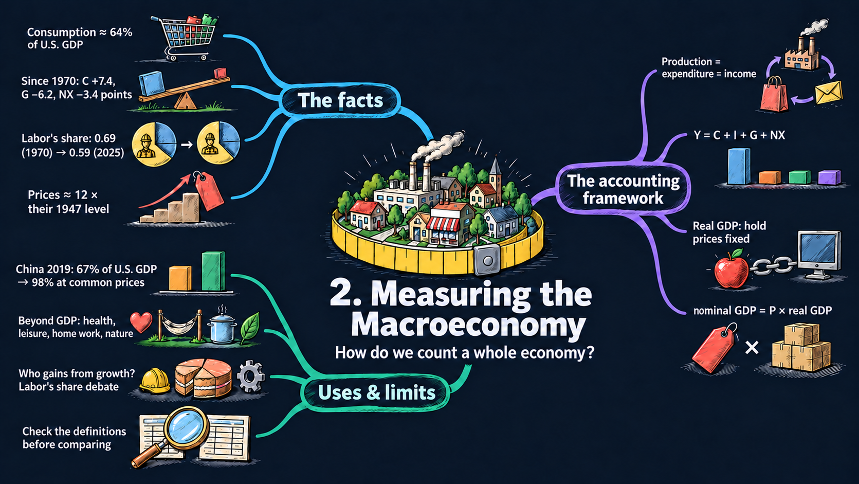
Learning goals

This chapter is about measurement: how economists turn millions of transactions into a few numbers that describe a whole economy. By the end of it you will be able to:

• derive why production = expenditure = income: value added adds up to final sales, and the national income identity \(Y = C + I + G + NX\) splits GDP by who buys it;
• describe how the composition of U.S. GDP and labor’s share of income have changed since 1929, and derive the labor-share measure that splits proprietors’ income;
• derive the Laspeyres, Paasche and chain-weighted growth rates of real GDP as weighted averages, and split nominal growth into inflation and real growth;
• compare GDP across countries with exchange rates and purchasing power parity, and read the comparative statics of each conversion;
• read CSV files with pandas, compute new columns, work with dates, and draw area and line charts with Plotly Express;
• compare countries, and check that two data sources use the same definitions before you compare them.

Model overview

Back on Islandia, the island country we met in Chapter 1, a small statistics office has a job to do every year: put one number on everything the island produced. Farms grow grain, mills grind it, bakeries sell bread, Harbor Boatworks builds boats, the Islandia Treasury hires teachers, and some goods arrive by ship from Mainland. How do the statisticians add all of that up without counting anything twice? How do they tell a richer year from a year in which only prices went up? And how can Islandia compare itself with Mainland, which pays in another currency? This section builds the accounting tools that answer these three questions, following Islandia’s statisticians step by step.

NoteThe big idea

The question. How do we turn millions of purchases and paychecks into a few numbers that describe a whole economy, and compare them across years and across countries?

The answer in one sentence. Gross domestic product (GDP), the market value of all final goods and services produced in a period, gives the same total whether we add up production, spending or income, and dividing it by the right price level turns it into real output that can be compared over time and between countries.

What goes in and what comes out. This chapter has no behavior to model and no parameters to choose. In go data: prices and quantities, producers’ sales and purchases, incomes, exchange rates and price levels. Out come is GDP and its shares, labor’s share of income, real GDP, the price level and inflation, and GDP at common prices.

Road map.

1. Production, expenditure and income: why the three ways of counting GDP agree, the national income identity and labor’s share.
2. Real GDP: quantity indexes and chain weighting: how to strip out price changes with the Laspeyres, Paasche and chained indexes.
3. Price indexes and inflation: how nominal growth splits into inflation and real growth.
4. Comparing countries: exchange rates and purchasing power parity: how to compare economies that use different currencies.
5. Model in code: the formulas as Python functions, checked with numbers, including Islandia’s apples and computers (Table 2.4).

Notation. A bar over a letter marks a parameter, a number we choose; this chapter has none. Every letter below is a variable measured in the data, which later chapters call endogenous once a model explains it. All the results of this section are identities: they hold in any data set because of the way the variables are defined, which makes them useful checks on the data.

Symbol	Meaning	Type
\(R_j, M_j, VA_j\)	revenue, purchased intermediate inputs and value added of producer \(j\)	endogenous
\(Y\)	GDP	endogenous
\(C, I, G\)	consumption, investment and government purchases	endogenous
\(X, IM, NX\)	exports, imports and net exports \(X - IM\)	endogenous
\(p_{i,t}, q_{i,t}\)	price and quantity of good \(i\) in year \(t\)	endogenous
\(s_{i,t}\)	share of good \(i\) in spending in year \(t\)	endogenous
\(P_t\)	price level of the whole economy (the GDP deflator)	endogenous
\(\pi\)	inflation rate, the growth rate of \(P_t\)	endogenous
\(e\)	exchange rate: units of the home currency per dollar	endogenous
\(t, i, j\)	year, good and producer	notation
\(g\), \(\Delta x\)	a growth rate, and the change in \(x\) between two years	notation

Production, expenditure and income

Definitions

• A final good ends up with its last user: a household, a firm that keeps it as capital, the government, or a buyer abroad. An intermediate good disappears into some other good made in the same period, like the grain in Islandia’s bread or the electricity that runs a mill.
• Producer \(j\) earns revenue \(R_j\) from its sales and pays \(M_j\) for the intermediate inputs it buys. The difference is its value added, the part of the value of its output that it created itself: \[VA_j \equiv R_j - M_j.\]
• Capital (buildings, machines, boats, software) helps to make output but is not used up within the period. Its wear and tear is called depreciation. GDP is gross because depreciation is not taken out; subtracting it gives net domestic product.
• Value added is paid out as income: compensation of employees (wages, salaries and benefits), taxes on production less subsidies, depreciation, and the net operating surplus, which goes to the owners. The operating surplus is whatever is left, so the four pieces always add up to value added.
• Spending on final goods comes in four parts: consumption \(C\); investment \(I\) (business structures, equipment, intellectual property products such as software and R&D, new housing, and the change in inventories); government purchases \(G\); and net exports \(NX\), exports \(X\) minus imports \(IM\). When the Islandia Treasury hires a teacher or buys a ferry, that is part of \(G\). When it pays a pension, or interest on its debt, it only moves income from some islanders to others and buys nothing, so that payment is not part of \(G\).
• Only new production counts. Selling a used boat a second time produces nothing new, but the dealer’s margin does count: it pays for the service of finding a buyer.

Deriving the results

Step 1: value added adds up to final sales. Picture a chain of \(J\) producers. The first buys no inputs, each one sells all of its output to the next, and the last one sells to final users. So \(M_1 = 0\) and \(M_j = R_{j-1}\), and

\[VA_1 = R_1, \qquad VA_2 = R_2 - R_1, \qquad \dots, \qquad VA_J = R_J - R_{J-1}.\]

Now add them up. Each revenue except the last shows up twice: with a plus sign as the seller’s revenue, and with a minus sign as the buyer’s cost. So the sum telescopes:

\[\sum_{j=1}^{J} VA_j = R_1 + (R_2 - R_1) + \dots + (R_J - R_{J-1}) = R_J.\]

The same cancellation works in any web of sales between firms, because each sale of an intermediate good is revenue for one firm and a cost for another. Counting production and counting final sales therefore give the same GDP:

\[\text{GDP} = \sum_j VA_j = \text{value of the final goods and services}.\]

TipIn words: count each stage once

If Islandia’s statisticians simply added up every firm’s sales, the grain inside a loaf of bread would be counted twice: once when the farm sells it to the mill, and again inside the price of the bread. Subtracting what each firm bought from other firms keeps only its own contribution, so every stage of the chain is counted exactly once.

Step 2: production = income. Add up the income split of value added over all producers:

\[\text{GDP} = \text{compensation} + \text{taxes on production less subsidies} + \text{net operating surplus} + \text{depreciation}.\]

Since the operating surplus is the leftover, every dollar of value added ends up as somebody’s income. In practice, though, statisticians measure income from other records (tax returns, payrolls) than the ones they use for spending. The income total is called gross domestic income (GDI), and the small gap between GDI and GDP is the statistical discrepancy.

Step 3: production = expenditure. Final goods are bought by households, firms, the government and foreigners. So buyers at home spend \(C + I + G\), and buyers abroad spend \(X\). Some of what \(C\), \(I\) and \(G\) buy, though, was made abroad and is not domestic production. Taking those imports out leaves the domestic output that went to final users: \(C + I + G + X - IM\). And goods that were made this year but not sold? They count as inventory investment, part of \(I\), as if the producer had bought its own output. So every unit produced has a buyer somewhere in the accounts:

\[Y = C + I + G + NX, \qquad NX \equiv X - IM.\]

This is the national income identity: GDP \(Y\) seen from the spending side.

ImportantKey result: GDP counted three ways

\[\text{GDP} = \sum_j VA_j = \text{value of the final goods and services} \tag{1}\]

\[Y = C + I + G + NX, \qquad NX \equiv X - IM \tag{2}\]

Equation (1): value added and final sales give the same total, which Step 2 shows is also paid out as income. Equation (2) splits it by buyer.

Islandia in numbers. An Islandia farm sells grain worth $40 to a mill, the mill sells flour worth $70 to a bakery, and the bakery sells bread worth $120 to islanders. The value added is \(40 + 30 + 50 = 120\), exactly the value of the bread. Adding up all sales would give \(230\).

Step 4: shares of GDP. Divide both sides of (2) by \(Y\) (Appendix C.2):

\[1 = \frac{C}{Y} + \frac{I}{Y} + \frac{G}{Y} + \frac{NX}{Y}.\]

The four shares sum to 100 percent in every year. Now compare two years. The left side is 1 in both, so its change is zero:

\[\Delta\frac{C}{Y} + \Delta\frac{I}{Y} + \Delta\frac{G}{Y} + \Delta\frac{NX}{Y} = 0.\]

If one share goes up, others must come down (Fig. 2). We compute shares from nominal values; the second block explains why.

Step 5: labor’s share of income. We want the part of income that pays for work. Two items belong neither clearly to labor nor clearly to capital. Taxes on production \(T\) (such as sales taxes) are nobody’s labor or capital income. Proprietors’ income \(\mathit{Prop}\), what the self-employed earn, pays both for their own work and for their own equipment, like an islander who fishes from a boat she owns. Income net of these taxes is

\[\text{GDI} - T = \text{compensation} + \mathit{Prop} + \text{other capital income}.\]

Assume that labor gets the same fraction of proprietors’ income as it gets of all other income, and call that fraction \(\theta\):

\[\theta = \frac{\text{compensation}}{\text{GDI} - T - \mathit{Prop}}, \qquad\text{so}\qquad \text{compensation} = \theta\,(\text{GDI} - T - \mathit{Prop}).\]

Labor’s total income is then compensation plus the fraction \(\theta\) of proprietors’ income. As a share of income net of taxes, it is

\[\frac{\text{compensation} + \theta\,\mathit{Prop}}{\text{GDI} - T} = \frac{\theta\,(\text{GDI} - T - \mathit{Prop}) + \theta\,\mathit{Prop}}{\text{GDI} - T} = \frac{\theta\,(\text{GDI} - T)}{\text{GDI} - T} = \theta.\]

So the labor share is \(\theta\):

ImportantKey result: labor’s share of income

\[\text{labor share} = \frac{\text{compensation}}{\text{GDI} - \text{taxes on production} - \text{proprietors' income}} \tag{3}\]

The capital share is one minus the labor share. Fig. 3 uses equation (3).

Islandia in numbers. Take round numbers for one year: GDI of 100, taxes on production of 7, proprietors’ income of 9 and compensation of 54 (in billions). Equation (3) gives a labor share of \(54/84 \approx 0.643\), while the simple ratio compensation/GDI is only \(0.54\).

TipIn words: the self-employed

We cannot tell which part of the fisher’s income pays for her work and which part pays for her boat. So we leave proprietors out of both the top and the bottom of the fraction. That gives the same answer as splitting their income in the same proportions as everybody else’s.

What the framework predicts

The identities say exactly which entries move when something happens. Some examples on Islandia, each worth \(\$p\):

Event	\(C\)	\(I\)	\(G\)	\(NX\)	GDP \(Y\)
An islander buys a new boat built by Harbor Boatworks	\(+p\)	0	0	0	\(+p\)
An islander buys a new boat built on Mainland	\(+p\)	0	0	\(-p\)	0
Harbor Boatworks builds a new workshop	0	\(+p\)	0	0	\(+p\)
Harbor Boatworks builds boats it cannot sell this year	0	\(+p\) (inventories)	0	0	\(+p\)
A Mainland buyer purchases a new boat built on Islandia	0	0	0	\(+p\)	\(+p\)
The Islandia Treasury pays a pension	0	0	0	0	0
The Islandia Treasury hires a teacher	0	0	\(+p\)	0	\(+p\)
A dealer resells a used boat with margin \(m\)	\(+m\)	0	0	0	\(+m\)

• Imports never add to GDP. An imported boat enters \(C\), \(I\) or \(G\) with a plus sign and \(NX\) with a minus sign, and the two cancel.
• The shares are tied together. They add up to one, so their changes add up to zero (Step 4). If the consumption share rises over a decade, some other share must have fallen to make room.
• GDP measures market production, not welfare. It leaves out work done at home (cooking, caring for one’s own children), the value of longer and healthier lives, leisure, and the using up of natural resources and harm to the environment. The note on Table 2.3 in the Fig. 3 section discusses a broader measure that adds some of them.

Production, spending and income are three views of one total, so each dollar of GDP is counted once and earned once.

NoteCheck your understanding

1. In Islandia’s chain, the mill now buys grain worth $40 and sells flour worth $80, and the bakery still sells bread worth $120. What is each producer’s value added, and what is GDP?

Answer

The farm adds 40, the mill \(80 - 40 = 40\) and the bakery \(120 - 80 = 40\). By equation (1), GDP is \(40 + 40 + 40 = 120\), the value of the bread. A higher price for flour moves value added from the bakery to the mill but leaves GDP unchanged.

2. An islander buys a new boat built on Mainland. Why does Islandia’s GDP not change?

Answer

The boat raises consumption \(C\) by its price, but it is also an import, so it lowers \(NX = X - IM\) by the same amount. In equation (2) the two changes cancel. The boat was produced on Mainland, so it is part of Mainland’s GDP, not Islandia’s.

Real GDP: quantity indexes and chain weighting

Definitions

Islandia produces goods \(i = 1, \dots, n\). Good \(i\) has price \(p_{i,t}\) and quantity \(q_{i,t}\) in year \(t\).

• Nominal GDP values each year’s goods at that same year’s prices: \(\text{nominal GDP}_t = \sum_i p_{i,t}\,q_{i,t}\).
• Real GDP at the prices of a base year \(b\) values each year’s goods at one fixed set of prices: \(\sum_i p_{i,b}\,q_{i,t}\). Since the prices never change, it moves only when the quantities move. It is measured in “year-\(b\) dollars”.
• The expenditure share of good \(i\) is \(s_{i,t} \equiv p_{i,t}q_{i,t}\big/\sum_k p_{k,t}q_{k,t}\). In every year the shares add up to one.
• The growth rate of the quantity of good \(i\) is \(g_i\), so \(q_{i,t+1} = (1+g_i)\,q_{i,t}\).

The price level, also called the GDP deflator, is defined as nominal GDP divided by real GDP, \(P_t \equiv \text{nominal GDP}_t/\text{real GDP}_t\). Multiply both sides by real GDP:

ImportantKey result: the price level links nominal and real GDP

\[\text{nominal GDP}_t = P_t \times \text{real GDP}_t \tag{4}\]

Real GDP tracks only quantities, and the price level \(P_t\) picks up the rest. If Islandia made just one good, \(P_t\) would be its price and real GDP its quantity. In the base year real and nominal GDP coincide, so \(P_b = 1\) (or 100, as an index).

Deriving the results

Step 1: two ways to hold prices fixed. To measure real growth from year \(t\) to year \(t+1\), we can value the quantities of both years at the starting prices (the Laspeyres index), or at the ending prices (the Paasche index):

\[1 + g^L = \frac{\sum_i p_{i,t}\,q_{i,t+1}}{\sum_i p_{i,t}\,q_{i,t}}, \qquad 1 + g^P = \frac{\sum_i p_{i,t+1}\,q_{i,t+1}}{\sum_i p_{i,t+1}\,q_{i,t}}.\]

Step 2: Laspeyres growth is an average of the goods’ growth rates. In the top of the fraction, write \((1+g_i)\,q_{i,t}\) for \(q_{i,t+1}\), and split the fraction into one term per good:

\[1 + g^L = \sum_i \frac{p_{i,t}\,q_{i,t}}{\sum_k p_{k,t}\,q_{k,t}}\,(1+g_i) = \sum_i s_{i,t}\,(1+g_i) = \sum_i s_{i,t} + \sum_i s_{i,t}\,g_i = 1 + \sum_i s_{i,t}\,g_i.\]

The last step uses the fact that the shares sum to one.

Step 3: Paasche growth is an average too, with other weights. Flip the Paasche fraction upside down and write \(q_{i,t+1}/(1+g_i)\) for \(q_{i,t}\):

\[\frac{1}{1+g^P} = \frac{\sum_i p_{i,t+1}\,q_{i,t}}{\sum_k p_{k,t+1}\,q_{k,t+1}} = \sum_i \frac{p_{i,t+1}\,q_{i,t+1}}{\sum_k p_{k,t+1}\,q_{k,t+1}}\cdot\frac{1}{1+g_i} = \sum_i \frac{s_{i,t+1}}{1+g_i}.\]

ImportantKey result: the two indexes as weighted averages

\[g^L = \sum_i s_{i,t}\,g_i, \qquad \frac{1}{1+g^P} = \sum_i \frac{s_{i,t+1}}{1+g_i} \tag{5}\]

Both indexes average the growth rates of the individual goods. Laspeyres weights each good by its share of spending in the first year. Paasche uses the shares of the last year, in the form of a weighted harmonic mean of the growth factors.

Islandia in numbers. Suppose Islandia makes only apples and computers, as in the textbook’s example. From 2026 to 2027 apples grow 10 percent and computers 20 percent. In 2026 computers take a share of about 0.833 of spending, so \(g^L = 0.167\times 10\% + 0.833 \times 20\% \approx 18.3\%\). At the 2027 prices the Paasche rate is about 17.7%.

TipIn words: why the two indexes disagree

The weights depend on prices. On Islandia, computers got cheaper relative to apples while their quantity grew faster. At the old prices computers were still expensive, so the Laspeyres index gives the fast-growing good a big weight and reports more growth. At the new prices computers weigh less, and the Paasche index reports less.

When do the two agree? (a) If every quantity grows at the same rate \(g\), both formulas in (5) give exactly \(g\), since the shares sum to one. (b) If every price changes by the same factor \(\lambda\), so that \(p_{i,t+1} = \lambda p_{i,t}\), then \(\lambda\) cancels from the top and the bottom of the Paasche fraction, and it turns into the Laspeyres fraction. So the two indexes can differ only when relative prices change. Usually the goods whose relative price falls, like computers, are also the goods whose quantity grows fastest. At the starting prices those goods are still expensive and carry a large weight, so \(g^L > g^P\). The longer the period, the more relative prices change, and the wider the gap.

Step 4: chain weighting. The chain-weighted index splits the difference and averages the two growth rates:

\[g^{\text{chain}} = \tfrac{1}{2}\left(g^L + g^P\right).\]

ImportantKey result: chain-weighted growth

\[g^{\text{chain}} = \tfrac{1}{2}\left(g^L + g^P\right) \tag{6}\]

Statistical agencies use the Fisher index, the geometric mean of the two growth factors, \(1 + g^F = \sqrt{(1+g^L)(1+g^P)}\). When the two rates are close, the two kinds of average are practically the same (Appendix C.6); the code below compares them.

Islandia in numbers. Averaging 18.3% and 17.7% gives chain-weighted growth of about 18.0% from 2026 to 2027.

Step 5: linking the years into a chain. Equation (6) is applied to each pair of neighboring years, so the weights are always the prices of those two years. To get levels from the growth rates, choose a benchmark year \(b\) in which real GDP is set equal to nominal GDP. Then step forward and backward one year at a time:

\[X_{t+1} = X_t\,(1 + g^{\text{chain}}_{t,t+1}), \qquad X_t = \frac{X_{t+1}}{1 + g^{\text{chain}}_{t,t+1}},\]

where \(X_t\) is chained real GDP. Across several years the growth factors multiply, \(X_T = X_b\,(1+g_{b,b+1})(1+g_{b+1,b+2})\cdots(1+g_{T-1,T})\). The levels are reported in “chained year-\(b\) dollars”.

What the framework predicts

From year \(t\) to \(t+1\) …	Nominal GDP	Laspeyres \(g^L\)	Paasche \(g^P\)	Chained \(g^{\text{chain}}\)	Price level \(P\)
every price \(\times\lambda\), same quantities	\(\times\lambda\)	0	0	0	\(\times\lambda\)
every quantity \(\times\mu\), same prices	\(\times\mu\)	\(\mu-1\)	\(\mu-1\)	\(\mu-1\)	unchanged
relative prices change, same quantities	changes	0	0	0	moves with nominal GDP
quantities grow fastest where relative prices fall	rises	highest	lowest	in between

• Real GDP ignores pure price changes. When only prices move, every index reports zero real growth, and the whole change in nominal GDP lands in the price level.
• Fixed base years go out of date. Over long spans the Laspeyres index overstates growth and the Paasche index understates it. The U.S. national accounts moved to chain weighting in the 1990s, a time of fast-falling computer prices.
• Chained components do not add up. Each chained component has its own weights, so chained \(C + I + G + NX\) is generally not equal to chained GDP. For shares, use nominal values, which do add up (equation 2). For real growth rates, use chained real values.

Real GDP holds prices fixed so that only quantities move, and chain weighting keeps those prices up to date.

NoteCheck your understanding

1. One year every price on Islandia doubles, and every quantity stays the same. What happens to nominal GDP, to real growth by each index, and to the price level?

Answer

Nominal GDP doubles. Relative prices do not change, so the Laspeyres, Paasche and chained indexes all report zero real growth (the first row of the table). By equation (4), the price level doubles: the whole change in nominal GDP is a change in prices.

2. Islandia’s computers grew 20 percent and its apples 10 percent. Without computing anything, why must every index of real growth lie between these two numbers?

Answer

By equation (5), the Laspeyres and Paasche rates are weighted averages of the goods’ growth rates, with weights that are positive and sum to one. An average can never be larger than the largest item or smaller than the smallest. The chained rate of equation (6) averages the two again, so it lies in the same range.

Price indexes and inflation

Definitions

• The GDP deflator is the price level of equation (4), \(P_t = \text{nominal GDP}_t/\text{real GDP}_t\), usually multiplied by 100 so that it equals 100 in the base year.
• The inflation rate is the growth rate of the price level, \(\pi_{t+1} \equiv P_{t+1}/P_t - 1\).
• Each quantity index has a twin price index. The Laspeyres price index prices the starting quantities at both years’ prices, \(\sum_i p_{i,t+1}q_{i,t}\big/\sum_i p_{i,t}q_{i,t}\). The Paasche price index uses the ending quantities, \(\sum_i p_{i,t+1}q_{i,t+1}\big/\sum_i p_{i,t}q_{i,t+1}\).

Deriving the results

Step 1: nominal growth splits exactly into a price part and a quantity part. Multiply and divide the growth factor of nominal GDP by \(\sum_i p_{i,t}q_{i,t+1}\):

\[\frac{\sum_i p_{i,t+1}q_{i,t+1}}{\sum_i p_{i,t}q_{i,t}} = \underbrace{\frac{\sum_i p_{i,t+1}q_{i,t+1}}{\sum_i p_{i,t}q_{i,t+1}}}_{\text{Paasche price index}} \times \underbrace{\frac{\sum_i p_{i,t}q_{i,t+1}}{\sum_i p_{i,t}q_{i,t}}}_{\text{Laspeyres quantity index}}.\]

Multiplying and dividing by \(\sum_i p_{i,t+1}q_{i,t}\) instead gives the Laspeyres price index times the Paasche quantity index. Multiply the two splits together and take the square root: the Fisher price index times the Fisher quantity index is also exactly the growth factor of nominal GDP. That is why a chained price index and chained real GDP always satisfy equation (4).

Step 2: the growth rate of a product. Write equation (4) for two neighboring years and divide one by the other. The growth factor of a product is the product of the growth factors:

\[1 + g_{\text{nominal}} = (1+\pi)(1+g_{\text{real}}) = 1 + \pi + g_{\text{real}} + \pi\,g_{\text{real}}.\]

Take 1 away from both sides: \(g_{\text{nominal}} = \pi + g_{\text{real}} + \pi\,g_{\text{real}}\). The last term multiplies two small numbers, so it is much smaller than the others. Dropping it (Appendix C.5) leaves

\[g_{\text{nominal GDP}} \approx \pi + g_{\text{real GDP}}.\]

ImportantKey result: nominal growth = inflation + real growth

\[g_{\text{nominal GDP}} \approx \pi + g_{\text{real GDP}} \tag{7}\]

To get inflation from the other two, solve the exact form for \(\pi\): \(\pi = (1+g_{\text{nominal}})/(1+g_{\text{real}}) - 1 \approx g_{\text{nominal}} - g_{\text{real}}\). In natural logs the split is exact: \(\ln(\text{nominal GDP}) = \ln P + \ln(\text{real GDP})\), so the changes in logs add up with no error (Appendix C.4).

Islandia in numbers. From 2026 to 2027 Islandia’s nominal GDP grows 27.5% and chained real GDP 18.0%. The rule of thumb puts inflation at \(27.5 - 18.0 = 9.5\) percent, but the exact formula gives about 8.0%.

TipIn words: more expensive goods, or more goods

Islandia’s nominal GDP can grow because each apple and each computer costs more, or because there are more apples and computers. Equation (7) simply adds the two sources. The small cross term it leaves out is the price increase on the extra goods.

Step 3: rates over different periods. With quarterly data, the change from a year ago compares a quarter with the same quarter one year before, \(P_t/P_{t-4} - 1\). A one-quarter change becomes an annual rate by compounding it four times, \((P_t/P_{t-1})^4 - 1\), which is close to four times the quarterly rate when that rate is small (Appendix C.3). Over \(T\) years, the average annual growth rate \(\bar{g}\) is the constant rate that carries the first value to the last: \(P_T = P_0(1+\bar{g})^T\). Raise both sides of \(P_T/P_0 = (1+\bar{g})^T\) to the power \(1/T\) and subtract 1:

\[\bar{g} = \left(\frac{P_T}{P_0}\right)^{1/T} - 1.\]

(Here the bar marks an average over the years, not a parameter.)

Step 4: changing the base year. Rebasing an index to year \(b\) means \(P'_t = 100 \times P_t/P_b\). The constant \(100/P_b\) cancels in every ratio, \(P'_{t+1}/P'_t = P_{t+1}/P_t\), so rebasing shifts the level of the index but leaves every growth rate and inflation rate as it was.

What the framework predicts

Take the change in logs of equation (4), \(\Delta\ln(\text{nominal GDP}) = \Delta\ln P + \Delta\ln(\text{real GDP})\): the elasticity of nominal GDP with respect to the price level is 1, and with respect to real GDP it is also 1.

If …	then …
inflation is 1 point higher and real growth is unchanged	nominal growth is about 1 point higher
nominal growth is unchanged and real growth is 1 point higher	measured inflation is about 1 point lower
an index is rebased	its level changes; growth rates and inflation do not

• The rule of thumb in equation (7) works well when rates are small. With 2 percent inflation and 2 percent real growth, the cross term is only \(0.02 \times 0.02 = 0.0004\), or 0.04 percentage points. In Islandia’s apples-and-computers example, with prices up 8 percent and quantities up 18 percent, it is about 1.5 points (see the checks below). In a country with very high inflation it can be large.
• Ratio scales show inflation directly. Since \(\ln P_t\) rises by about \(\pi\) each year, constant inflation draws a straight line on a ratio (log) scale (Fig. 4).

Nominal growth is roughly inflation plus real growth; the small cross term matters only when rates are large.

NoteCheck your understanding

1. Islandia’s nominal GDP grows 5 percent in a year and its real GDP 3 percent. What is inflation by the rule of thumb, and what is it exactly?

Answer

By equation (7), \(\pi \approx 5 - 3 = 2\) percent. The exact form gives \(\pi = 1.05/1.03 - 1 \approx 1.94\%\). With rates this small the cross term is tiny, so the rule of thumb is close.

2. Islandia’s price level doubles over 10 years. What is the average annual inflation rate, and why is it not simply 10 percent?

Answer

By Step 3, \(\bar{g} = 2^{1/10} - 1 \approx 7.18\%\) a year. Ten years at 10 percent would multiply prices by \(1.1^{10} \approx 2.59\), not by 2, because each year’s increase builds on the higher prices of the year before.

Comparing countries: exchange rates and purchasing power parity

Definitions

Islandia’s statisticians will also ask whether their island is richer or poorer than Mainland, which uses a different currency. The tools are the same for any pair of countries. We write them for the textbook’s pair, China and the United States, and use its numbers.

• The exchange rate \(e\) is the number of yuan that buy one dollar in the currency market.
• China’s GDP in its own currency is \(Y^{\text{yuan}}\). Converted at the exchange rate, it is \(\text{nominal GDP}^{\text{dollars}}_{\text{China}} = Y^{\text{yuan}}/e\).
• \(\text{price level}_{\text{U.S.}}\) and \(\text{price level}_{\text{China}}\) are the cost of the same basket of goods in each country, both in dollars at the exchange rate. Their ratio, the relative price level, says how expensive China is compared with the United States.
• The PPP conversion factor is the number of yuan that buy in China what one dollar buys in the United States: \(\text{PPP} = e \times \text{price level}_{\text{China}}/\text{price level}_{\text{U.S.}}\).

Deriving the results

Step 1: China’s real output. Equation (4) holds in China too, with every value in dollars. Solve it for real GDP:

\[\text{real GDP}_{\text{China}} = \frac{\text{nominal GDP}^{\text{dollars}}_{\text{China}}}{\text{price level}_{\text{China}}}.\]

Step 2: value China’s goods at U.S. prices. To compare like with like, we price China’s quantities at the prices that hold in the United States:

\[\text{real GDP}^{\text{U.S. prices}}_{\text{China}} = \text{price level}_{\text{U.S.}} \times \text{real GDP}_{\text{China}}.\]

Step 3: substitute Step 1 into Step 2.

\[\text{real GDP}^{\text{U.S. prices}}_{\text{China}} = \frac{\text{price level}_{\text{U.S.}}}{\text{price level}_{\text{China}}} \times \text{nominal GDP}^{\text{dollars}}_{\text{China}}.\]

ImportantKey result: GDP at common prices

\[\text{real GDP}^{\text{U.S. prices}}_{\text{China}} = \frac{\text{price level}_{\text{U.S.}}}{\text{price level}_{\text{China}}} \times \text{nominal GDP}^{\text{dollars}}_{\text{China}} \tag{8}\]

Dollar GDP is divided by China’s relative price level. Where goods are cheap, the same dollars stand for more goods.

In numbers. With the textbook’s 2019 data, 95.1 trillion yuan at 6.91 yuan per dollar is about $13.8 trillion, 67 percent of U.S. GDP of $20.6 trillion. Chinese prices are 68.4 percent of U.S. prices, so at U.S. prices China’s GDP is about $20.1 trillion, 98 percent of U.S. GDP.

TipIn words: cheap haircuts

Suppose a haircut on Islandia costs half of what it costs on Mainland. Converting Islandia’s GDP at the exchange rate counts each Islandia haircut as half a Mainland haircut, even though it is the same service. Valuing both islands’ goods at the same prices fixes this, and it raises the measured output of the cheaper place.

Step 4: the shortcut through the PPP factor. Put \(\text{nominal GDP}^{\text{dollars}}_{\text{China}} = Y^{\text{yuan}}/e\) into (8) and gather the terms in the denominator:

\[\text{real GDP}^{\text{U.S. prices}}_{\text{China}} = \frac{Y^{\text{yuan}}}{e \times \text{price level}_{\text{China}}/\text{price level}_{\text{U.S.}}} = \frac{Y^{\text{yuan}}}{\text{PPP}}.\]

So we can bypass the exchange rate entirely: GDP in yuan divided by the PPP conversion factor is GDP at U.S. prices.

Step 5: how much of the gap is due to prices? Divide (8) by U.S. GDP and take logs (Appendix C.4):

\[\ln\frac{\text{real GDP}^{\text{U.S. prices}}_{\text{China}}}{\text{GDP}_{\text{U.S.}}} = \ln\frac{\text{nominal GDP}^{\text{dollars}}_{\text{China}}}{\text{GDP}_{\text{U.S.}}} - \ln\frac{\text{price level}_{\text{China}}}{\text{price level}_{\text{U.S.}}}.\]

The log gap at common prices is the log gap at the exchange rate minus the log of the relative price level. When China is cheaper, that log is negative, and the gap at common prices is smaller. Dividing both GDPs by population gives the same split for GDP per person.

Pricing China’s goods at U.S. prices is the cross-country cousin of a Laspeyres index; pricing U.S. goods at Chinese prices would be the Paasche version. In practice, the World Bank’s International Comparison Program and the Penn World Table use average world prices (“international dollars”), much as chain weighting averages the two indexes over time.

What the framework predicts

A 1% rise in …	GDP at the exchange rate	GDP at common prices	Relative price level of China
the exchange rate \(e\) (a weaker yuan), with yuan prices unchanged	\(-1\%\)	0	\(-1\%\)
every yuan price in China, with quantities unchanged	\(+1\%\)	0	\(+1\%\)
China’s output of every good	\(+1\%\)	\(+1\%\)	0

• Common prices do not react to the currency market. A swing in the exchange rate moves GDP in dollars one for one, but leaves the comparison at common prices where it was, because China’s goods get cheaper in dollars by the same 1 percent (the elasticity of dollar GDP with respect to \(e\) is \(-1\)).
• Rich countries look less far ahead at common prices. Services that cannot be traded, such as haircuts or restaurant meals, take a lot of labor, so they are cheap where wages are low. Poor countries therefore have low price levels, and comparisons at exchange rates exaggerate the income gaps between rich and poor countries.

To compare countries, value their goods at the same prices; exchange rates alone make cheap countries look poorer than they are.

NoteCheck your understanding

1. Suppose that at the exchange rate Islandia’s GDP is 40 percent of Mainland’s, and that goods on Islandia cost 80 percent of what they cost on Mainland. How large is Islandia’s GDP at Mainland’s prices, as a share of Mainland’s GDP?

Answer

By equation (8), divide the share at the exchange rate by the relative price level: \(40/0.8 = 50\) percent. Because Islandia is cheaper, the gap shrinks from 60 to 50 percentage points.

2. Islandia’s currency loses value against Mainland’s, while nothing else changes on either island. What happens to Islandia’s GDP at the exchange rate and at common prices?

Answer

At the exchange rate, Islandia’s GDP falls in Mainland’s currency, one for one with the currency (the first row of the table). At common prices nothing changes: the same goods are produced, and Islandia’s relative price level falls by exactly as much, so the two effects cancel in equation (8).

NoteRecap

• One total, three ways: value added, final spending and income all add up to GDP, equations (1) and (2); the spending shares move together (Fig. 2).
• Labor’s share leaves taxes and proprietors’ income out of the denominator, equation (3) (Fig. 3).
• Real GDP values quantities at fixed prices; Laspeyres and Paasche are weighted averages of the goods’ growth rates, and chain weighting averages the two, equations (5) and (6).
• Prices and inflation: nominal GDP is the price level times real GDP, equation (4), and nominal growth is about inflation plus real growth, equation (7) (Fig. 4; Fig. 5 plots the inflation rate).
• Comparing countries needs common prices, equation (8): at exchange rates, poor countries look poorer than they are (Comparing countries).

Model in code

Now we turn the measurement rules into Python. The section has three parts: the setup (folded, because it is nearly the same in every chapter), the rules as functions, and numerical checks of the Key results, from Islandia’s bakery to China at common prices. Run its cells once, in order. Every later section of the notebook reuses them.

Setup

Run the setup cells once, before anything else. They load the Python libraries, give every chart the same look, store the address of the chapter’s data and define four helpers that only the book website needs. You can use the notebook without reading them; open the box if you are curious.

NoteShow the setup code

The first cell loads the libraries and sets the look of the charts. Its comments explain each step.

# @title Setup: libraries, chart colors and the data location
# Text after a "#" is a comment: Python ignores it, it is there for human readers.

# Step 1: load the libraries. `import` loads a library, a toolbox written by
# other people, and `as pd` gives pandas the short nickname pd, so the code stays short.
import numpy as np                    # numbers and arrays
import pandas as pd                   # data tables
import plotly.express as px           # quick charts from data tables
import plotly.graph_objects as go     # charts built piece by piece
import plotly.io as pio               # settings shared by every chart
# menus, buttons and sliders for the interactive figures
from ipywidgets import interact, ToggleButtons, Dropdown, SelectMultiple, FloatSlider, IntSlider

# Step 2: one light blue/green look for every chart
BLUE, TEAL, GREEN, GRAY = "#16528c", "#008070", "#7fb23a", "#8a96a3"
pio.templates.default = "plotly_white"
# the same chart size in Colab and on the website
pio.templates["plotly_white"].layout.update(width=860, height=480)
px.defaults.color_discrete_sequence = [BLUE, TEAL, GREEN, "#5aa0d8", "#0b4f47", "#e0a33b"]
WIDE = {"description_width": "initial"}         # show the full widget labels

# Step 3, Colab only: let Plotly charts appear inside the interactive widgets.
# `try` runs the indented lines; if the import fails (we are not in Colab),
# `except` skips them.
try:
    import google.colab
    google.colab.output.enable_custom_widget_manager()
except ImportError:
    pass                                        # not running in Colab: nothing to do

# Step 4: the data files of this chapter live in the book's GitHub repository
DATA_URL = "https://raw.githubusercontent.com/quarcs-lab/macro102-site/main/data/ch02/"

The website cannot run Python, so each interactive figure also gets a version with a precomputed slider or menu. The next helpers build those versions. Run them and move on.

# @title Helper for the website versions (run this cell; you do not need to read it)
def slider_figure(make_figure, name, values, start, label=None):
    """Join precomputed versions of a figure with one slider (the website cannot run Python).

    Arguments
        make_figure : the function that draws the figure, e.g. changes_chart
        name        : the argument the slider moves, e.g. "base_year"
        values      : the values of that argument to precompute
        start       : the value shown first
        label       : the slider's label (the argument name if None)
    Returns
        one Plotly figure with all versions and a slider that shows one at a time
    """
    # Step 1: draw the figure once for every value
    figures = [make_figure(**{name: v}) for v in values]
    first = values.index(start)
    # Step 2: copy every curve into one figure; only the start value's are visible
    fig = go.Figure(layout=figures[first].layout)
    owner = []                          # which precomputed figure each trace is from
    for i, f in enumerate(figures):
        for trace in f.data:
            trace.visible = (i == first)
            fig.add_trace(trace)
            owner.append(i)
    # Step 3: one slider step per value: its curves, title, labels and shapes
    steps = []
    for i, f in enumerate(figures):
        layout = {"title": f.layout.title.to_plotly_json(),
                  "annotations": [a.to_plotly_json() for a in f.layout.annotations],
                  "shapes": [s.to_plotly_json() for s in f.layout.shapes]}
        visible = [o == i for o in owner]
        steps.append(dict(method="update", label=str(values[i]), args=[{"visible": visible}, layout]))
    fig.update_layout(sliders=[dict(active=first, steps=steps, pad=dict(t=60),
                                    currentvalue=dict(prefix=(label or name) + " = "))])
    return fig

The data figures of this chapter let you add other countries. On the website, a menu above each of these figures adds a group of countries (the G7, a world region, …); the next cell builds those menus.

# @title Helpers for the website's country menus (run this cell; you do not need to read it)
def country_traces(data, y, skip, x="year", fmt=".1f", markers=False):
    """One line per country of a long table, leaving out the countries in `skip`.

    Arguments
        data    : a long table with one row per country and year (columns country, x, y)
        y       : the column to draw
        skip    : the countries to leave out
        x       : the column on the horizontal axis
        fmt     : the number format of the hover text, e.g. ".1f"
        markers : True to draw a dot at every point of the line
    Returns
        a dictionary: each country's name and its list of traces (one line in its color)
    """
    # Step 1: go through the table one country at a time
    extra = {}
    for name, part in data.groupby("country"):
        if name not in skip:
            # Step 2: one line for this country, in its COLORS color, with hover text
            extra[name] = [go.Scatter(x=part[x], y=part[y], name=name,
                                      mode="lines+markers" if markers else "lines",
                                      line=dict(color=COLORS[name], width=2),
                                      hovertemplate=f"<b>{name}</b><br>%{{x}}: %{{y:{fmt}}}<extra></extra>")]
    return extra


def country_menu(fig, extra, countries):
    """Add the extra countries' lines hidden, and a menu that shows one group of them.

    The groups are the G7, the G20, the OECD and each world region. The traces already in
    fig (the textbook's) stay as they are, and the slider steps only switch those.

    Arguments
        fig       : a Plotly figure with the textbook's countries
        extra     : the other countries' lines, from country_traces
        countries : a table with one row per country (columns country, region, g7, g20, oecd)
    Returns
        the same figure, with the extra lines hidden and the group menu above the plot
    """
    # Step 1: add every extra line, hidden, and remember whose line it is
    n = len(fig.data)                           # the number of textbook traces
    owner = []
    for name, traces in extra.items():
        for trace in traces:
            trace.visible = False
            fig.add_trace(trace)
            owner.append(name)
    # Step 2: the groups of the menu: G7, G20, OECD, then each region, A to Z
    groups = {"G7": countries.country[countries.g7], "G20": countries.country[countries.g20],
              "OECD": countries.country[countries.oecd]}
    for region in sorted(countries.region.unique()):
        groups[region] = countries.country[countries.region == region]
    # Step 3: one button per group; each switches only the extra lines, `rest`
    rest, autoscale = list(range(n, len(fig.data))), {"yaxis.autorange": True}
    buttons = [dict(label="Textbook only", method="update",
                    args=[{"visible": [False] * len(owner)}, autoscale, rest])]
    for label, members in groups.items():
        visible = [o in set(members) for o in owner]
        # leave out a group with no country in the data
        if any(visible):
            buttons.append(dict(label=f"+ {label} ({sum(visible)})", method="update",
                                args=[{"visible": visible}, autoscale, rest]))
    # Step 4: put the menu above the plot, at the right
    menu = dict(type="dropdown", buttons=buttons, active=0, x=1, xanchor="right", y=1.02, yanchor="bottom")
    fig.update_layout(updatemenus=list(fig.layout.updatemenus) + [menu], margin=dict(t=110))
    # Step 5: make every slider step switch only the textbook traces, the first n
    for slider in fig.layout.sliders:
        for step in slider.steps:
            step.args = [{"visible": list(step.args[0]["visible"])}, step.args[1], list(range(n))]
    return fig

The last helper is like slider_figure, but with a dropdown menu, for the figures that show one country at a time.

# @title Helper for the website's one-country menus (run this cell; you do not need to read it)
def dropdown_figure(make_figure, name, values, start):
    """Like slider_figure, but with a dropdown menu: one precomputed figure per value.

    Arguments
        make_figure : the function that draws the figure, e.g. composition_chart
        name        : the argument the menu sets, e.g. "country"
        values      : the values of that argument to precompute (e.g. the countries)
        start       : the value shown first
    Returns
        one Plotly figure with all versions and a menu that shows one at a time
    """
    # Step 1: draw the figure once for every value
    figures = [make_figure(**{name: v}) for v in values]
    fig = go.Figure(layout=figures[values.index(start)].layout)
    # Step 2: copy every trace into one figure; only the start value's are visible
    owner = []
    for i, f in enumerate(figures):
        for trace in f.data:
            trace.visible = (values[i] == start)
            fig.add_trace(trace)
            owner.append(i)
    # Step 3: one menu entry per value: its traces, title, labels, shapes and axes
    buttons = []
    for i, f in enumerate(figures):
        layout = {"title": f.layout.title.to_plotly_json(),
                  "annotations": [a.to_plotly_json() for a in f.layout.annotations],
                  "shapes": [s.to_plotly_json() for s in f.layout.shapes],
                  "yaxis": f.layout.yaxis.to_plotly_json(),
                  "xaxis": f.layout.xaxis.to_plotly_json()}
        # a second vertical axis (Fig. 2)
        if "yaxis2" in f.layout.to_plotly_json():
            layout["yaxis2"] = f.layout.yaxis2.to_plotly_json()
        buttons.append(dict(label=str(values[i]), method="update",
                            args=[{"visible": [o == i for o in owner]}, layout]))
    # Step 4: put the menu above the plot, at the right
    menu = dict(type="dropdown", buttons=buttons, active=values.index(start), x=1, xanchor="right", y=1.02,
                yanchor="bottom")
    fig.update_layout(updatemenus=[menu], margin=dict(t=110))
    return fig

The model as functions

This chapter has no behavior to model, but its measurement rules are formulas, and we write each one as a Python function: a named recipe that takes inputs and gives back a result. The first three are shares, the value of production, and chain-weighted growth, equation (6).

# `def` creates a function. Its inputs are the arguments in parentheses, and
# `return` gives back the result. The text in triple quotes describes the function.
def share(part, total):
    """Share of a part in a total, in percent.

    Tables 2.1 and 2.2, and the shares of equation (2):  share = 100 * part / total

    Arguments
        part  : the part, e.g. consumption or compensation
        total : the total, e.g. GDP
    Returns
        the share of the part in the total, in percent
    """
    return 100 * part / total


def gdp_value(prices, quantities):
    """Value of production: price times quantity, added over all goods.

    Equation (4) and the indexes of equation (5) use it:  value = sum over i of p_i * q_i
    With each year's own prices it is nominal GDP; with fixed prices, real GDP.

    Arguments
        prices     : the price of each good, p_i
        quantities : the quantity of each good, q_i
    Returns
        the value of production, in dollars
    """
    # multiply good by good; `.sum()` adds up all the values of a column or a row
    return (prices * quantities).sum()


def chain_growth(g_laspeyres, g_paasche):
    """Chain-weighted growth of real GDP.

    Equation (6):  g_chain = (g_L + g_P) / 2

    Arguments
        g_laspeyres : the Laspeyres growth rate, g_L (at the starting prices)
        g_paasche   : the Paasche growth rate, g_P (at the ending prices)
    Returns
        the chain-weighted growth rate, g_chain
    """
    # the simple average of the two growth rates
    return (g_laspeyres + g_paasche) / 2

The last two functions compare countries. One converts GDP into dollars at the market exchange rate, and the other values it at U.S. prices, equation (8).

def to_dollars(gdp_local, exchange_rate):
    """GDP in dollars at the market exchange rate.

    The first step of equation (8):  GDP in dollars = GDP in local currency / e

    Arguments
        gdp_local     : GDP in the local currency, e.g. trillions of yuan
        exchange_rate : the exchange rate e, units of local currency per dollar
    Returns
        GDP in dollars
    """
    return gdp_local / exchange_rate


def at_common_prices(gdp_dollars, relative_price_level):
    """Real GDP at U.S. prices.

    Equation (8):  real GDP at U.S. prices = GDP in dollars / (price level / U.S. price level)

    Arguments
        gdp_dollars          : GDP in dollars, from to_dollars
        relative_price_level : the country's price level relative to the U.S. (U.S. = 1)
    Returns
        real GDP at U.S. prices, in dollars
    """
    # where goods are cheap (a relative price level below 1), the same dollars buy more
    return gdp_dollars / relative_price_level

Checking the key results

The rules came from algebra. Now we check them with numbers, one Key result at a time, mostly with small made-up examples from Islandia.

Check 1: value added adds up to final sales (equation 1). Islandia’s chain of three producers: a farm grows grain worth $40 and sells it to a mill; the mill turns it into flour worth $70 and sells it to a bakery; the bakery sells bread worth $120 to islanders.

# Step 1: each producer's sales and purchases. `pd.Series({...})` builds one
# labeled column from a dictionary: the keys become the labels.
revenue = pd.Series({"farm": 40, "mill": 70, "bakery": 120})
# each buys the output of the one before
inputs = pd.Series({"farm": 0, "mill": 40, "bakery": 70})
# Step 2: value added; subtracting two Series subtracts the values with the same label
value_added = revenue - inputs
print(value_added)
# Step 3: equation (1): the sum of value added equals the final sales
print(f"Sum of value added:   ${value_added.sum()}")
print(f"Final sales (bread):  ${revenue['bakery']}")
print(f"Sum of all revenues:  ${revenue.sum()}   (counts the grain three times and the flour twice)")

farm      40
mill      30
bakery    50
dtype: int64
Sum of value added:   $120
Final sales (bread):  $120
Sum of all revenues:  $230   (counts the grain three times and the flour twice)

Check 2: the labor share (equation 3). We take made-up round numbers for one year’s income on Islandia (in billions) and check the algebra of Step 5: splitting proprietors’ income in the economy-wide proportion gives the same labor share as leaving it out of the fraction.

# Step 1: Islandia's income in one year, in billions
gdi, taxes, proprietors, compensation = 100.0, 7.0, 9.0, 54.0
# Step 2: the labor share in two ways
theta = compensation / (gdi - taxes - proprietors)                  # equation (3)
# proprietors' income split by theta
split = (compensation + theta * proprietors) / (gdi - taxes)
# Step 3: both give the same share; compensation / GDI alone is too low
print(f"Labor share, equation (3):                 {theta:.4f}")
print(f"Labor share with proprietors split:        {split:.4f}")
print(f"Simple share, compensation / GDI:          {compensation / gdi:.4f}   (lower)")

Labor share, equation (3):                 0.6429
Labor share with proprietors split:        0.6429
Simple share, compensation / GDI:          0.5400   (lower)

Check 3: real GDP in the economy of Table 2.4. In this example Islandia produces only apples and computers, as in the textbook’s Table 2.4. We store its prices and quantities in two small tables, one row per year.

# Prices and quantities of the two goods, one row per year.
# `pd.DataFrame({...}, index=[...])` builds a table from a dictionary: each key
# becomes a column, and the `index` gives the row labels.
prices = pd.DataFrame({"apples": [1, 2, 3], "computers": [900, 1000, 1000]}, index=[2025, 2026, 2027])
quantities = pd.DataFrame({"apples": [500, 500, 550], "computers": [5, 5, 6]}, index=[2025, 2026, 2027])
prices

	apples	computers
2025	1	900
2026	2	1000
2027	3	1000

Nominal GDP uses each year’s own prices. Real GDP holds the prices fixed. The Laspeyres index measures the change from 2026 to 2027 with the initial (2026) prices, and the Paasche index with the final (2027) prices. Chain weighting averages the two growth rates (equation 6).

# Step 1: nominal GDP, each year at its own prices. `prices.loc[2026]` picks the
# row for 2026. An f-string, f"... {x:,.0f}", puts a value into the text: ","
# adds thousands separators, ".0f" shows no decimals, ".1%" a percentage.
for year in [2025, 2026, 2027]:
    print(f"Nominal GDP in {year}: ${gdp_value(prices.loc[year], quantities.loc[year]):,.0f}")

# Step 2: growth 2026-2027, nominal and at fixed prices; multiplying two rows,
# `prices.loc[2026] * quantities.loc[2027]`, multiplies the matching columns
g_nominal = gdp_value(prices.loc[2027], quantities.loc[2027]) / gdp_value(prices.loc[2026], quantities.loc[2026]) - 1
# Laspeyres: at the 2026 prices; Paasche: at the 2027 prices
g_laspeyres = gdp_value(prices.loc[2026], quantities.loc[2027]) / gdp_value(prices.loc[2026], quantities.loc[2026]) - 1
g_paasche = gdp_value(prices.loc[2027], quantities.loc[2027]) / gdp_value(prices.loc[2027], quantities.loc[2026]) - 1
g_chain = chain_growth(g_laspeyres, g_paasche)              # equation (6)
# Step 3: the numbers of Table 2.4
print(f"Real GDP in 2027 at 2026 prices: ${gdp_value(prices.loc[2026], quantities.loc[2027]):,.0f}")
print(f"Real GDP in 2026 at 2027 prices: ${gdp_value(prices.loc[2027], quantities.loc[2026]):,.0f}")
print(f"Growth 2026-2027: nominal {g_nominal:.1%}, Laspeyres {g_laspeyres:.1%}, "
      f"Paasche {g_paasche:.1%}, chain-weighted {g_chain:.1%}")
# Step 4: chained real GDP in 2026, going back one year from 2027 (nominal GDP $7,650)
print(f"Chained real GDP in 2026, benchmarked to 2027: ${7650 / (1 + g_chain):,.0f}")
# the rule of thumb of equation (7)
print(f"Inflation (nominal growth minus real growth):  {g_nominal - g_chain:.1%}")

Nominal GDP in 2025: $5,000
Nominal GDP in 2026: $6,000
Nominal GDP in 2027: $7,650
Real GDP in 2027 at 2026 prices: $7,100
Real GDP in 2026 at 2027 prices: $6,500
Growth 2026-2027: nominal 27.5%, Laspeyres 18.3%, Paasche 17.7%, chain-weighted 18.0%
Chained real GDP in 2026, benchmarked to 2027: $6,482
Inflation (nominal growth minus real growth):  9.5%

These are the numbers of Table 2.4: real growth is 18.3 percent at 2026 prices, 17.7 percent at 2027 prices, and 18.0 percent chain-weighted. Nominal GDP grew 27.5 percent, so by the rule of thumb in equation (7) prices rose by about \(27.5 - 18.0 = 9.5\) percent. (The textbook gets $6,483 for chained real GDP in 2026, because it rounds the growth rate to 18.0 percent first; with the unrounded rate we get $6,482.)

Check 4: the two indexes as weighted averages (equation 5). Apples grew 10 percent and computers 20 percent. Weighting these rates with the 2026 spending shares must give the Laspeyres rate, and the harmonic form with the 2027 shares must give the Paasche rate. If every price rises by the same factor, the two indexes must agree.

# Step 1: prices and quantities of the two years, and the spending shares
p0, p1 = prices.loc[2026], prices.loc[2027]
q0, q1 = quantities.loc[2026], quantities.loc[2027]
s0 = p0 * q0 / gdp_value(p0, q0)                 # spending shares in 2026
s1 = p1 * q1 / gdp_value(p1, q1)                 # spending shares in 2027
growth_i = q1 / q0 - 1                           # growth of each good's quantity
# Step 2: equation (5), both sides for each index
print(f"Shares of computers: {s0['computers']:.3f} in 2026, {s1['computers']:.3f} in 2027")
print(f"Laspeyres: direct {g_laspeyres:.4%}   share-weighted average {(s0 * growth_i).sum():.4%}")
print(f"Paasche:   direct {g_paasche:.4%}   harmonic form          {1 / (s1 / (1 + growth_i)).sum() - 1:.4%}")
# Step 3: every price 50% higher, so relative prices are unchanged
p_scaled = 1.5 * p0
g_scaled = gdp_value(p_scaled, q1) / gdp_value(p_scaled, q0) - 1
print(f"Paasche when all prices rise by the same factor: {g_scaled:.4%} (= Laspeyres)")

Shares of computers: 0.833 in 2026, 0.784 in 2027
Laspeyres: direct 18.3333%   share-weighted average 18.3333%
Paasche:   direct 17.6923%   harmonic form          17.6923%
Paasche when all prices rise by the same factor: 18.3333% (= Laspeyres)

The price of apples rose by half while computers kept their price, so computers became relatively cheaper, and their quantity grew faster. At the 2026 prices computers carry more weight, which is why the Laspeyres rate is the higher one.

Check 5: the exact split of nominal growth, and the Fisher index. Step 1 of the price block says that a price index times the matching quantity index gives the growth factor of nominal GDP exactly. Step 2 says that the rule of thumb in equation (7) misses the cross term \(\pi\,g\).

# Step 1: the price indexes; `x ** 0.5` is the square root of x (Fisher)
price_laspeyres = gdp_value(p1, q0) / gdp_value(p0, q0)
price_paasche = gdp_value(p1, q1) / gdp_value(p0, q1)
price_fisher = (price_laspeyres * price_paasche) ** 0.5
g_fisher = ((1 + g_laspeyres) * (1 + g_paasche)) ** 0.5 - 1
# Step 2: each price index times the matching quantity index gives nominal growth
print(f"Nominal growth factor:                     {1 + g_nominal:.5f}")
print(f"Paasche price x Laspeyres quantity:        {price_paasche * (1 + g_laspeyres):.5f}")
print(f"Laspeyres price x Paasche quantity:        {price_laspeyres * (1 + g_paasche):.5f}")
print(f"Fisher price x Fisher quantity:            {price_fisher * (1 + g_fisher):.5f}")
print(f"Real growth: chain-weighted {g_chain:.4%}, Fisher {g_fisher:.4%}")
# Step 3: exact inflation, (1 + pi) = (1 + nominal growth) / (1 + real growth)
exact = (1 + g_nominal) / (1 + g_chain) - 1
print(f"Inflation: rule of thumb {g_nominal - g_chain:.2%}, exact {exact:.2%}, "
      f"Fisher price index {price_fisher - 1:.2%}")
# Step 4: the cross term pi * g that equation (7) leaves out
print(f"Cross term pi x g: {exact * g_chain:.2%}  ->  {exact:.2%} + {g_chain:.2%} + {exact * g_chain:.2%} "
      f"= {exact + g_chain + exact * g_chain:.2%}")

Nominal growth factor:                     1.27500
Paasche price x Laspeyres quantity:        1.27500
Laspeyres price x Paasche quantity:        1.27500
Fisher price x Fisher quantity:            1.27500
Real growth: chain-weighted 18.0128%, Fisher 18.0124%
Inflation: rule of thumb 9.49%, exact 8.04%, Fisher price index 8.04%
Cross term pi x g: 1.45%  ->  8.04% + 18.01% + 1.45% = 27.50%

The four products agree to the last digit, and the arithmetic and geometric averages of the two growth rates differ only in the third decimal. But with rates this large, the rule of thumb is off: prices in this economy rose by about 8.0 percent, not 9.5. The missing 1.5 points are the cross term.

Check 6: rates over different periods. A price level that rises 1 percent every quarter rises by more than 4 percent a year, because the increases compound. And a price level that doubles in 10 years grows at an average annual rate of \(2^{1/10} - 1\).

# Step 1: 1% a quarter, compounded over four quarters
quarterly = 0.01
print(f"1% a quarter, compounded: {(1 + quarterly) ** 4 - 1:.4%} a year (simple rule: {4 * quarterly:.0%})")
# Step 2: the average annual growth rate when prices double in 10 years
g_bar = 2 ** (1 / 10) - 1
print(f"Prices double in 10 years: average growth {g_bar:.3%} a year")
print(f"Check: (1 + {g_bar:.5f})^10 = {(1 + g_bar) ** 10:.4f}")

1% a quarter, compounded: 4.0604% a year (simple rule: 4%)
Prices double in 10 years: average growth 7.177% a year
Check: (1 + 0.07177)^10 = 2.0000

Check 7: China and the United States at common prices (equation 8). We use the textbook’s 2019 numbers: U.S. GDP of $20.6 trillion, China’s GDP of 95.1 trillion yuan, 6.91 yuan per dollar, and Chinese prices at 68.4 percent of U.S. prices.

# China's GDP in dollars, then at U.S. prices, equation (8)
# 95.1 trillion yuan, 6.91 yuan per dollar (2019)
china_dollars = to_dollars(95.1, 6.91)
# goods in China cost 68.4% of U.S. prices
china_ppp = at_common_prices(china_dollars, 0.684)
# both as a share of U.S. GDP, $20.6 trillion
print(f"China at the exchange rate: ${china_dollars:.1f} trillion, {china_dollars / 20.6:.0%} of U.S. GDP")
print(f"China at common prices:     ${china_ppp:.1f} trillion, {china_ppp / 20.6:.0%} of U.S. GDP")

China at the exchange rate: $13.8 trillion, 67% of U.S. GDP
China at common prices:     $20.1 trillion, 98% of U.S. GDP

With these numbers, China’s economy looks like two-thirds of the U.S. economy at the exchange rate, but almost exactly as large at common prices. The next cell checks Steps 4 and 5 and the first row of the table of predictions: the PPP shortcut, the log split of the gap, and a 1 percent weaker yuan.

# Step 1: the PPP shortcut, yuan that buy what one dollar buys in the U.S.
ppp = 6.91 * 0.684
print(f"PPP factor: {ppp:.3f} yuan per dollar; 95.1 / PPP = ${95.1 / ppp:.2f} trillion (= {china_ppp:.2f})")
# Step 2: the log split of the gap; `np.log` is the natural logarithm
gap_exchange, gap_prices = np.log(china_dollars / 20.6), np.log(0.684)
print(f"Log gap at the exchange rate {gap_exchange:.4f} - log relative price level {gap_prices:.4f} "
      f"= {gap_exchange - gap_prices:.4f};  log gap at common prices {np.log(china_ppp / 20.6):.4f}")
# Step 3: the yuan weakens by 1 percent
e_new = 6.91 * 1.01
dollars_new = to_dollars(95.1, e_new)
# China's relative price level falls with e
ppp_new = at_common_prices(dollars_new, ppp / e_new)
print(f"1% weaker yuan: GDP in dollars {dollars_new / china_dollars - 1:+.2%}, "
      f"at common prices {ppp_new / china_ppp - 1:+.2%}")

PPP factor: 4.726 yuan per dollar; 95.1 / PPP = $20.12 trillion (= 20.12)
Log gap at the exchange rate -0.4033 - log relative price level -0.3798 = -0.0235;  log gap at common prices -0.0235
1% weaker yuan: GDP in dollars -0.99%, at common prices +0.00%

The log gap at common prices is close to zero, so China and the United States had almost the same GDP. A weaker yuan makes China’s GDP look about 1 percent smaller in dollars, while the comparison at common prices does not move at all.

Who buys GDP: the expenditure side

We first split GDP into consumption, investment, government purchases and net exports, and follow the shares of the four parts over time.

Fig. 1: Composition of U.S. GDP

Goal. See how the four spending shares of U.S. GDP have moved since 1929.

The file has one row per year and one column per share of GDP, in percent.

# Load the data of Fig. 1. `pd.read_csv` reads a data file into a table (a
# DataFrame); `.tail()` shows its last five rows
shares = pd.read_csv(DATA_URL + "fig2-1.csv")
shares.tail()

	year	consumption_share	investment_share	government_share	net_exports_share
92	2021	67.8638	17.8917	17.7865	-3.54198
93	2022	67.8088	18.5878	17.1276	-3.52417
94	2023	67.4646	18.0639	17.2132	-2.74172
95	2024	67.4671	18.0595	17.4735	-3.00009
96	2025	67.6257	18.0071	17.3523	-2.98500

The national income identity, equation (2), says the four shares must add up to 100 percent in every year. Let us check.

# Equation (2): the four shares of GDP must add up to 100 percent in every year
total = (
    shares.consumption_share
    + shares.investment_share
    + shares.government_share
    + shares.net_exports_share
)
print(
    "C + I + G + NX, as a percent of GDP: "
    f"between {total.min():.2f} and {total.max():.2f}"
)

C + I + G + NX, as a percent of GDP: between 100.00 and 100.00

The table is wide: one column per component. Plotly Express prefers long tables, with one row per component and year.

# The long table of Fig. 1: one row per component and year.
# Step 1: a readable name for each share column
NAMES = {
    "net_exports_share": "Net exports",
    "consumption_share": "Consumption",
    "investment_share": "Investment",
    "government_share": "Government purchases",
}
# Step 2: `.melt(id_vars="year")` turns the share columns into rows: the old column
# names go into a new column (`var_name`) and the numbers into another (`value_name`)
long = shares.melt(id_vars="year", var_name="series", value_name="share")
# Step 3: `.map(NAMES)` replaces each column name with its readable name, using the
# dictionary NAMES
long["component"] = long.series.map(NAMES)
long.head()

	year	series	share	component
0	1929	consumption_share	74.0101	Consumption
1	1930	consumption_share	76.1024	Consumption
2	1931	consumption_share	78.3967	Consumption
3	1932	consumption_share	81.8420	Consumption
4	1933	consumption_share	80.3881	Consumption

The same accounts for other countries

The World Bank publishes the same four shares for about 190 countries, in expenditure_world.csv (from 1960 for many). A second file, countries.csv, lists every economy with its world region and its membership of the G7, the G20 and the OECD; the website’s country menus use it.

# Load the World Bank's four shares for every country, and the list of countries
# with their region and their groups (G7, G20, OECD)
world = pd.read_csv(DATA_URL + "expenditure_world.csv")
countries = pd.read_csv(DATA_URL + "countries.csv")
# `world[world.country == "China"]` keeps only the rows where the condition is true
world[world.country == "China"].tail(3)

	iso3	country	year	consumption	investment	government	net_exports
1614	CHN	China	2022	37.78	42.36	16.66	2.94
1615	CHN	China	2023	39.57	41.13	17.19	2.07
1616	CHN	China	2024	39.97	40.48	16.71	2.93

The World Bank follows the United Nations’ System of National Accounts, which draws one line differently from the BEA: what governments spend on roads, buildings and equipment counts as investment, and government purchases cover only government consumption. Compare the U.S. numbers of the two sources.

# The U.S. investment and government shares in the two sources, side by side.
# `.set_index("year")` uses the years as row labels
bea = shares.set_index("year")
wb = world[world.country == "United States"].set_index("year")
# `pd.DataFrame({...})` builds a table from several columns, whose rows are matched
# by year; `.loc[[1970, 2000, 2024]]` keeps three years
pd.DataFrame(
    {
        "I, BEA": bea.investment_share,
        "I, World Bank": wb.investment,
        "G, BEA": bea.government_share,
        "G, World Bank": wb.government,
    }
).loc[[1970, 2000, 2024]].round(1)

	I, BEA	I, World Bank	G, BEA	G, World Bank
year
1970	15.8	21.4	23.5	18.0
2000	19.9	23.7	17.8	14.0
2024	18.1	21.5	17.5	13.6

The World Bank’s investment share is about 4 points higher and its government share about 4 points lower: the same spending sits in a different box. Consumption and net exports agree. Before you compare countries, check that the numbers use the same definitions.

The textbook stacks the shares on top of each other: net exports at the bottom, then consumption, investment, and government purchases up to 100 percent. Because net exports are negative in recent decades, consumption starts below zero in those years. First the data: composition_data picks the BEA’s U.S. shares, or the World Bank’s shares of any other country, made long in the same way.

# The World Bank's column names, and the readable names we give them
WB_NAMES = {
    "consumption": "Consumption",
    "investment": "Investment",
    "government": "Government purchases",
    "net_exports": "Net exports",
}
BEA = "United States (BEA)"            # the menu entry for the BEA's U.S. data


def composition_data(country=BEA):
    """The expenditure shares of one country, as a long table (Fig. 1).

    The four shares of equation (2): C, I, G and NX as a percent of GDP, one row per
    component and year.

    Arguments
        country : BEA for the BEA's U.S. data, or a country of the World Bank file
    Returns
        a table with the columns year, share and component
    """
    # the BEA's U.S. data: the long table built above
    if country == BEA:
        return long
    # another country: its World Bank shares, made long in the same way
    data = world[world.country == country].melt(
        id_vars="year",
        value_vars=list(WB_NAMES),
        value_name="share",
    )
    data["component"] = data.variable.map(WB_NAMES)
    return data

# @title Drawing code: Fig. 1, the composition of GDP
# the order of the stack, from the bottom up, and a fixed color for each component
ORDER = ["Net exports", "Consumption", "Investment", "Government purchases"]
COLORS_GDP = {
    "Net exports": "#e0a33b",
    "Consumption": "#5aa0d8",
    "Investment": GREEN,
    "Government purchases": TEAL,
}
LABELS = {"year": "Year", "share": "Percent of GDP", "component": "Component"}


def composition_chart(style="stacked areas", country=BEA):
    """The expenditure shares of GDP, stacked or as separate lines.

    Draws Fig. 1 (inspired by Fig. 2.1 in Jones): the BEA's U.S. data, or the World
    Bank's data for any other country.

    Arguments
        style   : "stacked areas" or "separate lines"
        country : BEA for the BEA's U.S. data, or a country of the World Bank file
    Returns
        a Plotly figure
    """
    # Step 1: the data (composition_data) and the title
    data = composition_data(country)
    title = (
        "Since 1950: consumption ≈ 64%, government ≈ 20%, "
        "investment ≈ 17% of U.S. GDP"
    )
    if country != BEA:
        title = f"Composition of GDP in {country} (World Bank definitions)"

    # Step 2: `px.area` stacks the areas in the order of `category_orders`, and
    # `px.line` draws one line per component instead
    if style == "stacked areas":
        draw = px.area
    else:
        draw = px.line
    fig = draw(
        data,
        x="year",
        y="share",
        color="component",
        color_discrete_map=COLORS_GDP,         # a fixed color for each component
        category_orders={"component": ORDER},
        labels=LABELS,
        title=title,
    )
    # a dashed line at zero: below it, net exports are negative
    fig.add_hline(y=0, line_dash="dash", line_color="black", line_width=1)

    # Step 3: the axes grow in steps of 10 points for countries with unusual shares.
    # `data.groupby("year").share.sum()` adds up the four shares within each year
    # (the top of the stack), and `max(a, b)` is the larger of two numbers
    top = max(data.groupby("year").share.sum().max(), data.share.max())
    # `np.floor` and `np.ceil` round down and up, so `10 * np.ceil(x / 10)` is the
    # next multiple of 10 above x
    low = min(-10, 10 * np.floor(data.share.min() / 10))
    high = max(100, 10 * np.ceil(top / 10))
    fig.update_xaxes(range=[data.year.min(), 2025])
    fig.update_yaxes(range=[low, high])
    return fig

# Fig. 1 with buttons and a menu. `interact` draws the figure again whenever you
# change a widget. `ToggleButtons` is a row of buttons, one per option, and a
# `Dropdown` is a menu from which you choose one entry. The `;` at the end only
# hides an extra line of text.
interact(
    composition_chart,
    style=ToggleButtons(options=["stacked areas", "separate lines"],
                        description="chart", style=WIDE),
    country=Dropdown(options=[BEA] + sorted(world.country.unique()), value=BEA,
                     description="country"),
);

# @title Website version: Fig. 1 with buttons for the style and a menu of countries
# Step 1: one precomputed figure per country of the G20 or the OECD, in a menu.
# `countries.g20 | countries.oecd` keeps the members of either group
members = countries[countries.g20 | countries.oecd].country
fig = dropdown_figure(
    composition_chart,
    "country",
    [BEA] + sorted(set(members) & set(world.country)),     # those with data
    start=BEA,
)
# Step 2: two buttons switch the style: a "stackgroup" stacks the areas, None
# draws separate lines
fig.update_layout(
    updatemenus=list(fig.layout.updatemenus)
    + [
        dict(
            type="buttons",
            direction="right",
            x=0,
            xanchor="left",
            y=1.02,
            yanchor="bottom",
            buttons=[
                dict(label="stacked areas", method="restyle",
                     args=[{"stackgroup": "1"}]),
                dict(label="separate lines", method="restyle",
                     args=[{"stackgroup": None}]),
            ],
        )
    ]
)
fig

Sources. Data: U.S. Bureau of Economic Analysis, national accounts (NIPA Table 1.1.5), via FRED: GDP (GDPA), personal consumption expenditures (PCECA), gross private domestic investment (GPDIA), government consumption expenditures and gross investment (GCEA) and net exports (A019RC1A027NBEA); other countries: World Bank, World Development Indicators, shares of GDP: household consumption (NE.CON.PRVT.ZS), gross capital formation (NE.GDI.TOTL.ZS), government consumption (NE.CON.GOVT.ZS) and external balance on goods and services (NE.RSB.GNFS.ZS). Country groups: World Bank country classifications. Prepared files: data/ch02/fig2-1.csv, data/ch02/expenditure_world.csv and data/ch02/countries.csv (see the data notes). Chart: inspired by Fig. 2.1 in Jones (2024), Macroeconomics, 6th ed.

The website’s menu lists the G20 and OECD members; in Colab you can choose any of the countries.

What to notice.

• From 1950 on, the shares hardly move: consumption averages about 64 percent, government purchases about 20 percent and investment about 17 percent (see the numbers below).
• World War II stands out. In 1943–1944 government purchases took 48 percent of GDP, and consumption and investment were squeezed.
• During the Great Depression, investment collapsed to 3 percent of GDP in 1932, while the consumption share peaked at 82 percent.
• Net exports were zero or slightly positive for most years before 1976, and negative in every year since. The deficit was deepest in 2006. Hover over the lines to read the values, and click a component in the legend to hide it.
• Choose China: in 2024 consumption was only 40 percent of GDP and investment also 40 percent, about twice the U.S. investment share. Choose Ireland: in 2025 its net exports were 40 percent of GDP, because multinational firms book large exports there.

# Averages and extremes of the four shares.
# `by_year.loc[1950:]` keeps the rows from 1950 on
by_year = shares.set_index("year")
print("Average shares, 1950-2025 (percent):")
print(by_year.loc[1950:].mean().round(1))
# `.idxmax()` returns the row label (here the year) of the largest value, and
# `.idxmin()` that of the smallest
print(
    f"Government purchases peaked at {by_year.government_share.max():.1f}% "
    f"in {by_year.government_share.idxmax()}"
)
print(
    f"Investment fell to {by_year.investment_share.min():.1f}% "
    f"in {by_year.investment_share.idxmin()}"
)
print(
    f"Deepest trade deficit: {by_year.net_exports_share.min():.1f}% "
    f"in {by_year.net_exports_share.idxmin()}"
)
# the latest year with positive net exports
print(
    "Last year with a trade surplus: "
    f"{by_year[by_year.net_exports_share > 0].index.max()}"
)

Average shares, 1950-2025 (percent):
consumption_share    63.6
investment_share     17.4
government_share     20.5
net_exports_share    -1.5
dtype: float64
Government purchases peaked at 48.4% in 1944
Investment fell to 3.1% in 1932
Deepest trade deficit: -5.7% in 2006
Last year with a trade surplus: 1975

Key numbers: Table 2.1, the expenditure approach

The textbook’s Table 2.1 breaks down U.S. GDP in 2022 in more detail. A wider data file holds the national accounts lines behind it, in billions of current dollars, for every year since 1929.

# Load the national accounts lines, in billions of current dollars, one row per year
nipa = pd.read_csv(DATA_URL + "nipa_annual.csv").set_index("year")
nipa.loc[2022]

gdp                       26059.709
consumption               17670.764
investment                 4843.924
government                 4463.408
net_exports                -918.388
exports                    3036.647
imports                    3955.035
motor_vehicles              726.040
food                       1394.170
housing                    3114.399
medical                    2818.254
structures                  754.874
equipment                  1307.169
ipp                        1423.693
residential                1178.213
defense                     928.812
compensation              13447.834
wages                     11142.671
benefits                   2324.001
taxes_less_subsidies       1708.141
net_operating_surplus      6601.637
depreciation               4310.057
gdi                       26067.617
proprietors_income         1868.676
real_gdp                  22079.726
population               334350.000
Name: 2022, dtype: float64

Each line of the table is a column of nipa. The dictionary below gives each line its label in the table; the indented labels are parts of the line above.

# The lines of Table 2.1: each column of nipa and its label in the table
EXPENDITURE = {
    "gdp": "Gross domestic product",
    "consumption": "Personal consumption expenditures",
    "motor_vehicles": "   Motor vehicles and parts",
    "food": "   Food",
    "housing": "   Housing",
    "medical": "   Medical care",
    "investment": "Gross private domestic investment",
    "structures": "   Structures (nonresidential)",
    "equipment": "   Equipment",
    "ipp": "   Intellectual property products",
    "residential": "   Residential",
    "government": "Government purchases",
    "defense": "   National defense",
    "net_exports": "Net exports of goods and services",
    "exports": "   Exports",
    "imports": "   Imports",
}

The function below builds the table for any year. Population is in thousands, so GDP per person in dollars is billions × 1,000,000 / population.

def expenditure_table(year):
    """Table 2.1: the expenditure approach to U.S. GDP in one year.

    Each line in trillions of dollars, as a share of GDP (equation 2), and per person.

    Arguments
        year : the year of the table, e.g. 2022
    Returns
        a table with one row per line of EXPENDITURE, rounded to one decimal
    """
    # Step 1: the lines of that year, in billions of dollars
    row = nipa.loc[year, list(EXPENDITURE)]
    # Step 2: three columns; population is in thousands
    table = pd.DataFrame(
        {
            "Trillions of dollars": row / 1000,
            "Share of GDP (percent)": share(row, row["gdp"]),
            "Per person (dollars)": row * 1_000_000 / nipa.loc[year, "population"],
        }
    )
    # Step 3: the readable labels as row labels
    table.index = list(EXPENDITURE.values())
    return table.round(1)

We put the textbook’s shares next to ours, to compare.

# Table 2.1 for 2022, with the textbook's shares in a last column
table_2022 = expenditure_table(2022)
table_2022["Textbook share"] = [
    100.0, 68.2, 2.7, 5.1, 11.8, 10.6, 18.0, 2.4,
    5.1, 5.5, 4.3, 17.3, 3.5, -3.9, 11.8, 15.7,
]
table_2022

	Trillions of dollars	Share of GDP (percent)	Per person (dollars)	Textbook share
Gross domestic product	26.1	100.0	77941.4	100.0
Personal consumption expenditures	17.7	67.8	52851.1	68.2
Motor vehicles and parts	0.7	2.8	2171.5	2.7
Food	1.4	5.3	4169.8	5.1
Housing	3.1	12.0	9314.8	11.8
Medical care	2.8	10.8	8429.1	10.6
Gross private domestic investment	4.8	18.6	14487.6	18.0
Structures (nonresidential)	0.8	2.9	2257.7	2.4
Equipment	1.3	5.0	3909.6	5.1
Intellectual property products	1.4	5.5	4258.1	5.5
Residential	1.2	4.5	3523.9	4.3
Government purchases	4.5	17.1	13349.5	17.3
National defense	0.9	3.6	2778.0	3.5
Net exports of goods and services	-0.9	-3.5	-2746.8	-3.9
Exports	3.0	11.7	9082.2	11.8
Imports	4.0	15.2	11829.0	15.7

The level of GDP in 2022 differs more from the textbook’s than the shares do.

# GDP in 2022 in trillions of dollars, against the textbook's $25.5 trillion
gdp_2022 = nipa.loc[2022, "gdp"] / 1000
print(
    f"GDP in 2022: ${gdp_2022:.2f} trillion in our data, "
    "$25.5 trillion in the textbook "
    f"({gdp_2022 / 25.5 - 1:.1%} higher)"
)

GDP in 2022: $26.06 trillion in our data, $25.5 trillion in the textbook (2.2% higher)

Our numbers are close to the textbook’s but not identical. This is a lesson about data: national accounts are revised. In 2023 the Bureau of Economic Analysis (BEA) did a comprehensive update that raised the level of U.S. GDP in 2022 by about 2 percent, after the textbook’s numbers were collected. Shares change much less than levels: consumption is still about 68 percent of GDP, investment about 18–19 percent and government purchases about 17 percent.

Your turn. Build Table 2.1 for 2025, the latest year, and for 1970. Which share of GDP changed the most between the two years?

Hint

Call expenditure_table(1970) and expenditure_table(2025). To subtract the two share columns, pick each one with ["Share of GDP (percent)"].

# Your turn: try it here

Fig. 2: Expenditure shares of U.S. GDP

Goal. Zoom in on the years since 1970, when the consumption share started to rise.

# Load the data of Fig. 2, and give the share columns short, readable names:
# `.rename(columns={...})` renames the columns with a dictionary, old -> new
recent = pd.read_csv(DATA_URL + "fig2-2.csv")
recent = recent.rename(
    columns={
        "consumption_share": "Consumption",
        "investment_share": "Investment",
        "government_share": "Government purchases",
        "net_exports_share": "Net exports",
    }
)
recent.head()

	year	Consumption	Investment	Government purchases	Net exports
0	1970	60.2555	15.8435	23.5331	0.367836
1	1971	60.0882	16.8969	22.9616	0.053312
2	1972	60.0537	17.8358	22.3741	-0.263621
3	1973	59.6036	18.7266	21.3814	0.288415
4	1974	60.1951	17.7659	22.0917	-0.052742

As in the textbook, consumption is measured on its own axis on the right, because it is much larger than the other three shares. The function draws the BEA’s U.S. data, or the World Bank’s data (from 1970) for any other country; both axes widen in steps of 10 points when a country’s shares do not fit.

shares_data picks the shares of one country, and its first and last year, whose consumption shares the title compares.

def shares_data(country=BEA):
    """The expenditure shares of one country since 1970 (Fig. 2).

    The shares of equation (2), C, I, G and NX as a percent of GDP, one row per year.

    Arguments
        country : BEA for the BEA's U.S. data, or a country of the World Bank file
    Returns
        data        : one row per year, one column per component
        first, last : the first and the last row of data
    """
    # Step 1: the BEA's U.S. data, or the World Bank's data from 1970 on;
    # `.rename(columns=WB_NAMES)` gives the World Bank's columns our names
    data = recent
    if country != BEA:
        data = world[(world.country == country) & (world.year >= 1970)].rename(
            columns=WB_NAMES
        )
    # Step 2: `data.iloc[0]` is the first row and `data.iloc[-1]` the last
    first, last = data.iloc[0], data.iloc[-1]
    return data, first, last

# @title Drawing code: Fig. 2, the two vertical axes
def shares_layout(fig, data):
    """The two vertical axes of Fig. 2, the legend and the years.

    The left axis (I, G, NX) and the right axis (consumption) widen in steps of 10
    points when a country's shares do not fit.

    Arguments
        fig  : the figure of Fig. 2
        data : the shares drawn (shares_data)
    """
    # Step 1: the ranges, in steps of 10 points (`np.floor` and `np.ceil`, Fig. 1)
    others = data[["Government purchases", "Investment", "Net exports"]]
    low = min(-6, 10 * np.floor(others.min().min() / 10))
    high = max(46, 10 * np.ceil(others.max().max() / 10) + 20)
    c_low = min(36, 10 * np.floor(data.Consumption.min() / 10) - 30)
    c_high = max(70, 10 * np.ceil(data.Consumption.max() / 10))
    # Step 2: `a if condition else b` picks a when the condition is true: the
    # textbook's ticks for the U.S. ranges, Plotly's own otherwise.
    # `overlaying="y"` puts the second axis on top of the first one, and
    # `side="right"` puts its labels on the right; `fig.update_layout` sets them all
    fig.update_layout(
        yaxis=dict(
            range=[low, high],
            tickvals=[0, 5, 10, 15, 20, 25] if high == 46 else None,
        ),
        yaxis2=dict(
            title="Consumption (percent of GDP)",
            overlaying="y",
            side="right",
            range=[c_low, c_high],
            tickvals=[60, 64, 68] if c_low == 36 else None,
            showgrid=False,
        ),
        legend=dict(x=1.1),            # the legend clear of the right axis
        xaxis=dict(range=[1969, 2026]),
    )

# @title Drawing code: Fig. 2, the expenditure shares since 1970
def shares_chart(country=BEA):
    """The expenditure shares since 1970, with consumption on the right axis.

    Draws Fig. 2 (inspired by Fig. 2.2 in Jones): the BEA's U.S. data, or the World
    Bank's data for any other country.

    Arguments
        country : BEA for the BEA's U.S. data, or a country of the World Bank file
    Returns
        a Plotly figure
    """
    # Step 1: the data (shares_data); did the consumption share rise or fall?
    data, first, last = shares_data(country)
    verb = "rose" if last.Consumption > first.Consumption else "fell"

    # Step 2: `px.line` with a list of columns as `y` draws one line per column
    fig = px.line(
        data,
        x="year",
        y=["Government purchases", "Investment", "Net exports"],
        color_discrete_sequence=[TEAL, GREEN, "#e0a33b"],
        labels={
            "year": "Year",
            "value": "Share of GDP (percent)",
            "variable": "Component",
        },
        title=(
            f"{country}: consumption {verb} from {first.Consumption:.0f}% "
            f"to {last.Consumption:.0f}% of GDP, {first.year:.0f}–{last.year:.0f}"
        ),
    )
    # Step 3: `fig.add_trace(go.Scatter(...))` adds one more line, consumption, and
    # `yaxis="y2"` attaches it to a second vertical axis
    fig.add_trace(
        go.Scatter(
            x=data.year,
            y=data.Consumption,
            name="Consumption (right axis)",
            line=dict(color=BLUE, width=3),
            yaxis="y2",
        )
    )
    fig.add_hline(y=0, line_dash="dash", line_color="black", line_width=1)
    # Step 4: the two vertical axes (shares_layout)
    shares_layout(fig, data)
    return fig

# Fig. 2 with a menu of the countries that have World Bank data since 1970
since_1970 = world[world.year >= 1970]
interact(
    shares_chart,
    country=Dropdown(options=[BEA] + sorted(since_1970.country.unique()), value=BEA,
                     description="country"),
);

# @title Website version: Fig. 2 with a menu of countries (the G20 and OECD members)
# one precomputed figure per country of the G20 or the OECD, in a menu
dropdown_figure(
    shares_chart,
    "country",
    [BEA] + sorted(set(members) & set(world.country)),
    start=BEA,
)

Sources. Data: U.S. Bureau of Economic Analysis, national accounts (NIPA Table 1.1.5), via FRED: GDP (GDPA), personal consumption expenditures (PCECA), gross private domestic investment (GPDIA), government consumption expenditures and gross investment (GCEA) and net exports (A019RC1A027NBEA); other countries: World Bank, World Development Indicators, shares of GDP: household consumption (NE.CON.PRVT.ZS), gross capital formation (NE.GDI.TOTL.ZS), government consumption (NE.CON.GOVT.ZS) and external balance on goods and services (NE.RSB.GNFS.ZS). Country groups: World Bank country classifications. Prepared files: data/ch02/fig2-2.csv, data/ch02/expenditure_world.csv and data/ch02/countries.csv (see the data notes). Chart: inspired by Fig. 2.2 in Jones (2024), Macroeconomics, 6th ed.

The website’s menu lists the G20 and OECD members; in Colab you can choose any of the countries. The next cell compares the four U.S. shares in 1970 and 2025.

# The four shares in 1970 and 2025, and the change between them
wide = recent.set_index("year")
pd.DataFrame(
    {
        "1970": wide.loc[1970],
        "2025": wide.loc[2025],
        "change": wide.loc[2025] - wide.loc[1970],
    }
).round(1)

	1970	2025	change
Consumption	60.3	67.6	7.4
Investment	15.8	18.0	2.2
Government purchases	23.5	17.4	-6.2
Net exports	0.4	-3.0	-3.4

The consumption share rose from 60.3 percent in 1970 to 67.6 percent in 2025, and since 2010 it has stayed between about 66.6 and 68.6 percent. The government share fell from 23.5 to 17.4 percent, and net exports went from a small surplus to a deficit of 3.0 percent. Because the four shares always add up to 100, the four changes must add up to zero: a rise in one share is always matched by falls in others. The chart below shows the changes directly.

share_changes subtracts the base year’s shares from every later year, and computes the four changes to 2025 that the title reports.

def share_changes(base_year=1970):
    """The change in each expenditure share since a base year (Fig. 2, changes).

    change = share in year t - share in base_year, in percentage points. The four
    changes add up to zero, because the four shares always add up to 100.

    Arguments
        base_year : the year the changes are measured from
    Returns
        long_changes : one row per component and year, with its change since base_year
        change_2025  : the change of each share from base_year to 2025
    """
    # Step 1: `wide.loc[base_year:] - wide.loc[base_year]` subtracts one row from
    # every row, column by column. `.reset_index()` turns the year labels back into
    # an ordinary column, which `melt` and Plotly need
    changes = (wide.loc[base_year:] - wide.loc[base_year]).reset_index()
    # Step 2: from wide to long, one row per component and year
    long_changes = changes.melt(
        id_vars="year",
        var_name="component",
        value_name="change",
    )
    # Step 3: the four changes from base_year to 2025, for the title
    change_2025 = wide.loc[2025] - wide.loc[base_year]
    return long_changes, change_2025

# @title Drawing code: Fig. 2 (changes), the change in each share since a base year
CHANGE_COLORS = {
    "Consumption": BLUE,
    "Investment": GREEN,
    "Government purchases": TEAL,
    "Net exports": "#e0a33b",
}


def changes_chart(base_year=1970):
    """The change in each expenditure share since base_year, in percentage points.

    Draws Fig. 2, second view (inspired by Fig. 2.2 in Jones).

    Arguments
        base_year : the year the changes are measured from
    Returns
        a Plotly figure
    """
    # Step 1: the changes (share_changes)
    long_changes, c = share_changes(base_year)
    # Step 2: one line per component, on fixed axes
    fig = px.line(
        long_changes,
        x="year",
        y="change",
        color="component",
        color_discrete_map=CHANGE_COLORS,
        range_x=[1970, 2025],
        range_y=[-8, 10],
        labels={
            "year": "Year",
            "change": f"Change since {base_year} (percentage points)",
            "component": "Component",
        },
    )
    fig.add_hline(y=0, line_dash="dash", line_color="black", line_width=1)
    # Step 3: the title reports the four changes to 2025
    fig.update_layout(
        title=(
            f"{base_year}–2025: C {c['Consumption']:+.1f}, I {c['Investment']:+.1f}, "
            f"G {c['Government purchases']:+.1f}, NX {c['Net exports']:+.1f} points"
        )
    )
    return fig

# Fig. 2 (changes) with a menu of base years
interact(
    changes_chart,
    base_year=Dropdown(options=[1970, 1980, 1990, 2000, 2010], value=1970,
                       description="base year", style=WIDE),
);

# @title Website version: Fig. 2 (changes) with a precomputed slider for the base year
# one picture per base year; the slider shows one at a time
slider_figure(
    changes_chart,
    "base_year",
    [1970, 1980, 1990, 2000, 2010],     # the base years
    start=1970,
    label="base year",
)

Sources. Data: U.S. Bureau of Economic Analysis, national accounts (NIPA Table 1.1.5), via FRED: GDP (GDPA), personal consumption expenditures (PCECA), gross private domestic investment (GPDIA), government consumption expenditures and gross investment (GCEA) and net exports (A019RC1A027NBEA). Prepared files: data/ch02/fig2-2.csv (see the data notes). Chart: inspired by Fig. 2.2 in Jones (2024), Macroeconomics, 6th ed.

What to notice.

• Since 1970, the rise in the consumption share (+7.4 points) was matched mostly by the fall in government purchases (−6.2 points) and in net exports (−3.4 points). Investment ended a little higher.
• Investment is the most volatile share. It fell to 13.3 percent of GDP in 2009, during the Great Recession.
• Choose 2000 as the base year: the big shift into consumption happened before 2000 (only +1.6 points since then). With 2010 as the base, investment rises and government purchases fall by 3.6 points each, because 2010 came just after the Great Recession, when investment was low.
• In the first chart, choose China: its consumption share fell from 53 percent of GDP in 1970 to 35 percent in 2010, while investment boomed; by 2024 it was back at 40 percent. Choose Japan: its consumption share rose from 45 to 53 percent.

Your turn. Check the accounting yourself: compute the change in each share between 1980 and 2025, and add the four changes. Why is the sum (almost exactly) zero?

Hint

wide.loc[2025] - wide.loc[1980] gives the four changes; add .sum() at the end. Think about what the four shares add up to in every year.

# Your turn: try it here

Who earns GDP: labor’s share

The same GDP is also income. Here we ask how much of it goes to workers, and whether that share has really stayed constant.

Fig. 3: Labor’s share of GDP

Goal. Check one of the classic “stylized facts” of macroeconomics: that labor earns about two-thirds of GDP, year after year.

The income approach splits GDP into the income earned by workers (compensation: wages, salaries and benefits) and the income earned by the owners of capital. Two parts need care. Taxes on production (such as sales taxes) are income of neither, so they are left out. And the income of the self-employed (proprietors’ income) mixes both, so it is split between labor and capital in the same proportion as in the rest of the economy. The result is

\[\text{labor share} = \frac{\text{compensation}}{\text{GDI} - \text{taxes on production} - \text{proprietors' income}}\]

where GDI is gross domestic income, the income-side measure of GDP.

# Load the data of Fig. 3: labor's share of GDP, one row per year
labor = pd.read_csv(DATA_URL + "fig2-3.csv")
labor.tail()

	year	labor_share
71	2021	0.603525
72	2022	0.597926
73	2023	0.590521
74	2024	0.589791
75	2025	0.586126

We can rebuild this measure from the national accounts lines in nipa.

# The labor share rebuilt from the national accounts lines (the equation above)
rebuilt = nipa.compensation / (
    nipa.gdi - nipa.taxes_less_subsidies - nipa.proprietors_income
)
print(
    f"Labor share in 2022: {rebuilt[2022]:.4f} rebuilt from nipa, "
    f"{labor[labor.year == 2022].labor_share.iloc[0]:.4f} in the figure file"
)

Labor share in 2022: 0.5979 rebuilt from nipa, 0.5979 in the figure file

The labor share is a classic cross-country fact too. The Penn World Table, a database of national accounts for about 180 countries, estimates it for 140 of them from 1950 on (labor_share_world.csv). Its method differs a little from the textbook’s: it treats the income of the self-employed in other ways, depending on the data each country has. For the United States its share is about 0.03 lower.

# Load the Penn World Table's labor shares, one row per country and year
pwt = pd.read_csv(DATA_URL + "labor_share_world.csv")
# the U.S. series, with the years as row labels
us_pwt = pwt[pwt.country == "United States"].set_index("year").labor_share
print(f"{pwt.country.nunique()} countries, {pwt.year.min()}-{pwt.year.max()}")
print(
    f"U.S. 2019: {us_pwt[2019]:.3f} in the Penn World Table, "
    f"{labor.set_index('year').labor_share[2019]:.3f} in Fig. 3"
)

140 countries, 1950-2023
U.S. 2019: 0.592 in the Penn World Table, 0.620 in Fig. 3

Each country keeps one color in every chart: a few have fixed colors, and the others take one of 24 distinct colors in turn.

# @title Drawing code: Figs. 3, 4 and 5, a color for every country
# Step 1: fixed colors for five countries
COLORS = {
    "United States": BLUE,
    "Germany": TEAL,
    "Japan": GREEN,
    "China": "#e0a33b",
    "United Kingdom": "#5aa0d8",
}
OTHER = px.colors.qualitative.Dark24        # 24 distinct colors for the other countries
# Step 2: `for i, name in enumerate(...)` hands over each name together with its
# position i (0, 1, 2, ...). `i % 24` is the remainder after dividing by 24, so
# the 24 colors repeat in turn; `if name not in COLORS:` skips the five above
for i, name in enumerate(countries.country):
    if name not in COLORS:
        COLORS[name] = OTHER[i % len(OTHER)]

The textbook points to a downward trend since about 1970. Our chart adds a straight trend line fitted to the data: pick the year where the line starts, and see how steep the decline is. You can also add other countries from the Penn World Table (including the United States, to compare the two measures).

labor_trend fits that line: it keeps the years from the starting year on, and returns the slope and the intercept of the best straight line through them.

def labor_trend(start=1970):
    """The straight trend line through the U.S. labor share since start (Fig. 3).

    Least squares:  labor share = a + b * year, fitted to the years from start on.

    Arguments
        start : the first year of the trend
    Returns
        after     : the rows of the labor share from start on
        slope     : b, the change of the share per year (as a fraction)
        intercept : a
    """
    after = labor[labor.year >= start]
    # `np.polyfit(x, y, 1)` fits the best straight line y = a + b x through the
    # points (by least squares), and returns the slope b first, the intercept a second
    slope, intercept = np.polyfit(after.year, after.labor_share, 1)
    return after, slope, intercept

# @title Drawing code: Fig. 3, the lines of the chosen countries
def add_pwt_lines(fig, extra):
    """Add one line per chosen country of the Penn World Table to Fig. 3.

    Each country keeps its color from COLORS.

    Arguments
        fig   : the figure of Fig. 3
        extra : the rows of pwt for the chosen countries
    """
    # `for name, part in extra.groupby("country"):` hands over each country's name
    # and rows in turn, so each gets its own line
    for name, part in extra.groupby("country"):
        fig.add_trace(
            go.Scatter(
                x=part.year,
                y=part.labor_share,
                name=f"{name} (PWT)",
                line=dict(color=COLORS[name]),
            )
        )

# @title Drawing code: Fig. 3, labor's share of GDP
def labor_share_chart(start=1970, chosen=()):
    """Labor's share of GDP, 1950-2025, with a trend line from start.

    Draws Fig. 3 (inspired by Fig. 2.3 in Jones); other countries from the Penn World
    Table.

    Arguments
        start  : the first year of the trend line
        chosen : the countries to add, from the Penn World Table
    Returns
        a Plotly figure
    """
    # Step 1: the trend (labor_trend)
    after, slope, intercept = labor_trend(start)

    # Step 2: the U.S. labor share, a blue line with the area below it shaded
    fig = px.line(
        labor,
        x="year",
        y="labor_share",
        labels={"year": "Year", "labor_share": "Labor share of GDP"},
    )
    fig.update_traces(
        line=dict(color=BLUE, width=3),
        fill="tozeroy",
        fillcolor="rgba(22, 82, 140, 0.12)",
        name="Labor share (textbook)",
        showlegend=True,
    )
    # the trend line a + b * year, green and dashed
    fig.add_trace(
        go.Scatter(
            x=after.year,
            y=intercept + slope * after.year,
            name=f"Trend since {start}",
            line=dict(color=GREEN, width=3, dash="dash"),
        )
    )
    # Step 3: the chosen countries; `.isin(chosen)` keeps their rows
    extra = pwt[pwt.country.isin(chosen)]
    add_pwt_lines(fig, extra)

    # Step 4: the vertical axis widens in steps of 0.05 until every value fits.
    # `pd.concat([a, b])` stacks two columns into one: every value on the chart
    shown = pd.concat([labor.labor_share, extra.labor_share])
    low = 0.55 if shown.min() >= 0.55 else 0.05 * np.floor(shown.min() / 0.05)
    high = 0.75 if shown.max() <= 0.75 else 0.05 * np.ceil(shown.max() / 0.05)
    fig.update_xaxes(range=[1950, 2025])
    fig.update_yaxes(
        range=[low, high],
        tickvals=[0.6, 0.65, 0.7, 0.75] if low == 0.55 else None,  # no corner label
    )
    # Step 5: the title. The slope is per year, as a fraction: x 100 for
    # percentage points, x 10 for a decade
    fig.update_layout(
        title=(
            f"Labor share: trend since {start} is {1000 * slope:+.1f} "
            "percentage points per decade"
        )
    )
    return fig

# Fig. 3 with a menu for the start of the trend and a list of countries to add.
# `SelectMultiple` is a list from which you can pick several entries: hold Ctrl
# (Cmd on a Mac) and click to add or remove one
interact(
    labor_share_chart,
    start=Dropdown(options=[1950, 1960, 1970, 1980, 1990, 2000], value=1970,
                   description="trend from", style=WIDE),
    chosen=SelectMultiple(options=sorted(pwt.country.unique()), value=(), rows=8,
                          description="add (PWT)"),
);

# @title Website version: Fig. 3 with a slider for the trend and a menu of countries
# Step 1: one picture per starting year of the trend
fig = slider_figure(
    labor_share_chart,
    "start",
    [1950, 1960, 1970, 1980, 1990, 2000],     # the starting years
    start=1970,
    label="trend from",
)
# Step 2: the menu that adds a group of countries from the Penn World Table
country_menu(fig, country_traces(pwt, "labor_share", [], fmt=".3f"), countries)

Sources. Data: U.S. Bureau of Economic Analysis, national accounts (NIPA Table 1.10), via FRED: compensation of employees (A033RC1A027NBEA), gross domestic income (GDIA), taxes on production and imports less subsidies (W254RC1A027NBEA) and proprietors’ income (A041RC1A027NBEA); other countries: Penn World Table 11.0, labor share (labsh), Groningen Growth and Development Centre (Feenstra, Inklaar and Timmer 2015, doi:10.34894/FABVLR). Country groups: World Bank country classifications. Prepared files: data/ch02/fig2-3.csv, data/ch02/labor_share_world.csv and data/ch02/countries.csv (see the data notes). Chart: inspired by Fig. 2.3 in Jones (2024), Macroeconomics, 6th ed.

On the website, the menu above the chart adds a group of countries from the Penn World Table; click a country in the legend to hide it.

# The U.S. labor share: its average, its extremes and the years below 0.60
share_by_year = labor.set_index("year").labor_share
print(f"Average 1950-2025: {share_by_year.mean():.3f}")
print(
    f"Highest: {share_by_year.max():.3f} in {share_by_year.idxmax()}; "
    f"lowest: {share_by_year.min():.3f} in {share_by_year.idxmin()}"
)
print(
    f"Average 1950-1969: {share_by_year.loc[1950:1969].mean():.3f}; "
    f"average 2010-2025: {share_by_year.loc[2010:].mean():.3f}"
)
print("Years below 0.60:", list(share_by_year[share_by_year < 0.60].index))

Average 1950-2025: 0.647
Highest: 0.690 in 1970; lowest: 0.586 in 2025
Average 1950-1969: 0.668; average 2010-2025: 0.609
Years below 0.60: [2022, 2023, 2024, 2025]

What to notice.

• On average, labor earned 0.65 of income from 1950 to 2025, close to the two-thirds of the stylized fact. Until 2021 the share stayed between 0.60 and 0.70.
• But the share is not constant. It peaked at 0.69 in 1970 and has drifted down since: from 1970 the trend falls by about 1.3 percentage points per decade. Move the starting year to 1990 or 2000 and the decline looks even steeper.
• Since 2022 the share has been below 0.60 for the first time in these data (0.586 in 2025). Our values for the last years in the textbook are slightly lower than the book’s, because of the 2023 data revision. Part of the decline reflects how the national accounts treat software and R&D, which is still debated by researchers.
• Add other countries. The labor share fell in Germany too (0.69 in 1970, 0.64 in 2023), but it rose in Japan (0.51 to 0.59) and South Korea (0.42 to 0.55). Two-thirds is a rough rule for rich countries, not a law of nature. Oil exporters such as Qatar (0.18) and Kuwait (0.25) have very low shares, because most of their income is oil revenue. Some values are doubtful: the Penn World Table puts Venezuela at exactly 0.0844 in every year from 2019 to 2023, a value carried forward, not measured. Look at the extremes before you trust a cross-country file.

Key numbers: Table 2.2, the income approach

# Table 2.2 for 2022. The lines of the income approach: each column of nipa and
# its label in the table
INCOME = {
    "gdp": "Gross domestic product",
    "compensation": "Compensation of employees",
    "wages": "   Wages and salaries",
    "benefits": "   Benefits",
    "taxes_less_subsidies": "Taxes less subsidies on businesses",
    "net_operating_surplus": "Net operating surplus of businesses",
    "depreciation": "Depreciation of fixed capital",
}


def income_table(year):
    """Table 2.2: the income approach to U.S. GDP in one year.

    Each line in trillions of dollars, as a share of GDP, and per person.

    Arguments
        year : the year of the table, e.g. 2022
    Returns
        a table with one row per line of INCOME, rounded to one decimal
    """
    # Step 1: the lines of that year, in billions of dollars
    row = nipa.loc[year, list(INCOME)]
    # Step 2: three columns, as in Table 2.1; population is in thousands
    table = pd.DataFrame(
        {
            "Trillions of dollars": row / 1000,
            "Share of GDP (percent)": share(row, row["gdp"]),
            "Per person (dollars)": row * 1_000_000 / nipa.loc[year, "population"],
        }
    )
    table.index = list(INCOME.values())
    return table.round(1)


# the table for 2022, with the textbook's shares in a last column
income_2022 = income_table(2022)
income_2022["Textbook share"] = [100.0, 53.2, 43.9, 9.3, 6.5, 23.5, 16.8]
income_2022

	Trillions of dollars	Share of GDP (percent)	Per person (dollars)	Textbook share
Gross domestic product	26.1	100.0	77941.4	100.0
Compensation of employees	13.4	51.6	40220.8	53.2
Wages and salaries	11.1	42.8	33326.4	43.9
Benefits	2.3	8.9	6950.8	9.3
Taxes less subsidies on businesses	1.7	6.6	5108.8	6.5
Net operating surplus of businesses	6.6	25.3	19744.7	23.5
Depreciation of fixed capital	4.3	16.5	12890.9	16.8

Compensation, taxes, the operating surplus and depreciation should add up to total income. They do, but to gross domestic income (GDI) rather than to GDP. The two differ by a small statistical discrepancy, because the BEA measures spending and income from different sources.

# The income lines of 2022 add up to GDI, which differs from GDP by the
# statistical discrepancy
y = nipa.loc[2022]
income_sum = (
    y.compensation + y.taxes_less_subsidies + y.net_operating_surplus + y.depreciation
)
print(f"Sum of the income lines: {income_sum:,.0f} billion")
print(
    f"GDI: {y.gdi:,.0f} billion;  GDP: {y.gdp:,.0f} billion;  "
    f"gap: {share(y.gdi - y.gdp, y.gdp):.2f}% of GDP"
)

Sum of the income lines: 26,068 billion
GDI: 26,068 billion;  GDP: 26,060 billion;  gap: 0.03% of GDP

In the current data, compensation is 51.6 percent of GDP in 2022, below the textbook’s 53.2 percent: the 2023 revision raised the operating surplus of businesses by about half a trillion dollars. Depreciation, the wear and tear of capital, is about 16.5 percent of GDP.

A note on Table 2.3 (Beyond GDP). The textbook reports Jones and Klenow’s welfare measure, which adds life expectancy, leisure and consumption inequality to consumption per person. It shows that Western Europe is closer to the United States than GDP suggests, and most poor countries further away. The measure needs household-survey data on consumption inequality that are not openly available, so we do not rebuild it here.

Your turn. A simpler measure of the labor share is compensation divided by GDP. Compute it for every year in nipa, and compare it in 2022 with the measure in Fig. 3. Why is it lower?

Hint

share(nipa.compensation, nipa.gdp) gives the simple share for every year at once, in percent. Then think about who earns proprietors’ income, and about taxes on production.

# Your turn: try it here

Prices and inflation

Nominal GDP rises when prices rise and when production rises. These figures pull out the price part: the price level and its growth rate, inflation.

Fig. 4: The level of the GDP deflator

Goal. Follow the U.S. price level since 1947, as measured by the GDP deflator.

The GDP deflator is the price level in equation (4): nominal GDP divided by real GDP. It is an index: its value in a chosen base year is set to 100. The data are quarterly, with one row per quarter labeled by the first day of the quarter.

# Load the data of Fig. 4 and the recession dates. `parse_dates=["date"]` tells
# pandas that the `date` column holds dates, not plain text: Plotly then draws a
# proper time axis, and we can pick rows by year
deflator = pd.read_csv(DATA_URL + "fig2-4.csv", parse_dates=["date"])
recessions = pd.read_csv(DATA_URL + "recessions.csv")
deflator.tail()

	date	gdp_deflator_2012_100
313	2025-04-01	137.624
314	2025-07-01	138.769
315	2025-10-01	139.952
316	2026-01-01	141.055
317	2026-04-01	143.170

FRED shades the recessions in gray. The file recessions.csv lists the first and last month of each recession since 1947, as dated by the National Bureau of Economic Research (NBER).

# @title Drawing code: Figs. 4 and 5, the recession bands
def shade_recessions(fig):
    """Add a gray band for every NBER recession, as FRED does.

    Used by Figs. 4 and 5 (inspired by Figs. 2.4 and 2.5 in Jones).

    Arguments
        fig : a figure with dates on the horizontal axis
    Returns
        the same figure, with the bands
    """
    # `range(len(recessions))` gives the row numbers 0, 1, 2, ..., so the `for`
    # loop visits every recession once
    for i in range(len(recessions)):
        # `fig.add_vrect` draws a vertical band between two dates
        fig.add_vrect(
            x0=recessions.start[i],
            x1=recessions.end[i],
            fillcolor=GRAY,
            opacity=0.25,
            line_width=0,
        )
    return fig

The World Bank publishes the GDP deflator of about 200 countries, once a year. Each country publishes its index with its own base year, so deflator_world.csv has been rebased: every country’s deflator is divided by its 2012 value and multiplied by 100, like the U.S. series. The file also holds the yearly inflation rate of each deflator, which Fig. 5 uses. We place each yearly value in the middle of its year.

# Load the World Bank's deflators (2012 = 100) and their yearly inflation rates
deflators = pd.read_csv(DATA_URL + "deflator_world.csv")
# a date in the middle of each year: `.astype(str)` turns the years into text, so
# `+ "-07-01"` builds dates such as "2012-07-01", and `pd.to_datetime` turns that
# text into real dates
deflators["date"] = pd.to_datetime(deflators.year.astype(str) + "-07-01")   # mid-year
# check the rebasing: every deflator is 100 in 2012 (`.dropna()` drops the
# missing values)
print(
    "Every country's deflator in 2012:",
    deflators[deflators.year == 2012].deflator_2012_100.dropna().unique(),
)
deflators[deflators.country == "Japan"].tail(3)

Every country's deflator in 2012: [100.]

	iso3	country	year	deflator_2012_100	inflation	date
5456	JPN	Japan	2023	111.780	4.57	2023-07-01
5457	JPN	Japan	2024	115.358	3.20	2024-07-01
5458	JPN	Japan	2025	119.306	3.42	2025-07-01

The chart draws the U.S. quarterly series and, if you choose them, other countries’ yearly series. When a chosen country’s prices were far lower or higher, the axis widens tenfold until every value fits.

deflator_data picks the yearly deflators of the chosen countries, and computes how many times the U.S. price level rose since 1947, the number in the title.

def deflator_data(chosen=()):
    """The chosen countries' deflators, and the rise of the U.S. price level (Fig. 4).

    The U.S. price level rose by the factor P(latest quarter) / P(1947 Q1), with P the
    GDP deflator of equation (4).

    Arguments
        chosen : the countries to add, e.g. ("Japan", "Turkey")
    Returns
        extra  : the rows of deflators for those countries, where a deflator exists
        factor : how many times the U.S. price level rose since 1947
    """
    # Step 1: the chosen countries' rows; `.dropna(subset=[...])` drops the rows
    # with no value in that column
    extra = deflators[deflators.country.isin(chosen)].dropna(
        subset=["deflator_2012_100"]
    )
    # Step 2: the latest U.S. value over the first one
    us_level = deflator.gdp_deflator_2012_100
    factor = us_level.iloc[-1] / us_level.iloc[0]
    return extra, factor

# @title Drawing code: Fig. 4, the vertical axis
def deflator_axis(fig, scale, extra):
    """The vertical axis of Fig. 4, wide enough for every value on the chart.

    It starts at 9 to 150 (linear) or 9 to 170 (ratio scale), and widens tenfold
    at a time until every value fits.

    Arguments
        fig   : the figure of Fig. 4
        scale : "linear" or "ratio"
        extra : the rows of the chosen countries (deflator_data)
    """
    # Step 1: every value on the chart, U.S. and chosen countries
    shown = pd.concat([deflator.gdp_deflator_2012_100, extra.deflator_2012_100])
    low, high = 9, (170 if scale == "ratio" else 150)
    # Step 2: a `while` loop repeats its indented lines as long as its condition is
    # true: the bottom shrinks tenfold until the smallest value fits above it, and
    # the top grows tenfold until the largest value fits below it
    while low > shown.min():
        low = low / 10
    while high < shown.max():
        high = high * 10
    # Step 3: on a log axis Plotly wants the limits as powers of ten (`np.log10`)
    if scale == "ratio":
        fig.update_yaxes(
            tickvals=[10, 20, 40, 80, 160] if (low, high) == (9, 170) else None,
            range=[np.log10(low), np.log10(high)],
        )
    else:
        fig.update_yaxes(range=[0, high])

# @title Drawing code: Fig. 4, the level of the GDP deflator
def deflator_chart(scale="linear", chosen=()):
    """The GDP deflator (2012 = 100): U.S. quarterly since 1947, other countries yearly.

    Draws Fig. 4 (inspired by Fig. 2.4 in Jones), with the recession bands.

    Arguments
        scale  : "linear" or "ratio", the vertical scale
        chosen : the countries to add, from the World Bank file
    Returns
        a Plotly figure
    """
    # Step 1: the data (deflator_data)
    extra, factor = deflator_data(chosen)

    # Step 2: the U.S. line; `log_y=True` draws a ratio scale
    fig = px.line(
        deflator,
        x="date",
        y="gdp_deflator_2012_100",
        log_y=(scale == "ratio"),
        labels={
            "date": "Quarter",
            "gdp_deflator_2012_100": "GDP deflator (index, 2012 = 100)",
        },
    )
    fig.update_traces(
        line=dict(color=BLUE, width=3),
        name="United States (quarterly)",
        showlegend=True,
    )
    # Step 3: one yearly line per chosen country, in its color
    for name, part in extra.groupby("country"):
        fig.add_trace(
            go.Scatter(
                x=part.date,
                y=part.deflator_2012_100,
                name=name,
                line=dict(color=COLORS[name]),
            )
        )
    # Step 4: the recession bands, the axis and the title
    shade_recessions(fig)
    deflator_axis(fig, scale, extra)
    fig.update_layout(
        title=f"The U.S. price level rose about {factor:.0f}-fold from 1947 to 2026"
    )
    return fig

# Fig. 4 with buttons for the vertical scale and a list of countries to add (those
# with a deflator)
interact(
    deflator_chart,
    scale=ToggleButtons(options=["linear", "ratio"], description="vertical scale",
                        style=WIDE),
    chosen=SelectMultiple(
        options=sorted(deflators.dropna(subset=["deflator_2012_100"]).country.unique()),
        value=(), rows=8, description="add countries"),
);

# @title Website version: Fig. 4 with buttons for the scale and a menu of countries
# Step 1: the chart with its default settings
fig = deflator_chart()
# Step 2: two buttons switch the vertical axis between linear and log (ratio scale)
fig.update_layout(
    updatemenus=[
        dict(
            type="buttons",
            direction="right",
            x=0.01,
            y=0.98,
            xanchor="left",
            yanchor="top",
            buttons=[
                dict(label="linear scale", method="relayout",
                     args=[{"yaxis.type": "linear", "yaxis.autorange": True}]),
                dict(label="ratio scale", method="relayout",
                     args=[{"yaxis.type": "log", "yaxis.autorange": True,
                            "yaxis.tickvals": None}]),
            ],
        )
    ]
)
# Step 3: the menu that adds a group of countries (yearly data)
yearly_levels = deflators.dropna(subset=["deflator_2012_100"])
country_menu(
    fig,
    country_traces(yearly_levels, "deflator_2012_100", [], x="date", fmt=",.4g"),
    countries,
)

Sources. Data: U.S. Bureau of Economic Analysis, GDP implicit price deflator (GDPDEF), via FRED (rebased to 2012 = 100); recession dates: NBER business cycle dates, from the NBER-based recession indicator (USREC), via FRED; other countries: World Bank, World Development Indicators, GDP deflator (NY.GDP.DEFL.ZS). Country groups: World Bank country classifications. Prepared files: data/ch02/fig2-4.csv, data/ch02/recessions.csv, data/ch02/deflator_world.csv and data/ch02/countries.csv (see the data notes). Chart: inspired by Fig. 2.4 in Jones (2024), Macroeconomics, 6th ed.

On the website, the menu above the chart adds a group of countries (yearly data); the buttons switch the scale. Use the ratio scale when you add countries: their price levels differ by many powers of ten.

What to notice.

• Prices rose slowly until the mid-1960s, much faster in the 1970s and early 1980s, and then at a steadier pace, until the jump of 2021–2022.
• On the linear scale the line rises about as steeply in the 2000s as in the 1970s, because the same percentage increase adds more index points when prices are already high. Switch to the ratio scale: there the slope is the percentage rate of change, and the 1970s clearly stand out.
• Add Japan: its deflator fell from 119 in 1994 to 100 in 2013, two decades of deflation. Add Turkey on the ratio scale: its price level in 2025 was more than 30,000 times its 1990 level.

# Average annual inflation in four periods. With dates as row labels,
# `level["1965"]` picks the four quarters of 1965, and `.mean()` averages them
level = deflator.set_index("date").gdp_deflator_2012_100
for start, end in [(1947, 1965), (1965, 1983), (1983, 2019), (2019, 2025)]:
    # the average annual growth rate: (end / start)^(1 / years) - 1
    yearly = (
        level[str(end)].mean() / level[str(start)].mean()
    ) ** (1 / (end - start)) - 1
    print(f"{start}-{end}: prices rose {yearly:.1%} a year on average")

1947-1965: prices rose 2.1% a year on average
1965-1983: prices rose 6.0% a year on average
1983-2019: prices rose 2.2% a year on average
2019-2025: prices rose 3.6% a year on average

Key numbers: nominal GDP = price level × real GDP

The textbook asks how much more real GDP the United States produced in 2022 than in 1995. Real GDP in our national accounts file is measured in chained 2017 dollars.

# Nominal and real GDP from 1995 to 2022, and the price level implied by
# equation (4): P = nominal GDP / real GDP
nominal_ratio = nipa.loc[2022, "gdp"] / nipa.loc[1995, "gdp"]
real_ratio = nipa.loc[2022, "real_gdp"] / nipa.loc[1995, "real_gdp"]
print(
    f"Nominal GDP: ${nipa.loc[1995, 'gdp'] / 1000:.1f} trillion (1995), "
    f"${nipa.loc[2022, 'gdp'] / 1000:.1f} trillion (2022)"
)
print(f"Nominal GDP grew by a factor of {nominal_ratio:.2f}")
print(f"Real GDP grew by a factor of    {real_ratio:.2f}")
print(f"So the price level grew by      {nominal_ratio / real_ratio:.2f}")

Nominal GDP: $7.6 trillion (1995), $26.1 trillion (2022)
Nominal GDP grew by a factor of 3.41
Real GDP grew by a factor of    1.93
So the price level grew by      1.76

Nominal GDP more than tripled, but real GDP did not quite double: the rest of the rise came from a price level that went up by about three-quarters. (The textbook’s $7.4 trillion for 1995 is now $7.6 trillion after revisions.)

Taking growth rates of equation (4) gives a handy approximation (equation 7): the growth of nominal GDP is about the growth of the price level plus the growth of real GDP.

# Growth rates in percent: nominal GDP, real GDP and the price level.
# `.pct_change()` computes the change from the previous row as a fraction, for
# every row at once; the first row has no previous row, so it gets `NaN` ("not a
# number")
growth = 100 * nipa[["gdp", "real_gdp"]].pct_change()
# the price level, nominal GDP / real GDP, equation (4)
growth["prices"] = 100 * (nipa.gdp / nipa.real_gdp).pct_change()
# equation (7): nominal growth is about price growth plus real growth
growth["prices + real"] = growth.prices + growth.real_gdp
growth.loc[2019:].round(2)

	gdp	real_gdp	prices	prices + real
year
2019	4.28	2.58	1.65	4.23
2020	-0.76	-2.08	1.34	-0.74
2021	11.09	6.27	4.54	10.81
2022	9.74	2.43	7.14	9.57
2023	6.78	2.92	3.75	6.67
2024	5.59	2.95	2.56	5.51
2025	5.04	2.34	2.63	4.98

In 2022, for example, nominal GDP grew 9.7 percent: prices rose 7.1 percent and real GDP 2.4 percent. The sum, 9.6 percent, is very close. The rule is only approximate because the exact relation multiplies growth factors: \(1.097 = 1.071 \times 1.024\).

Your turn. FRED now publishes the GDP deflator with 2017 = 100 instead of 2012 = 100. Rebase our series so that the average of the four quarters of 2017 equals 100, and check its value in the latest quarter. Does rebasing change the growth rates?

Hint

Divide level by level["2017"].mean() and multiply by 100. Then compare level.iloc[-1] / level.iloc[0] for the old and the new series.

# Your turn: try it here

Fig. 5: The annual inflation rate using the GDP deflator

Goal. Turn the price level into an inflation rate, the percentage change of the price level.

FRED’s “Percent Change from Year Ago” compares each quarter with the same quarter one year earlier:

\[\pi_t = 100 \times \left(\frac{P_t}{P_{t-4}} - 1\right)\]

where \(P_t\) is the GDP deflator in quarter \(t\). A second common measure compares each quarter with the quarter before and turns the change into an annual rate: \(100 \times \left[(P_t/P_{t-1})^4 - 1\right]\).

# The two inflation rates of the deflator P, in percent.
# `.shift(4)` moves the column down by four rows, so that each quarter sits next to
# the value from one year earlier; the first four rows get `NaN`
year_ago = 100 * (level / level.shift(4) - 1)
# the change from the quarter before, turned into an annual rate
quarterly = 100 * ((level / level.shift(1)) ** 4 - 1)
rates = pd.DataFrame(
    {"change from a year ago": year_ago, "quarterly change, annual rate": quarterly}
)
rates.tail()

	change from a year ago	quarterly change, annual rate
date
2025-04-01	2.303661	2.108383
2025-07-01	2.779671	3.369670
2025-10-01	3.014199	3.453837
2026-01-01	3.029041	3.189974
2026-04-01	4.029820	6.133909

The file fig2-5.csv holds FRED’s year-ago inflation rate. Our own calculation should match it.

# FRED's year-ago inflation rate, and the largest gap from ours
inflation = pd.read_csv(DATA_URL + "fig2-5.csv", parse_dates=["date"]).set_index("date")
gap = (year_ago.loc[inflation.index] - inflation.inflation_gdpdef).abs().max()
print(f"Largest difference from FRED's numbers: {gap:.4f} percentage points")

Largest difference from FRED's numbers: 0.0009 percentage points

Other countries can be added with their yearly GDP-deflator inflation from deflators (Fig. 4). The vertical axis runs from −5 to 16 percent, and doubles at either end until every chosen value fits.

inflation_data picks the U.S. rate for the chosen measure and the chosen countries’ yearly rates, and the latest quarter, which the title reports.

def inflation_data(measure="change from a year ago", chosen=()):
    """The U.S. inflation rate, other countries' rates and the latest quarter (Fig. 5).

    The inflation rate of the GDP deflator, in percent: from a year ago, or the
    quarterly change at an annual rate.

    Arguments
        measure : "change from a year ago" or "quarterly change, annual rate"
        chosen  : the countries to add, from the World Bank file
    Returns
        series : the U.S. rate, one row per quarter (columns date and measure)
        extra  : the yearly rows of deflators for the chosen countries
        last   : the latest quarter's row of series
    """
    # Step 1: `.dropna()` drops the rows that hold `NaN`, here the first quarters
    series = rates[measure].dropna().reset_index()
    # Step 2: the chosen countries, where an inflation rate exists
    extra = deflators[deflators.country.isin(chosen)].dropna(subset=["inflation"])
    # Step 3: the latest quarter
    last = series.iloc[-1]
    return series, extra, last

# @title Drawing code: Fig. 5, the inflation rate
def inflation_chart(measure="change from a year ago", chosen=()):
    """Inflation of the GDP deflator since 1947, with recession bands.

    Draws Fig. 5 (inspired by Fig. 2.5 in Jones); other countries yearly.

    Arguments
        measure : "change from a year ago" or "quarterly change, annual rate"
        chosen  : the countries to add, from the World Bank file
    Returns
        a Plotly figure
    """
    # Step 1: the data (inflation_data)
    series, extra, last = inflation_data(measure, chosen)

    # Step 2: the U.S. line, and one yearly line per chosen country
    fig = px.line(
        series,
        x="date",
        y=measure,
        labels={"date": "Quarter", measure: "Inflation (percent)"},
    )
    fig.update_traces(
        line=dict(color=BLUE, width=2),
        name="United States (quarterly)",
        showlegend=True,
    )
    for name, part in extra.groupby("country"):
        fig.add_trace(
            go.Scatter(
                x=part.date,
                y=part.inflation,
                name=name,
                line=dict(color=COLORS[name]),
            )
        )
    # Step 3: a line at zero (below it, prices fall) and the recession bands
    fig.add_hline(y=0, line_color="black", line_width=1)
    shade_recessions(fig)

    # Step 4: the axis runs from -5 to 16 percent, and doubles at either end until
    # every value fits
    shown = pd.concat([series[measure], extra.inflation])
    low, high = -5, 16
    while low > shown.min():
        low = low * 2
    while high < shown.max():
        high = high * 2
    fig.update_yaxes(range=[low, high])
    # Step 5: the title; a date knows its parts: `last.date.year` is its year and
    # `last.date.quarter` its quarter (1 to 4)
    fig.update_layout(
        title=(
            f"Inflation, {measure}: {last[measure]:.1f}% "
            f"in {last.date.year} Q{last.date.quarter}"
        )
    )
    return fig

# Fig. 5 with buttons for the measure and a list of countries to add (those with
# an inflation rate)
interact(
    inflation_chart,
    measure=ToggleButtons(
        options=["change from a year ago", "quarterly change, annual rate"],
        description="measure", style=WIDE),
    chosen=SelectMultiple(
        options=sorted(deflators.dropna(subset=["inflation"]).country.unique()),
        value=(), rows=8, description="add countries"),
);

# @title Website version: Fig. 5 with a slider for the measure and a menu of countries
# Step 1: one picture per inflation measure
fig = slider_figure(
    inflation_chart,
    "measure",
    ["change from a year ago", "quarterly change, annual rate"],
    start="change from a year ago",
    label="measure",
)
# Step 2: the menu that adds a group of countries (yearly data)
yearly_inflation = deflators.dropna(subset=["inflation"])
country_menu(
    fig,
    country_traces(yearly_inflation, "inflation", [], x="date", fmt=",.1f"),
    countries,
)

Sources. Data: U.S. Bureau of Economic Analysis, GDP implicit price deflator (GDPDEF), via FRED; recession dates: NBER business cycle dates, from the NBER-based recession indicator (USREC), via FRED; other countries: World Bank, World Development Indicators, Inflation, GDP deflator (NY.GDP.DEFL.KD.ZG). Country groups: World Bank country classifications. Prepared files: data/ch02/fig2-4.csv, data/ch02/recessions.csv, data/ch02/deflator_world.csv and data/ch02/countries.csv (see the data notes). Chart: inspired by Fig. 2.5 in Jones (2024), Macroeconomics, 6th ed.

On the website, the menu above the chart adds a group of countries (yearly data); click a country in the legend to hide it.

What to notice.

• Inflation has two big waves: the Great Inflation of the 1970s and early 1980s, and the surge of 2021–2022. In between, it mostly stayed between about 1 and 4 percent.
• Prices actually fell in 1949–1950. Inflation also came close to zero in 2009, during the Great Recession.
• The quarterly measure is much noisier: a single unusual quarter moves it a lot. That is why FRED’s default for inflation compares with a year ago.
• Add Japan: its GDP deflator fell in 18 of the 20 years from 1994 to 2013. Add China: its prices fell in 2023, 2024 and 2025. Falling prices are not only a thing of the 1930s.

Key numbers: peaks and troughs

# The highest and the lowest year-ago inflation in six periods. `.idxmax()` and
# `.idxmin()` give the date of each, and `:%Y-%m` shows it as year-month
yearly = year_ago.dropna()
for start, end in [("1948", "1950"), ("1950", "1952"), ("1973", "1976"),
                   ("1979", "1982"), ("2008", "2010"), ("2021", "2023")]:
    # the quarters from the start of `start` to the end of `end`
    part = yearly[start:end]
    print(
        f"{start}-{end}: highest {part.max():5.1f}% ({part.idxmax():%Y-%m}), "
        f"lowest {part.min():5.1f}% ({part.idxmin():%Y-%m})"
    )

1948-1950: highest   6.5% (1948-01), lowest  -2.0% (1949-10)
1950-1952: highest   8.6% (1951-04), lowest  -1.6% (1950-01)
1973-1976: highest  10.9% (1975-01), lowest   4.1% (1973-01)
1979-1982: highest  10.2% (1981-01), lowest   5.2% (1982-10)
2008-2010: highest   2.0% (2008-01), lowest   0.1% (2009-07)
2021-2023: highest   7.8% (2022-04), lowest   2.4% (2021-01)

The peaks are 8.6 percent in 1951 (the Korean War), 10.9 percent in early 1975, 10.2 percent in early 1981 and 7.8 percent in 2022; the troughs are −2.0 percent in late 1949 and 0.1 percent in mid-2009. These match the textbook’s figure, except that the 2022 peak is a little higher after the data revisions. (Dates show the first month of each quarter.)

Your turn. Compute the average year-ago inflation rate in each decade (the 1950s, the 1960s, …). Which decade had the highest average inflation, and which the lowest?

Hint

yearly.index.year // 10 * 10 turns each date into its decade (1951 → 1950). Use it in yearly.groupby(yearly.index.year // 10 * 10).mean().

# Your turn: try it here

Concluding remarks

• GDP is the market value of final goods and services. Value added adds up to final sales, equation (1), and every dollar of it is someone’s income, so production, expenditure and income give the same total (up to a small statistical discrepancy).
• The national income identity, equation (2), splits spending. In the United States, consumption is about two-thirds of GDP, and since the 1970s its rise has been matched by falling government purchases and a trade deficit.
• Labor earns roughly two-thirds of income (equation 3), but its share has drifted down since 1970 and is now below 60 percent.
• Real GDP values production at common prices, and the price level links it to nominal GDP, equation (4). The Laspeyres and Paasche indexes are averages of the goods’ growth rates with different weights, equation (5), and chain weighting averages the two, equation (6). Nominal growth is about inflation plus real growth, equation (7). Comparing countries also needs common prices, equation (8), which shrinks the measured gap between rich and poor countries.
• The next chapter uses real GDP per person to study long-run economic growth.

Practice problems

These problems ask you to use the chapter’s tools on your own: conceptual problems apply the accounting identities to real cases, data-based problems send you back to the chapter’s data files, and modeling problems answer policy questions with small calculators built from the functions of the Model overview. Each problem is labeled Basic, Intermediate or Challenge. Try each one first, then open the Hint and the Solution; the calculators’ sliders run in Colab (open the notebook with the badge at the top) once you have run all the cells above.

Conceptual problems

Problem 1 (Basic): Who adds the value in an iPhone? In 2009 an iPhone 3GS sold in the United States for $500. A study for the Asian Development Bank Institute (Xing and Detert 2010) breaks down its cost: parts made by firms in Japan, Korea, Germany, the United States and elsewhere cost $172.46, and assembly in China added $6.50, so each phone left the Chinese factory at $178.96. To keep things simple, assume that none of the parts were made in the United States.

1. A U.S. household buys one phone for $500. By how much do \(C\), \(NX\) and U.S. GDP change, by equation (2)?

2. Use equation (1) to find how much one phone adds to China’s GDP. What share of the factory price is that?

3. U.S. trade statistics record an import of $178.96 from China for each phone. Measured in value added, how much of that is China’s? What does this say about the U.S. trade deficit with China?

Hint

In equation (2) the phone enters consumption at the price the household pays, and the imported part leaves again through net exports. For China, value added is what it sells minus the parts it buys.

Your answer:

Solution

1. Consumption rises by the full price, \(\Delta C = +\$500\). The phone was made abroad, so imports rise by its factory price and \(\Delta NX = -\$178.96\). Investment and government purchases do not change. By equation (2),

\[\Delta Y = \Delta C + \Delta NX = 500 - 178.96 = \$321.04.\]

The $321.04 is U.S. value added: the design, software and brand of the U.S. company, plus the shipping, wholesale, retail and advertising that bring the phone to the buyer.

2. China’s factory sells the phone for $178.96 and buys parts worth $172.46, so by equation (1) its value added is

\[VA_{\text{China}} = 178.96 - 172.46 = \$6.50, \qquad \frac{6.50}{178.96} = 3.6\%\text{ of the factory price}.\]

3. Only $6.50 of the $178.96 is Chinese value added. The other $172.46 is value added in Japan, Korea, Germany and the other countries that made the parts, which reaches the United States through China. A trade balance in gross values assigns the whole phone to the last country in the chain, so it overstates the U.S. deficit with China and understates the deficits with the countries that make the parts. The total U.S. trade deficit is the same either way; only its split by country changes. (In fact, $10.75 of the parts came from U.S. firms. If they were made in the United States, U.S. exports rise by $10.75, and the phone adds \(500 - 178.96 + 10.75 = \$331.79\) to U.S. GDP.)

Problem 2 (Intermediate): Ireland’s 26 percent year. In July 2016, Ireland’s Central Statistics Office (CSO) reported that real GDP had grown by 26 percent in 2015, while employment grew by only 2.3 percent. In its explanation, the CSO says that multinational firms moved whole balance sheets into Ireland, mostly intellectual property such as patents, which added €300 billion to Ireland’s capital stock. Its numbers, in billions of euros at current prices:

	2014	2015
GDP	194.5	262.0
Net exports of goods and services	35	80
GNI: GDP minus the net income paid abroad	165.9	207.2
Depreciation of the relocated intellectual property	0.8	25.0
GNI* (“modified GNI”): GNI minus that depreciation and other multinational effects	154.5	172.9
Government gross debt	203.3	201.4

1. Compute the growth of nominal GDP, GNI and GNI* from 2014 to 2015.

2. Write equation (2) in changes. What fraction of the rise in GDP came from net exports?

3. The depreciation of relocated patents rose from €0.8 billion to €25.0 billion. Why does it count in GDP? And who receives most of the extra profit?

4. Government debt as a share of GDP fell from 104.5 to 76.9 percent. Compute the debt ratio with GNI* instead. Which ratio tells you more about the burden of the debt on Irish taxpayers?

Hint

A growth rate is new/old − 1. For (b), take the change of each side of equation (2). For (c), go back to the income split of value added in Step 2 of the Model overview, and ask who owns the multinationals. For (d), divide the same debt by a different measure of income.

Your answer:

Solution

1. Nominal GDP grew \(262.0/194.5 - 1 = 34.7\) percent, GNI \(207.2/165.9 - 1 = 24.9\) percent, and GNI* \(172.9/154.5 - 1 = 11.9\) percent. The more of the multinationals’ activity a measure removes, the slower it grows.

2. In changes, \(\Delta Y = \Delta C + \Delta I + \Delta G + \Delta NX\). GDP rose by \(262.0 - 194.5 = 67.5\) billion euros, and net exports by \(80 - 35 = 45\) billion, so net exports account for \(45/67.5 = 2/3\) of the rise. The reason, in the CSO’s account: products made abroad under contract for firms whose patents now sit in Ireland are counted as Irish exports, and the royalties that Irish subsidiaries used to pay abroad for the patents (imports of services) disappeared. Our World Bank data in Fig. 1 show the same jump: Ireland’s net exports went from 19.0 percent of GDP in 2014 to 29.7 percent in 2015.

3. GDP is gross: Step 2 of the Model overview splits it into compensation, taxes on production, the net operating surplus and depreciation. The wear and tear of patents located in Ireland is therefore part of Irish value added, even though it pays no one’s income in Ireland. The rest of the extra value added is profit (operating surplus) of firms owned abroad, and it is paid to their foreign owners: the gap between GDP and GNI widened from \(194.5 - 165.9 = 28.6\) to \(262.0 - 207.2 = 54.8\) billion euros. Employment grew only 2.3 percent, so little of the new value added was labor income. It shows in the labor share of Fig. 3: in our Penn World Table data, Ireland’s labor share fell from 0.451 in 2014 to 0.339 in 2015.

4. With GNI* in the denominator, the debt ratio was

\[\frac{203.3}{154.5} = 131.6\% \text{ in 2014}, \qquad \frac{201.4}{172.9} = 116.5\% \text{ in 2015}.\]

The debt itself barely changed (it fell by 1.9 billion euros). Its ratio to GDP dropped by 27.6 points only because GDP jumped, and much of that jump is not income of Irish residents: it is the depreciation of relocated patents and profits paid to foreign owners. GNI* measures the income of Irish residents better, so it gives a fairer picture of the burden; the CSO itself presents GNI* as a measure for budget and fiscal analysis.

Problem 3 (Challenge): Why chained components do not add up. A hypothetical island produces only fish, which households eat (consumption \(C\)), and boats, which fishers buy (investment \(I\)):

	Year 1	Year 2
Price of fish (dollars)	2	3
Quantity of fish	100	110
Price of boats (dollars)	50	40
Quantity of boats	4	6

The island’s statistics office publishes chained real values, as the BEA does, with year 2 as the benchmark year. The BEA warns that such chained components need not add up to chained GDP (NIPA Handbook, Chapter 4).

1. Compute nominal GDP in both years, the Laspeyres and Paasche growth rates of real GDP, and the chain-weighted growth rate, equation (6).

2. Compute chained real GDP in year 1, and chained real \(C\) and \(I\) in year 1.

3. Show that chained \(C\) plus chained \(I\) differs from chained GDP in year 1. Then prove, for any number of goods, that the sum of the chained one-good components in year 1 equals \(\sum_i p_{i,2}\,q_{i,1}\), and that it is larger than chained GDP whenever \(g^L > g^P\).

4. A journalist computes the investment share of year 1 as chained investment divided by chained GDP. What does she find, what is the right number, and why?

Hint

A component with a single good grows exactly as fast as its quantity under every index, so its chained value in year 1 is its year-2 value divided by its quantity growth factor. For the proof, compare your result with the denominator of the Paasche fraction in Step 1 of the real-GDP block.

Your answer:

Solution

1. Nominal GDP is \(2 \times 100 + 50 \times 4 = 400\) in year 1 and \(3 \times 110 + 40 \times 6 = 570\) in year 2. At year-1 prices, year 2 is worth \(2 \times 110 + 50 \times 6 = 520\); at year-2 prices, year 1 is worth \(3 \times 100 + 40 \times 4 = 460\). So

\[1 + g^L = \frac{520}{400} = 1.300, \qquad 1 + g^P = \frac{570}{460} = 1.2391, \qquad g^{\text{chain}} = \tfrac{1}{2}(30.0\% + 23.9\%) = 27.0\%.\]

2. Chained GDP equals nominal GDP in the benchmark year, 570, so in year 1 it is \(570/1.26957 = 448.97\). Fish grew 10 percent and boats 50 percent, so chained \(C\) in year 1 is \(330/1.10 = 300\) and chained \(I\) is \(240/1.50 = 160\).

3. \(300 + 160 = 460\), which is 11.03 more than chained GDP (448.97). In general, a one-good component \(i\) has the chained value

\[X_{i,1} = \frac{p_{i,2}\,q_{i,2}}{q_{i,2}/q_{i,1}} = p_{i,2}\,q_{i,1} \qquad\text{so}\qquad \sum_i X_{i,1} = \sum_i p_{i,2}\,q_{i,1} = \frac{\sum_i p_{i,2}\,q_{i,2}}{1 + g^P},\]

where the last step is the definition of the Paasche index in Step 1. Chained GDP is instead \(X_1 = \sum_i p_{i,2}\,q_{i,2}\,/\,(1 + g^{\text{chain}})\). By equation (6), \(g^{\text{chain}} - g^P = \tfrac{1}{2}(g^L - g^P)\), so when \(g^L > g^P\) the chain-weighted growth rate is larger than the Paasche rate, its denominator is larger, and chained GDP is smaller than the sum of the components. In the benchmark year the two agree, so the gap appears only away from it; the BEA shows it as a “residual” line in its chained-dollar tables.

4. She finds \(160/448.97 = 35.6\) percent. The right share uses nominal values, which do add up: \(200/400 = 50.0\) percent in year 1 (and \(240/570 = 42.1\) percent in year 2). Chained year-1 values use year-2 relative prices, and boats became relatively cheaper, so chained values understate the weight of boats in year 1. That is why the Model overview says: shares from nominal values, growth rates from chained values.

Data-based problems

Problem 4 (Basic): Has labor’s share fallen across the G7? Fig. 3 shows labor’s share of U.S. income drifting down since 1970. Is that true of all rich countries? Use the labor shares of the Penn World Table 11.0 in labor_share_world.csv, and the G7 flag of the World Bank country classifications in countries.csv. Compare 1990 and 2019 (the last year before the pandemic) for the seven G7 countries. In how many did the labor share fall? Which country had the largest fall, and which the largest rise? Is “two-thirds” a good description of the G7 in 2019?

Hint

Keep the rows of the G7 countries (countries.csv has a True/False column g7) and the two years, with .isin(...). Then .pivot(index="country", columns="year", values="labor_share") puts the two years side by side, one row per country.

# Your answer here

Solution

We keep the G7 rows for 1990 and 2019, put the two years side by side, and subtract.

pwt_shares = pd.read_csv(DATA_URL + "labor_share_world.csv")
groups = pd.read_csv(DATA_URL + "countries.csv")
g7_names = groups[groups.g7].country
g7 = pwt_shares[pwt_shares.country.isin(g7_names) & pwt_shares.year.isin([1990, 2019])]
table = g7.pivot(index="country", columns="year", values="labor_share")
table["change"] = table[2019] - table[1990]
print(table.sort_values("change").round(3))
print("G7 countries where the share fell:", (table.change < 0).sum())
print(f"G7 average in 2019: {table[2019].mean():.3f}")

The share fell in four of the seven countries: Canada (−0.052, the largest fall), Italy (−0.038), the United States (−0.023) and France (−0.001, hardly a change). It rose in Germany (+0.005), Japan (+0.010) and the United Kingdom (+0.017, the largest rise). So the decline is not universal. In 2019 the shares ranged from 0.537 in Italy to 0.659 in Canada, with a G7 average of 0.610: closer to 60 percent than to two-thirds. Remember that the Penn World Table measures the U.S. share about 0.03 below Fig. 3; in Fig. 3’s own measure, the U.S. share fell from 0.653 to 0.620 over the same years.

Problem 5 (Intermediate): Prices or production? Equation (7) splits the growth of nominal GDP into inflation and real growth. Use the BEA’s national accounts in nipa_annual.csv: nominal GDP (gdp, GDPA) and real GDP in chained 2017 dollars (real_gdp, GDPCA), both via FRED.

1. Over the Great Depression, from 1929 to 1933, by what percentage did nominal GDP, real GDP and the price level (the deflator, nominal over real GDP) change?

2. In which years did nominal GDP grow while real GDP fell? What kind of years are they?

3. Find the three years in which the rule of thumb of equation (7) misses nominal growth by the most. What do they have in common?

Hint

Build a table with nominal GDP, real GDP and their ratio, the deflator of equation (4). .pct_change() gives every year’s growth, as in the Key numbers of Fig. 4. For (b), join two conditions with &. For (c), the miss is nominal growth minus the sum of inflation and real growth.

# Your answer here

Solution

We compute the deflator, the change over 1929–1933, every year’s growth rates, and the miss of the rule of thumb.

accounts = pd.read_csv(DATA_URL + "nipa_annual.csv").set_index("year")
levels = pd.DataFrame({"nominal": accounts.gdp, "real": accounts.real_gdp})
levels["prices"] = levels.nominal / levels.real            # the GDP deflator, equation (4)
print("Percent change, 1929-1933:")
print((100 * (levels.loc[1933] / levels.loc[1929] - 1)).round(1))
growth_rates = 100 * levels.pct_change()
growth_rates["miss"] = growth_rates.nominal - (growth_rates.prices + growth_rates.real)
print(growth_rates[(growth_rates.nominal > 0) & (growth_rates.real < 0)].round(2) + 0.0)   # + 0.0: no -0.00
print(growth_rates.miss.abs().sort_values(ascending=False).head(3).round(2))

1. From 1929 to 1933, nominal GDP fell 45.3 percent, real GDP 26.3 percent and the price level 25.8 percent. The exact split multiplies growth factors: \((1 - 0.263)(1 - 0.258) = 0.547 \approx 1 - 0.453\). About half of the collapse in spending was falling prices, and half falling production.

2. Nominal GDP grew while real GDP fell in nine years: 1945, 1947, 1954, 1958, 1974, 1975, 1980, 1982 and 1991. Most are recession years (1954, 1958, 1974–1975, 1980, 1982, 1991), and 1945 and 1947 are the end of World War II, when war production was wound down. In all of them prices rose faster than production fell. The clearest cases are the stagflation years 1974, 1975 and 1980, with inflation of about 9 percent and falling output: measured in dollars, the economy grew while it produced less.

3. The misses are largest in 1932, by 1.51 points, and in 1942 and 1946, by 1.50 points each. The miss is the cross term \(\pi\,g_{\text{real}}\), the product of the two rates, so it is large only when inflation and real growth are both large. In 1932 prices fell 11.7 percent and output 12.9 percent; in 1942, the war boom, output rose 18.9 percent and prices 7.9 percent; in 1946, after the war, output fell 11.6 percent while prices rose 12.9 percent.

Problem 6 (Challenge): Are rich countries more expensive? The Model overview argues that poor countries have low price levels, so that comparisons at exchange rates exaggerate the income gaps between countries. Test this with ppp_world.csv, a file prepared for this problem from the World Bank’s World Development Indicators: GDP at market exchange rates in billions of current dollars (gdp_usd_bn, NY.GDP.MKTP.CD), GDP at purchasing power parity in billions of international dollars (gdp_ppp_bn, NY.GDP.MKTP.PP.CD) and population in millions (population_m, SP.POP.TOTL), for about 200 economies from 1990 to 2025. An international dollar buys as much as a U.S. dollar buys in the United States.

1. Solve equation (8) for the relative price level. Compute it, and GDP per person at PPP, for every economy in 2024 (leave out the “Euro area” aggregate).

2. Compute the correlation between the log price level and log GDP per person, and the slope of a straight line through them. What does the slope mean?

3. Rank the economies by GDP in 2024, once at exchange rates and once at PPP. Which economy is the largest by each measure? Among the ten largest at PPP, which climb the most places, and which economies drop out of the top ten?

4. Find the exceptions: the economies with GDP per person above $60,000 but a price level below 0.55, and those with GDP per person below $10,000 but a price level above 0.75. What do the members of each group have in common?

Hint

In equation (8), dollar GDP is on one side and GDP at common prices on the other, so their ratio is the relative price level. Take logs with np.log. np.corrcoef(x, y)[0, 1] is the correlation, and np.polyfit(x, y, 1) returns the slope first, as in Fig. 3. For (c), .rank(ascending=False) gives the largest economy rank 1. For (d), join two conditions with &.

# Your answer here

Solution

Equation (8) says that GDP at common prices is dollar GDP divided by the relative price level, so the relative price level is dollar GDP divided by GDP at common prices: \(\text{price level}_i/\text{price level}_{\text{U.S.}} = \text{nominal GDP}^{\text{dollars}}_i \,/\, \text{real GDP}^{\text{common prices}}_i\). For the United States the two GDPs are equal, so its price level is 1.

ppp_data = pd.read_csv(DATA_URL + "ppp_world.csv")
y2024 = ppp_data[(ppp_data.year == 2024) & (ppp_data.country != "Euro area")].copy()
y2024["price_level"] = y2024.gdp_usd_bn / y2024.gdp_ppp_bn          # equation (8), solved
y2024["income"] = 1000 * y2024.gdp_ppp_bn / y2024.population_m      # dollars per person, PPP
log_income, log_price = np.log(y2024.income), np.log(y2024.price_level)
slope, intercept = np.polyfit(log_income, log_price, 1)
print(f"{len(y2024)} economies; correlation {np.corrcoef(log_income, log_price)[0, 1]:.2f}; slope {slope:.3f}")
y2024["rank_usd"] = y2024.gdp_usd_bn.rank(ascending=False)              # 1 = largest
y2024["rank_ppp"] = y2024.gdp_ppp_bn.rank(ascending=False)
print(y2024.nsmallest(10, "rank_ppp")[["country", "rank_usd", "rank_ppp", "price_level"]].round(2))
print(y2024[(y2024.rank_usd <= 10) & (y2024.rank_ppp > 10)][["country", "rank_usd", "rank_ppp"]])
print(y2024[(y2024.income > 60000) & (y2024.price_level < 0.55)][["country", "income", "price_level"]].round(2))
print(y2024[(y2024.income < 10000) & (y2024.price_level > 0.75)][["country", "income", "price_level"]].round(2))

2. Across 195 economies, the correlation of the logs is 0.53 and the slope is 0.196: the slope of a line in logs is an elasticity, so 10 percent more GDP per person goes with a price level about 1.9 percent higher (\(1.1^{0.196} = 1.019\)), and a country twice as rich is about \(2^{0.196} = 1.15\) times as expensive. The fact holds, though with a lot of spread around the line.

3. At exchange rates the United States is the largest economy, followed by China, Germany, Japan and India. At PPP China is the largest, followed by the United States, India, Russia and Japan: China’s price level is only 0.49 of the U.S. level, so its GDP at common prices passes U.S. GDP. Among the ten largest at PPP, Indonesia climbs the most (from 16th to 8th), then Russia (10th to 4th) and Brazil (11th to 7th), all with low price levels (0.30 to 0.46 of the U.S. level). Italy (8th) and Canada (9th) drop out of the top ten (to 12th and 16th). Moving to common prices lifts the poorer economies and lowers the richer ones, as equation (8) and part (b) predict.

4. The rich but cheap economies are Bahrain, Brunei, Guyana and Saudi Arabia. All four live on oil and gas: in 2021 the World Bank put their oil and gas rents at between 17 and 25 percent of GDP (oil rents, natural gas rents). Their GDP per person is high because of that revenue rather than because of high wages across the whole economy, so labor-intensive services stay cheap. The poor but expensive ones are the Marshall Islands, Micronesia, Tonga, Tuvalu and Vanuatu: small, remote island economies in the Pacific. A likely reason is that much of what they consume has to be shipped in over long distances, a hypothesis you could test with the World Bank’s data on imports of goods and services.

Modeling problems

Problem 7 (Basic): A target for nominal GDP. Some economists have proposed that central banks target the growth of nominal GDP instead of inflation; Hetzel (2015), at the Federal Reserve Bank of Richmond, reviews the idea and argues that a strict target could destabilize the economy. Suppose a central bank keeps nominal GDP growing at 4 percent a year.

1. If real GDP grows 2 percent, what inflation does the target imply?

2. A recession cuts real growth to −2 percent. What inflation does the same target imply now? And if a technology boom raises real growth to 3.5 percent?

3. Compare with a central bank that keeps inflation at 2 percent whatever happens: what is nominal GDP growth in the three cases?

Hint

Equation (7) gives the rule of thumb. For the exact answer, solve \(1 + g_{\text{nominal}} = (1+\pi)(1+g_{\text{real}})\) for \(\pi\). For (b), move only the real-growth slider.

def nominal_target(target=4.0, real_growth=2.0):
    """Inflation implied by a nominal-GDP growth target: exact, and by the rule of thumb of equation (7)."""
    inflation = round(100 * ((1 + target / 100) / (1 + real_growth / 100) - 1), 2) + 0.0
    rule = round(target - real_growth, 2) + 0.0
    fig = go.Figure(go.Bar(x=["Nominal GDP (target)", "Real GDP", "Inflation, exact", "Inflation, equation (7)"],
                           y=[target, real_growth, inflation, rule], marker_color=[BLUE, GREEN, TEAL, GRAY],
                           texttemplate="%{y:+.2f}%"))
    fig.add_hline(y=0, line_color="black", line_width=1)
    fig.update_layout(title=f"A {target:.1f}% target with {real_growth:+.1f}% real growth implies {inflation:.2f}% inflation",
                      yaxis=dict(title="Growth rate (percent a year)", range=[-8, 14]))
    return fig


interact(nominal_target,
         target=FloatSlider(value=4.0, min=0.0, max=8.0, step=0.5, description="nominal GDP target (%)", style=WIDE),
         real_growth=FloatSlider(value=2.0, min=-4.0, max=6.0, step=0.5, description="real GDP growth (%)", style=WIDE));

Source. A calculator built on equation (7) of the Model overview, adapted from the discussion of nominal GDP, real GDP and inflation in Chapter 2 of Jones (2024), Macroeconomics, 6th ed.

# Your answer here

Your answer:

Solution

Solving the exact relation for inflation gives \(\pi = (1 + g_{\text{nominal}})/(1 + g_{\text{real}}) - 1\), and equation (7) gives \(\pi \approx g_{\text{nominal}} - g_{\text{real}}\).

1. With real growth of 2 percent: \(\pi = 1.04/1.02 - 1 = 1.96\) percent, close to the rule of thumb’s 2 percent.

2. With −2 percent: \(\pi = 1.04/0.98 - 1 = 6.12\) percent (rule of thumb 6 percent). With 3.5 percent: \(\pi = 1.04/1.035 - 1 = 0.48\) percent (rule of thumb 0.5). With the target met, each point less real growth means about one point more inflation: the target splits a slowdown between output and prices, and lets inflation rise in a recession.

3. With inflation held at 2 percent, nominal GDP grows \(1.02 \times (1 + g_{\text{real}}) - 1\): 4.04 percent with 2 percent real growth, −0.04 percent with −2 percent, and 5.57 percent with 3.5 percent. Under an inflation target, nominal GDP growth swings with real growth; under a nominal-GDP target, inflation does. When output falls, a nominal-GDP target accepts higher inflation. Whether that is wise depends on what caused the fall, and is a question for the models of later chapters; the accounting only tells you how the burden is split.

for g_real in [2.0, -2.0, 3.5]:
    pi = 100 * (1.04 / (1 + g_real / 100) - 1)
    nominal = 100 * (1.02 * (1 + g_real / 100) - 1)
    print(f"real growth {g_real:+.1f}%: inflation under the target {pi:.2f}%, "
          f"nominal growth under 2% inflation {nominal:.2f}%")

Problem 8 (Intermediate): A weaker yuan and the IMF’s measure of size. The IMF gives each member a quota, which determines its voting power and its access to IMF resources (IMF factsheet). The quota formula agreed in 2008 measures each economy’s size with a blend of GDP: 60 percent at market exchange rates and 40 percent at PPP (IMF 2008, Reform of Quota and Voice). The calculator applies this blend to China and the United States, starting from the textbook’s 2019 numbers of Check 7: China’s GDP of 95.1 trillion yuan, 6.91 yuan per dollar, Chinese prices at 68.4 percent of U.S. prices, and U.S. GDP of $20.6 trillion, which stays fixed. (The IMF itself works with each country’s share of world GDP.)

1. From 2019 to 2024 the yuan weakened from 6.91 to 7.20 per dollar (FRED AEXCHUS). With China’s yuan prices and output unchanged, how do the three measures change?

2. Go back to 6.91. By how much would China’s real output have to grow, with prices unchanged, for the blend to reach 100 percent of U.S. GDP? Find it with the sliders, then solve for it.

3. Now let China’s yuan prices rise 10 percent, with the exchange rate at 6.91 and output unchanged. What happens to each measure? Which weighting of the blend would China prefer, and why?

Hint

Dollar GDP is yuan GDP divided by \(e\). At common prices the exchange rate cancels, because China’s price level in dollars moves with \(1/e\) too (Step 4 of the PPP block). For (b), notice that all three measures are proportional to China’s output.

def china_size(e=6.91, prices=0, output=0):
    """China's GDP in percent of U.S. GDP: at the exchange rate, at common prices (equation 8) and a 60/40 blend."""
    yuan_gdp = 95.1 * (1 + prices / 100) * (1 + output / 100)       # trillions of yuan (2019: 95.1)
    relative_price = 0.684 * (6.91 / e) * (1 + prices / 100)        # China's price level / U.S. price level
    dollars = to_dollars(yuan_gdp, e)
    common = at_common_prices(dollars, relative_price)
    sizes = [100 * dollars / 20.6, 100 * common / 20.6, 100 * (0.6 * dollars + 0.4 * common) / 20.6]
    fig = go.Figure(go.Bar(x=["At the exchange rate", "At common prices (PPP)", "IMF-style blend (60/40)"],
                           y=sizes, marker_color=[TEAL, GREEN, BLUE], texttemplate="%{y:.1f}"))
    fig.add_hline(y=100, line_dash="dash", line_color="black")
    fig.update_layout(title=f"{e:.2f} yuan per dollar; Chinese prices at {100 * relative_price:.1f}% of U.S. prices",
                      yaxis=dict(title="China's GDP (U.S. GDP = 100)", range=[0, 160]))
    return fig


interact(china_size,
         e=FloatSlider(value=6.91, min=6.0, max=8.0, step=0.01, description="yuan per dollar e", style=WIDE),
         prices=IntSlider(value=0, min=0, max=30, step=1, description="rise in yuan prices (%)", style=WIDE),
         output=IntSlider(value=0, min=0, max=40, step=1, description="rise in real output (%)", style=WIDE));

Source. A calculator built on equation (8) and the conversion functions of the Model overview, adapted from the China–U.S. comparison in Chapter 2 of Jones (2024), Macroeconomics, 6th ed.; it starts from the textbook’s 2019 numbers.

# Your answer here

Your answer:

Solution

At the start, China’s GDP is 66.8 percent of U.S. GDP at the exchange rate, 97.7 percent at common prices, and \(0.6 \times 66.8 + 0.4 \times 97.7 = 79.2\) percent in the blend.

1. At 7.20 yuan per dollar, dollar GDP falls by \(6.91/7.20 - 1 = -4.0\) percent, to 64.1 percent of U.S. GDP. GDP at common prices does not move (97.7), because China’s goods are cheaper in dollars by the same 4 percent: its relative price level falls from 68.4 to 65.6 percent. The blend falls to 77.5 percent, by 60 percent of the exchange-rate effect. A weaker currency makes a country look smaller in dollars without changing what it produces.

2. All three measures are proportional to China’s output, so the blend reaches 100 percent when \((1 + g) \times 0.7916 = 1\), that is \(g = 1/0.7916 - 1 = 26.3\) percent. With the slider, 26 percent gives 99.7 and 27 percent gives 100.5.

3. Yuan prices 10 percent higher raise dollar GDP by 10 percent, to 73.5 percent of U.S. GDP, and China’s relative price level from 68.4 to 75.2 percent. GDP at common prices is unchanged at 97.7, since only prices moved. The blend rises to 83.2 percent. China’s price level is low, so it looks much larger at PPP than at the exchange rate; the more weight the formula puts on PPP GDP, the larger China’s measured size and its quota. With a weight of 100 percent on PPP, the blend would be 97.7 instead of 79.2.

for e_rate, price_rise, output_rise in [(6.91, 0, 0), (7.20, 0, 0), (6.91, 0, 26), (6.91, 0, 27), (6.91, 10, 0)]:
    bars = china_size(e_rate, price_rise, output_rise).data[0].y
    print(f"e = {e_rate}, prices +{price_rise}%, output +{output_rise}%: "
          f"{bars[0]:.1f}, {bars[1]:.1f}, {bars[2]:.1f} percent of U.S. GDP")

Problem 9 (Challenge): How fast does a base year go out of date? Until 1996 the BEA valued real GDP at the prices of a fixed base year, which it updated about every five years; then it switched to chain weighting. In its NIPA Handbook, the BEA explains that fixed weights tend to understate growth before the base year and overstate it after. The calculator follows a hypothetical economy with two goods. In the base year, services and computers both cost $1, and the economy buys 98 units of services and 2 computers. Every year, services become 3 percent more expensive and their quantity grows 2 percent; the sliders set the yearly change of the price and the quantity of computers. The bars show real GDP growth from one year to the next, measured at base-year prices and with the indexes of equations (5) and (6).

1. With computer prices falling 20 percent a year and their quantity growing 30 percent, by how much do base-year prices overstate growth from the base year to the next, and 5, 10 and 20 years later?

2. The statistical office decides to update its base year as soon as the overstatement exceeds 1 percentage point. How often must it update?

3. Set the yearly change of computer prices to 0, then to +3 and +5 percent (10 years after the base year). What happens to the gap, and why?

4. Use the Laspeyres form of equation (5) to explain why growth at base-year prices drifts toward the growth rate of computers, while chain-weighted growth stays near 2.5 percent.

Hint

Move the first slider and read the gap in the title. For (d), growth at base-year prices is a weighted average of the goods’ growth rates, with weights \(p_{i,b}\,q_{i,t}/\sum_k p_{k,b}\,q_{k,t}\); compare how the weight of computers changes each year at base-year prices and at current prices.

def base_year_bias(years=10, computer_price=-20, computer_growth=30):
    """Real growth in one year, at base-year prices and with chain weighting (equations 5 and 6)."""
    p_base = pd.Series({"services": 1.0, "computers": 1.0})
    q_base = pd.Series({"services": 98.0, "computers": 2.0})          # computers: 2% of base-year spending
    p_step = pd.Series({"services": 1.03, "computers": 1 + computer_price / 100})
    q_step = pd.Series({"services": 1.02, "computers": 1 + computer_growth / 100})
    p_now, q_now = p_base * p_step ** years, q_base * q_step ** years
    p_next, q_next = p_now * p_step, q_now * q_step
    g_fixed = gdp_value(p_base, q_next) / gdp_value(p_base, q_now) - 1
    g_laspeyres = gdp_value(p_now, q_next) / gdp_value(p_now, q_now) - 1
    g_paasche = gdp_value(p_next, q_next) / gdp_value(p_next, q_now) - 1
    g_chain = chain_growth(g_laspeyres, g_paasche)
    gap = round(100 * (g_fixed - g_chain), 2) + 0.0
    fig = go.Figure(go.Bar(x=["Base-year prices", "Laspeyres", "Paasche", "Chain-weighted"],
                           y=[100 * g_fixed, 100 * g_laspeyres, 100 * g_paasche, 100 * g_chain],
                           marker_color=[GRAY, TEAL, GREEN, BLUE], texttemplate="%{y:.2f}%"))
    fig.update_layout(title=f"Year {years} to {years + 1}: base-year prices give {100 * g_fixed:.2f}%, "
                            f"chained {100 * g_chain:.2f}% (gap {gap:+.2f} points)",
                      yaxis=dict(title="Growth of real GDP (percent)", range=[0, 45]))
    return fig


interact(base_year_bias,
         years=IntSlider(value=10, min=0, max=30, step=1, description="years since the base year", style=WIDE),
         computer_price=IntSlider(value=-20, min=-30, max=5, step=1, description="computer prices (% a year)", style=WIDE),
         computer_growth=IntSlider(value=30, min=0, max=40, step=5, description="computers bought (% a year)", style=WIDE));

Source. A calculator built on equations (5) and (6) and the functions gdp_value and chain_growth of the Model overview, adapted from the discussion of chain weighting in Chapter 2 of Jones (2024), Macroeconomics, 6th ed.

# Your answer here

Your answer:

Solution

1. The gap between growth at base-year prices and chain-weighted growth is 0.06 points from the base year to the next, 1.32 points five years later, 4.80 points ten years later (7.25 against 2.45 percent) and 19.84 points twenty years later. Growth at base-year prices keeps rising, while chain-weighted growth stays near 2.4–2.5 percent.

2. The gap is 0.95 points four years after the base year and 1.32 points five years after it, so the office must update about every five years, which is roughly what the BEA used to do. Chain weighting removes the need: it updates the prices every year.

3. Ten years after the base year, the gap is 4.80 points when computer prices fall 20 percent a year, 1.20 points when they stay constant, 0.00 when they rise 3 percent, like services, and −0.92 points when they rise 5 percent. The gap comes from changes in relative prices. When all prices rise at the same rate, base-year and current prices give the same weights (“When do the two agree?” in the real-GDP block). When computers become relatively cheaper, base-year prices overvalue them, and because they are also the fast-growing good, growth is overstated. When they become relatively dearer, base-year prices undervalue them, and growth is understated.

4. Growth at base-year prices is \(g^{\text{base}}_t = \sum_i w_{i,t}\,g_i\) with \(w_{i,t} = p_{i,b}\,q_{i,t}/\sum_k p_{k,b}\,q_{k,t}\). At fixed prices, the weight of each good moves only with its quantity, so the ratio of the computers’ weight to the services’ weight grows by the factor \(1.30/1.02 = 1.27\) every year. After enough years computers carry almost all the weight, and \(g^{\text{base}}\) approaches their 30 percent growth. The chain-weighted index uses current spending shares, and computer spending grows by the factor \(0.80 \times 1.30 = 1.04\) a year, against \(1.03 \times 1.02 = 1.0506\) for services, so the computers’ share of spending drifts down slowly, from 2.0 to 1.8 percent after ten years. Chain-weighted growth therefore stays close to the share-weighted average \(0.98 \times 2\% + 0.02 \times 30\% = 2.56\) percent, the Laspeyres rate of the base year, and falls a little as the computers’ share shrinks: it is 2.50 percent from the base year to the next and 2.45 percent ten years later.

for years in [0, 4, 5, 10, 20]:
    print(years, base_year_bias(years).layout.title.text)
for computer_price in [-20, 0, 3, 5]:
    print(computer_price, base_year_bias(10, computer_price).layout.title.text)