# @title Setup: libraries, chart colors and the data location
# Text after a "#" is a comment: Python ignores it, it is there for human readers.

# Step 1: load the libraries. `import` loads a library, a toolbox written by
# other people, and `as np` gives it a short nickname, so the code stays short.
import numpy as np                              # numbers and arrays
import pandas as pd                             # data tables
import plotly.express as px                     # quick charts from data tables
import plotly.graph_objects as go               # charts built piece by piece
import plotly.io as pio                         # settings shared by every chart
# sliders and buttons for the interactive figures
from ipywidgets import interact, fixed, FloatSlider, IntSlider, ToggleButtons

# Step 2: one light blue/green look for every chart
BLUE, TEAL, GREEN, GRAY = "#16528c", "#008070", "#7fb23a", "#8a96a3"
pio.templates.default = "plotly_white"
# the same chart size in Colab and on the website
pio.templates["plotly_white"].layout.update(width=860, height=480)
px.defaults.color_discrete_sequence = [BLUE, TEAL, GREEN, "#5aa0d8", "#0b4f47"]
WIDE = {"description_width": "initial"}         # show the full slider labels

# Step 3, Colab only: let Plotly charts appear inside the interactive widgets.
# `try` runs the indented lines; if the import fails (we are not in Colab),
# `except` skips them.
try:
    import google.colab
    google.colab.output.enable_custom_widget_manager()
except ImportError:
    pass                                        # not running in Colab: nothing to do

# Step 4: the data files of this chapter live in the book's GitHub repository
DATA_URL = "https://raw.githubusercontent.com/quarcs-lab/macro102-site/main/data/ch11/"11. The IS Curve




Learning goals
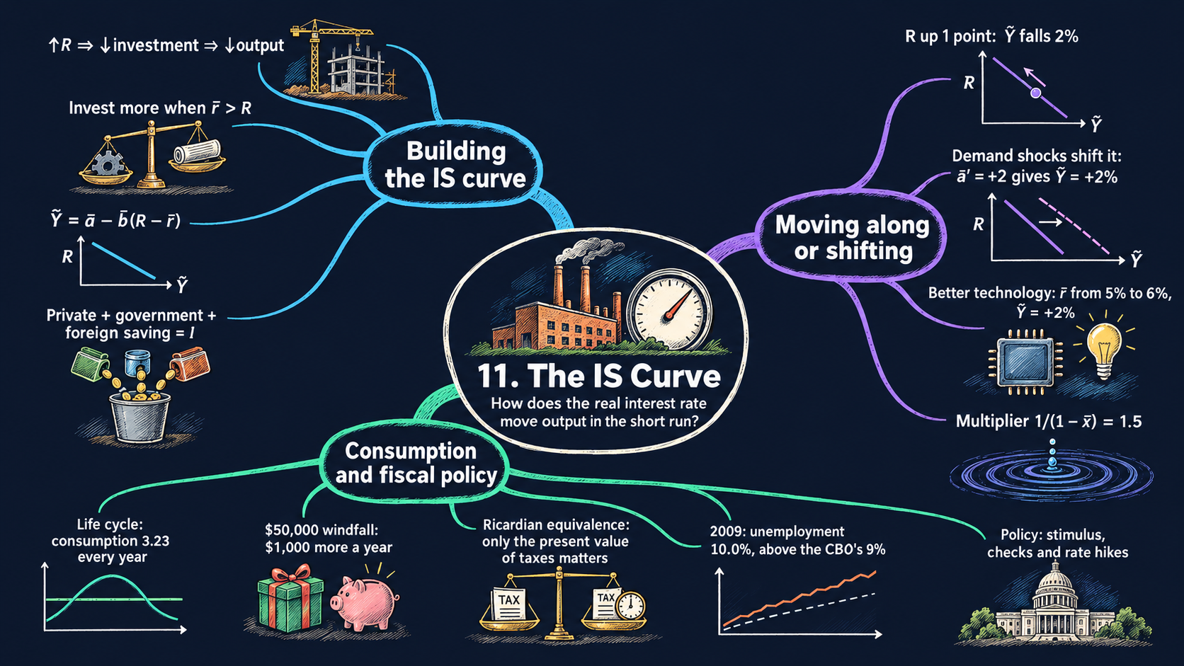
Chapter 9 measured the ups and downs of the economy. This chapter builds the first piece of the model that explains them: the IS curve, which links the real interest rate to short-run output. By the end of it you will be able to:
- derive the IS curve \(\tilde{Y}_t = \bar{a} - \bar{b}(R_t - \bar{r})\) step by step from the national income identity and the five demand equations, and explain why it slopes down and why “IS” means investment equals saving;
- read the comparative statics of the IS curve: tell a movement along it (a change in the real interest rate) from a shift (an aggregate demand shock or a change in the marginal product of capital), and say by how much output changes;
- derive the multiplier \(1/(1-\bar{x})\) in two ways, by solving the model and by adding up the rounds of spending;
- explain the life-cycle / permanent-income theory of consumption, compute permanent income as a present value, and explain why only the present value of taxes matters (Ricardian equivalence);
- compare the Congressional Budget Office’s 2009 forecasts of unemployment with what actually happened;
- in Python: reuse one model function in many figures, shade areas between two curves, and summarize monthly data by quarter and year with
groupby.
Model overview
Back on Islandia, the island country whose tools we counted in Chapter 5, Harbor Boatworks is thinking about a new boat shed. The firm would pay for it with a loan, so it compares two numbers: what the shed would earn each year, and the interest on the loan. This year the Bank of Islandia has pushed the real interest rate up, fewer sheds pay for themselves, and Islandia spends less on new tools. How far below its potential level does Islandia’s output then fall? This section answers with the IS curve, the first building block of the short-run model, and follows Islandia through every step.
NoteThe big idea
The question. When the real interest rate rises, how far does output fall below its potential level, and why?
The answer in one sentence. A real interest rate above the return on new capital cuts investment, and with less spending, output falls below potential; the downward-sloping line that links the interest rate to short-run output is the IS curve.
What goes in and what comes out. We choose the normal share of each kind of spending, how strongly investment reacts to the interest rate, the marginal product of capital and, for now, the real interest rate itself. The model gives back short-run output, the percentage gap between actual and potential output, together with every use of output. The second block adds the size of the multiplier, and the third gives the spending plan of a household that smooths its consumption over a lifetime.
Road map.
- The IS curve: the assumptions, solving the model step by step, and what the model predicts: moving along the curve versus shifting it.
- The multiplier: what changes when islanders’ consumption reacts to booms and slumps.
- Permanent income and consumption smoothing: the household decision behind the consumption equation, and why the timing of taxes may not matter.
- Model in code: the Key results as Python functions, checked with numbers, plus the drawing tools that every figure reuses.
Notation. As everywhere in the book, a bar over a letter marks something the short-run model takes as given: a parameter such as \(\bar{b}\), or a value handed over by the long-run model, such as potential output \(\bar{Y}_t\) and the marginal product of capital \(\bar{r}\). Letters without a bar are endogenous variables. The real interest rate \(R_t\) has no bar because Chapter 12 will make it endogenous; in this chapter we simply take it as given. In the code we write a, b and r_bar.
| Symbol | Meaning | Type |
|---|---|---|
| \(Y_t\) | output (GDP) in period \(t\) | endogenous |
| \(C_t, I_t, G_t\) | consumption, investment and government purchases | endogenous |
| \(EX_t, IM_t\) | exports to and imports from the rest of the world | endogenous |
| \(\tilde{Y}_t\) | short-run output: the percentage gap between \(Y_t\) and \(\bar{Y}_t\) | endogenous |
| \(\bar{Y}_t\) | potential output, from the long-run model | parameter |
| \(R_t\) | the real interest rate: given in this chapter, endogenous from Chapter 12 | parameter |
| \(\bar{r}\) | the marginal product of capital: what a new unit of capital earns | parameter |
| \(\bar{a}_c, \bar{a}_i, \bar{a}_g, \bar{a}_{ex}, \bar{a}_{im}\) | the normal shares of each use of output in potential output | parameters |
| \(\bar{a}\) | the aggregate demand shock, built from the five shares | parameter |
| \(\bar{b}\) | how strongly investment reacts to the interest rate | parameter |
| \(\bar{x}\) | how strongly consumption reacts to short-run output (second block) | parameter |
| \(T_t\) | tax revenue (step 7 only) | parameter |
| \(y_t, y^p\) | a household’s income in period \(t\), and its permanent income (third block) | parameter, endogenous |
| \(\Delta x\) | the change in \(x\) | notation |
The IS curve
Assumptions
Time runs in periods \(t\) (think of quarters or years). Six equations describe Islandia’s short run, and each of them holds in every period.
1. Where output goes. Everything Islandia produces ends up in one of four places. Islanders consume it, Harbor Boatworks invests it in new tools, the Islandia Treasury buys it, or Mainland buys it as exports. Goods that Islandia buys from Mainland are subtracted, because they were made abroad (Chapter 2):
\[Y_t = C_t + I_t + G_t + EX_t - IM_t. \tag{1}\]
This is the national income identity. Add \(IM_t\) to both sides and it reads the other way round: what Islandia produces plus what it brings in from Mainland is everything it has to work with, and it uses all of it in exactly four ways.
2 to 5. Four uses of output that track potential output. Consumption, government purchases, exports and imports are each a fixed share of potential output:
\[C_t = \bar{a}_c\bar{Y}_t, \qquad G_t = \bar{a}_g\bar{Y}_t, \qquad EX_t = \bar{a}_{ex}\bar{Y}_t, \qquad IM_t = \bar{a}_{im}\bar{Y}_t.\]
Potential output \(\bar{Y}_t\) is what Islandia would make with all its workers and tools fully employed. The long-run model of Chapters 5 and 6 pins it down, so here it is given. Tying consumption to \(\bar{Y}_t\), and not to actual output \(Y_t\), is a real assumption about behavior:
- potential output moves slowly, so when a slump pulls \(Y_t\) down, \(\bar{Y}_t\) barely changes;
- so islanders keep spending much as before, for instance by drawing on their savings.
The third block explains why households behave this way. As rough benchmarks for the United States, consumption is close to two thirds of GDP and government purchases close to one fifth.
6. Investment reacts to the interest rate. The investment share has a normal level \(\bar{a}_i\). It rises above that level or falls below it depending on how the real interest rate \(R_t\) compares with the marginal product of capital \(\bar{r}\):
\[\frac{I_t}{\bar{Y}_t} = \bar{a}_i - \bar{b}\,(R_t - \bar{r}). \tag{2}\]
Why does the gap matter? Take one unit of output that Harbor Boatworks could turn into a new tool. Installed, the tool yields \(\bar{r}\) extra units of output a period later. Put in the bank instead, or used to pay off a loan, the same unit earns \(R_t\). Say \(\bar{r} = 5\) percent and \(R_t = 3\) percent. If the firm borrows 100 units and builds a shed with them, the shed adds 5 units of output, the loan costs 3 units of interest, and 2 units are left over. Projects like this pay, so investment rises above normal. When \(R_t\) is above \(\bar{r}\), the bank wins, and the firm builds less than usual. The parameter \(\bar{b} > 0\) measures how strongly firms respond: each percentage point of gap moves investment by \(\bar{b}\) percentage points of potential output.
In the long run the two rates are equal, \(R_t = \bar{r}\). Firms keep adding capital until its marginal product falls to the interest rate, as in the Solow model of Chapter 5, and investment rests at its normal share \(\bar{a}_i\). In the short run the two rates can differ. The Bank of Islandia can move \(R_t\) within a day, while the marginal product of capital changes only as new sheds and boats are built and put to work. \(\bar{r}\) has no time subscript because it is constant along a balanced growth path; \(\bar{Y}_t\) keeps its subscript because potential output grows.
Here is the whole model: six equations for six endogenous variables, \(Y_t\), \(C_t\), \(I_t\), \(G_t\), \(EX_t\) and \(IM_t\).
| Equation | Name | What it takes as given |
|---|---|---|
| \(Y_t = C_t + I_t + G_t + EX_t - IM_t\) | national income identity | nothing |
| \(C_t = \bar{a}_c\bar{Y}_t\) | consumption | \(\bar{a}_c\), \(\bar{Y}_t\) |
| \(G_t = \bar{a}_g\bar{Y}_t\) | government purchases | \(\bar{a}_g\), \(\bar{Y}_t\) |
| \(EX_t = \bar{a}_{ex}\bar{Y}_t\) | exports | \(\bar{a}_{ex}\), \(\bar{Y}_t\) |
| \(IM_t = \bar{a}_{im}\bar{Y}_t\) | imports | \(\bar{a}_{im}\), \(\bar{Y}_t\) |
| \(I_t/\bar{Y}_t = \bar{a}_i - \bar{b}(R_t - \bar{r})\) | investment | \(\bar{a}_i\), \(\bar{b}\), \(\bar{r}\), \(\bar{Y}_t\), and for now \(R_t\) |
Islandia’s baseline: the numbers used in this notebook. Every IS diagram starts from one set of values, the ones the textbook uses in its own diagrams: no aggregate demand shock, \(\bar{a} = 0\); a sensitivity of investment \(\bar{b} = 2\); and a marginal product of capital \(\bar{r} = 5\) percent. For the demand shares we pick illustrative values, in percent of potential output, that add up to 100: consumption \(\bar{a}_c = 65\), investment \(\bar{a}_i = 17\), government purchases \(\bar{a}_g = 20\), exports \(\bar{a}_{ex} = 12\) and imports \(\bar{a}_{im} = 14\). We measure \(\tilde{Y}\), \(R\), \(\bar{r}\) and \(\bar{a}\) in percent (or percentage points), so every number below is a percentage.
Harbor Boatworks invests more when a new tool earns more than a loan costs, and less when it earns less.
NoteCheck your understanding
1. In the baseline, \(\bar{a}_i = 17\), \(\bar{b} = 2\) and \(\bar{r} = 5\) percent. The Bank of Islandia lowers the real interest rate to 3 percent. What share of potential output does Harbor Boatworks now invest?
Answer
By equation (2), \(I_t/\bar{Y}_t = 17 - 2\times(3 - 5) = 17 + 4 = 21\) percent of potential output: 4 points above normal, because each new tool now earns 2 points more than the loan costs.
2. The Bank raises the real interest rate to 8 percent. At the same time, a new hull design raises the marginal product of capital to 8 percent too. Does investment change?
Answer
No. Equation (2) depends only on the gap \(R_t - \bar{r}\), which is still zero, so investment stays at its normal share, \(\bar{a}_i = 17\) percent of potential output. A high interest rate does not hold investment back when new tools earn just as much.
Solving the model
Step 1: write every use of output as a share of potential output. Divide both sides of the identity (1) by \(\bar{Y}_t\). Each term becomes a share:
\[\frac{Y_t}{\bar{Y}_t} = \frac{C_t}{\bar{Y}_t} + \frac{I_t}{\bar{Y}_t} + \frac{G_t}{\bar{Y}_t} + \frac{EX_t}{\bar{Y}_t} - \frac{IM_t}{\bar{Y}_t}.\]
Step 2: substitute the demand equations. Divide each of assumptions 2 to 5 by \(\bar{Y}_t\): \(C_t/\bar{Y}_t = \bar{a}_c\), \(G_t/\bar{Y}_t = \bar{a}_g\), \(EX_t/\bar{Y}_t = \bar{a}_{ex}\) and \(IM_t/\bar{Y}_t = \bar{a}_{im}\). Equation (2) already gives the investment share. Put all five on the right-hand side:
\[\frac{Y_t}{\bar{Y}_t} = \bar{a}_c + \big[\bar{a}_i - \bar{b}\,(R_t - \bar{r})\big] + \bar{a}_g + \bar{a}_{ex} - \bar{a}_{im}.\]
Five of the six unknowns are gone. Only \(Y_t\) is left, and it depends on the interest rate and on parameters.
Step 3: from the output ratio to short-run output. Short-run output, defined in Chapter 9, is the percentage gap between actual and potential output. Split the fraction in two to see how it relates to the ratio on the left of step 2:
\[\tilde{Y}_t \equiv \frac{Y_t - \bar{Y}_t}{\bar{Y}_t} = \frac{Y_t}{\bar{Y}_t} - \frac{\bar{Y}_t}{\bar{Y}_t} = \frac{Y_t}{\bar{Y}_t} - 1.\]
For small gaps, \(\tilde{Y}_t \approx \ln Y_t - \ln\bar{Y}_t\) (Appendix C.6). So \(\tilde{Y}_t = -0.02\), or \(-2\) percent, means that Islandia produces 2 percent less than its potential.
Step 4: subtract 1 from both sides. The left side of step 2 becomes \(\tilde{Y}_t\). On the right, gather the constant terms into one group:
\[\tilde{Y}_t = \underbrace{\bar{a}_c + \bar{a}_i + \bar{a}_g + \bar{a}_{ex} - \bar{a}_{im} - 1}_{\text{call it } \bar{a}} - \bar{b}\,(R_t - \bar{r}).\]
Give the group a name, \(\bar{a}\), and six equations have shrunk to one straight line:
ImportantKey result: the IS curve
\[\tilde{Y}_t = \bar{a} - \bar{b}\,(R_t - \bar{r}), \qquad \bar{a} \equiv \bar{a}_c + \bar{a}_i + \bar{a}_g + \bar{a}_{ex} - \bar{a}_{im} - 1. \tag{3}\]
Short-run output falls as the real interest rate rises above the marginal product of capital, by \(\bar{b}\) points for each point of gap. The aggregate demand shock \(\bar{a}\) sets where the line sits.
Islandia in numbers. In the baseline, \(\bar{a} = 0\), \(\bar{b} = 2\) and \(\bar{r} = 5\) percent. A real interest rate of 4 percent gives \(\tilde{Y} = 0 - 2\times(4 - 5) = +2\) percent, and one of 7 percent gives \(\tilde{Y} = 0 - 2\times(7 - 5) = -4\) percent.
TipIn words
Islandia’s output can leave its potential for two reasons. The first is \(\bar{a}\), the aggregate demand shock: it packs the five spending shares into one number, which says how far total spending at normal interest rates sits from potential output. The second is the interest-rate term, and there only the gap \(R_t - \bar{r}\) counts, not the level of \(R_t\). A high interest rate does not stop Harbor Boatworks from building if each new shed earns just as much.
Step 5: the long-run value of \(\bar{a}\). In the long run Islandia produces at potential, \(\tilde{Y}_t = 0\), and the interest rate equals the marginal product of capital, \(R_t = \bar{r}\). Put both into equation (3): \(0 = \bar{a} - \bar{b}\times 0\), so \(\bar{a} = 0\). Through the definition of \(\bar{a}\), this means that at potential the five spending shares add up to exactly one: \(\bar{a}_c + \bar{a}_i + \bar{a}_g + \bar{a}_{ex} - \bar{a}_{im} = 1\). Islandia’s baseline shares pass this test, since \(65 + 17 + 20 + 12 - 14 = 100\) percent. So \(\bar{a} = 0\) is the normal case, and shocks to spending push \(\bar{a}\) away from zero for a while.
Step 6: the curve on a graph. The textbook draws the curve with output across and the interest rate up, so we solve equation (3) for \(R_t\). Move the interest-rate term to the left and \(\tilde{Y}_t\) to the right, then divide by \(\bar{b}\) (Appendix C.9):
\[\bar{b}\,(R_t - \bar{r}) = \bar{a} - \tilde{Y}_t \quad\Longrightarrow\quad R_t = \bar{r} + \frac{\bar{a} - \tilde{Y}_t}{\bar{b}}.\]
In this form the IS curve is a line with slope \(-1/\bar{b}\) through the point \((\tilde{Y}, R) = (\bar{a}, \bar{r})\). With \(\bar{b} = 2\) the slope is \(-0.5\): to raise output by one point, the interest rate must fall by half a point. A larger \(\bar{b}\) gives a flatter line.
The same numbers, share by share. The Key result gave Islandia’s output at two interest rates in one step. Building it up from the six equations gives the same answers:
- at \(R = 4\) percent, investment is \(17 - 2\times(4 - 5) = 19\) percent of potential output, so \(Y/\bar{Y} = 65 + 19 + 20 + 12 - 14 = 102\) percent and \(\tilde{Y} = +2\) percent;
- at \(R = 7\) percent, investment is \(17 - 2\times 2 = 13\) percent, \(Y/\bar{Y} = 96\) percent and \(\tilde{Y} = -4\) percent.
Step 7: why the curve is called “IS”. The letters stand for investment equals saving, and the identity (1) shows why. Keep investment on the right and move every other term to the left:
\[Y_t - C_t - G_t + (IM_t - EX_t) = I_t.\]
Now add and subtract tax revenue \(T_t\) on the left. Since \(-T_t + T_t = 0\), only the grouping changes:
ImportantKey result: investment equals saving
\[\underbrace{(Y_t - T_t - C_t)}_{\text{private saving}} + \underbrace{(T_t - G_t)}_{\text{government saving}} + \underbrace{(IM_t - EX_t)}_{\text{foreign saving}} = I_t. \tag{4}\]
Three kinds of saving together pay for investment: what islanders keep from their after-tax income, the Treasury’s surplus, and what Mainland lends Islandia when it ships more goods than it buys.
Islandia in numbers. At potential, with the baseline shares and taxes of, say, 18 percent of potential output, private saving is \(100 - 18 - 65 = 17\), government saving is \(18 - 20 = -2\) (a deficit) and foreign saving is \(14 - 12 = 2\). Total saving is 17 percent of potential output, exactly the investment share.
Each piece has a plain meaning. Households save the part of their after-tax income that they do not consume. The Islandia Treasury saves when its tax revenue exceeds its purchases, that is, when it runs a surplus. Mainland saves in Islandia when it ships Islandia more goods than it buys from it, because it is lending Islandia the difference. John Hicks introduced the curve in 1937, as a compact algebraic version of Keynes’s General Theory. Equation (4) returns when the book studies budget deficits and the trade balance.
Six equations shrink to one downward-sloping line: an interest rate above the return on capital means output below potential.
NoteCheck your understanding
1. In the baseline, the Bank of Islandia sets the real interest rate at 6 percent. What share of potential output is invested, and what is short-run output?
Answer
By equation (2), investment is \(17 - 2\times(6 - 5) = 15\) percent of potential output. Adding up the uses, \(Y/\bar{Y} = 65 + 15 + 20 + 12 - 14 = 98\) percent, so output is 2 percent below potential. Equation (3) gives the same answer in one step: \(\tilde{Y} = 0 - 2\times(6 - 5) = -2\).
2. At potential, with \(R = \bar{r}\), the Islandia Treasury raises taxes from 18 to 20 percent of potential output and keeps its purchases unchanged. Which kinds of saving in equation (4) change, and does total saving still equal investment?
Answer
In this block consumption follows potential output, so it stays at its share of 65. Private saving falls to \(100 - 20 - 65 = 15\) percent, government saving rises to \(20 - 20 = 0\), and foreign saving stays at \(14 - 12 = 2\) percent. Total saving is still 17 percent, the investment share: equation (4) is an identity, so it holds whatever the Treasury does.
What the model predicts
Comparative statics. Equation (3) is linear, so each effect is a constant: the derivative of \(\tilde{Y}_t\) with respect to that parameter (Appendix C.7). Because \(\tilde{Y}\) is already a percentage, each number reads as “percent of potential output per percentage point”.
| A rise of 1 point in … | changes \(\tilde{Y}_t\) (at a given \(R_t\)) by | baseline value | What happens to the IS curve |
|---|---|---|---|
| the real interest rate \(R_t\) | \(-\bar{b}\) | \(-2\) | nothing: the economy moves up along the curve |
| \(\bar{a}_c\), \(\bar{a}_i\), \(\bar{a}_g\) or \(\bar{a}_{ex}\) (so \(\bar{a}\)) | \(+1\) | \(+1\) | shifts right by 1 point |
| imports \(\bar{a}_{im}\) | \(-1\) | \(-1\) | shifts left by 1 point |
| the marginal product of capital \(\bar{r}\) | \(+\bar{b}\) | \(+2\) | shifts up by 1 point (right by \(\bar{b}\) points) |
| the sensitivity \(\bar{b}\) | \(-(R_t - \bar{r})\) | \(0\) at \(R_t = \bar{r}\) | rotates around the point \((\bar{a}, \bar{r})\) and gets flatter |
| potential output \(\bar{Y}_t\) | \(0\) | \(0\) | nothing: \(\bar{Y}_t\) is not in equation (3) |
What the signs mean for Islandia:
- Along or shift. The IS curve plots output against the interest rate, so a change in \(R_t\) is read off the curve itself: a movement along it. A change in anything else in equation (3) changes the output that goes with each interest rate: a shift of the whole curve.
- Demand shocks pass into output one for one. Suppose Harbor Boatworks grows optimistic about a new boat design and raises \(\bar{a}_i\) by 1 point. Then \(\bar{a}\) goes from 0 to 1 and, at an unchanged interest rate, output ends up 1 percent above potential. It works the same way in reverse for gloomy islanders (\(\bar{a}_c\) falls), cuts in Treasury purchases (\(\bar{a}_g\) falls) or a slump on Mainland that lowers the demand for Islandia’s exports (\(\bar{a}_{ex}\) falls). The last case is how recessions travel from one country to another.
- The slope comes from investment. The more strongly investment reacts to the interest rate (a larger \(\bar{b}\)), the more output moves when the interest rate moves.
- Potential output does not shift the curve. When a new technology lifts potential output, actual output rises in the same proportion, so the gap \(\tilde{Y}_t\) stays the same. A storm that wrecks part of Islandia’s tools works the same way: actual and potential output fall together.
- But the return on capital does. The same technology, or the same storm, can also raise the marginal product of capital \(\bar{r}\): the tools that survive, or the tools that use the new ideas, earn more. At an unchanged \(R_t\) investment rises, and output goes up by \(\bar{b}\) points for every point of \(\bar{r}\).
A change in the interest rate moves Islandia along its IS curve; a change in anything else shifts the whole curve.
NoteCheck your understanding
1. A slump on Mainland cuts Islandia’s export share from 12 to 10 percent of potential output, and the Bank keeps the real interest rate at \(\bar{r} = 5\) percent. What is the new \(\bar{a}\), where is output, and how does the IS curve move?
Answer
By the definition in equation (3), \(\bar{a} = 65 + 17 + 20 + 10 - 14 - 100 = -2\). At \(R = \bar{r}\), output is 2 percent below potential. The whole curve shifts left by 2 points, the same kind of shift as for the pessimistic consumers of Fig. 8.
2. A better hull design raises the marginal product of capital from 5 to 6 percent, while the Bank keeps the real interest rate at 5 percent. Why does output rise, and by how much?
Answer
A new tool now earns 1 point more than a loan costs, so Harbor Boatworks builds more. By equation (3), \(\tilde{Y} = 0 - 2\times(5 - 6) = +2\) percent: \(\bar{b}\) points of output for each point of \(\bar{r}\). The IS curve shifts up by 1 point, as in Fig. 9.
The multiplier
Assumptions
Keep every assumption of the IS curve except the consumption equation. Consumption now also reacts to booms and slumps:
\[\frac{C_t}{\bar{Y}_t} = \bar{a}_c + \bar{x}\,\tilde{Y}_t, \qquad 0 < \bar{x} < 1.\]
When Islandia’s output is 1 percent above potential, islanders consume \(\bar{x}\) percent of potential output more than their normal share. The parameter \(\bar{x}\) stands for households that spend part of a short-lived rise in income instead of smoothing it away. The third block shows why such households show up in the data.
Solving the model
Step 1: redo the derivation with the new consumption share. Steps 1 to 4 of the IS curve go through as before, with one extra term on the right, because \(C_t/\bar{Y}_t\) now equals \(\bar{a}_c + \bar{x}\tilde{Y}_t\):
\[\tilde{Y}_t = \bar{a} + \bar{x}\,\tilde{Y}_t - \bar{b}\,(R_t - \bar{r}),\]
with \(\bar{a}\) defined exactly as in equation (3). Short-run output now appears on both sides.
Step 2: solve for \(\tilde{Y}_t\). Subtract \(\bar{x}\tilde{Y}_t\) from both sides, factor out \(\tilde{Y}_t\), and divide by \(1 - \bar{x}\), which is positive because \(\bar{x} < 1\):
\[\tilde{Y}_t - \bar{x}\,\tilde{Y}_t = \bar{a} - \bar{b}\,(R_t - \bar{r}) \quad\Longrightarrow\quad (1 - \bar{x})\,\tilde{Y}_t = \bar{a} - \bar{b}\,(R_t - \bar{r}).\]
ImportantKey result: the IS curve with a multiplier
\[\tilde{Y}_t = \frac{1}{1 - \bar{x}}\times\big[\bar{a} - \bar{b}\,(R_t - \bar{r})\big] \tag{5}\]
The factor \(1/(1 - \bar{x})\) is the multiplier. Since \(\bar{x}\) lies between 0 and 1, it is larger than 1: every effect of equation (3) is scaled up.
Islandia in numbers. With \(\bar{x} = 1/3\) the multiplier is \(1/(2/3) = 1.5\), and with \(\bar{x} = 1/2\) it is 2. In the baseline with \(\bar{x} = 1/3\), a 1-point rise in the interest rate lowers output by \(2\times 1.5 = 3\) percent instead of 2 percent.
Step 3: the same result, round by round. Where does the extra output come from? Let the interest rate rise by 1 point in the baseline. Investment falls by \(\bar{b} = 2\) points of potential output, so in the first round output falls by 2 percent. Lower output means lower incomes, and consumption falls by \(\bar{x}\) times that, \(\frac{1}{3}\times 2 = \frac{2}{3}\) of a point: a second round. That cut in spending lowers other incomes and trims consumption again, by \(\frac{1}{3}\times\frac{2}{3} = \frac{2}{9}\) of a point, and so on. Adding up all the rounds:
\[\Delta\tilde{Y} = -2\,\big(1 + \bar{x} + \bar{x}^2 + \bar{x}^3 + \cdots\big).\]
The bracket is a geometric series (Appendix C.12). Call it \(S\). Multiplying by \(\bar{x}\) moves every term one place along, \(\bar{x}S = \bar{x} + \bar{x}^2 + \bar{x}^3 + \cdots\), and subtracting this from \(S\) leaves only the first term: \(S - \bar{x}S = 1\), so \(S = 1/(1 - \bar{x})\). The total is \(-2\times 1.5 = -3\) percent, exactly what equation (5) gives. The series adds up to a finite number only when \(\bar{x} < 1\), which is why the model needs that assumption: if every lost unit of income cut spending by a unit or more, the rounds would never die out.
TipIn words: the rounds of spending
Harbor Boatworks builds fewer sheds, so its boatbuilders earn less. They spend less at the island’s market, so the stallholders earn less, and they in turn spend a little less too. Each round is a third the size of the one before, so the echoes fade, but together they make the first fall half as large again.
Step 4: a second route to a multiplier, through investment. Multiply equation (2) by \(\bar{Y}_t\) to write investment in levels:
\[I_t = \bar{a}_i\bar{Y}_t - \bar{b}\,(R_t - \bar{r})\,\bar{Y}_t.\]
Investment grows in step with potential output. One reason is cash flow, the funds firms have left after paying their costs. Harbor Boatworks can pay for a shed more cheaply out of its own funds than with a loan, and the cash flow of all firms together moves roughly with potential output. If cash flow also rises in a boom, investment gets an extra term in \(\tilde{Y}_t\). Write it, with a label of our own, as \(+\bar{z}\tilde{Y}_t\) in the investment share. Then steps 1 and 2 give a multiplier of \(1/(1 - \bar{x} - \bar{z})\), as long as \(\bar{x} + \bar{z} < 1\). The curve keeps the same form; only the size of the multiplier changes.
What the model predicts
Comparative statics with and without the multiplier. Differentiate equation (5) and compare with equation (3):
| Effect | IS curve (3) | with the multiplier (5) | baseline, \(\bar{x} = 1/3\) |
|---|---|---|---|
| a 1-point demand shock \(\bar{a}\) | \(+1\) | \(+1/(1-\bar{x})\) | \(+1\) → \(+1.5\) |
| a 1-point rise in \(R_t\) | \(-\bar{b}\) | \(-\bar{b}/(1-\bar{x})\) | \(-2\) → \(-3\) |
| a 1-point rise in \(\bar{r}\) | \(+\bar{b}\) | \(+\bar{b}/(1-\bar{x})\) | \(+2\) → \(+3\) |
| slope of the curve in the diagram, \(dR/d\tilde{Y}\) | \(-1/\bar{b}\) | \(-(1-\bar{x})/\bar{b}\) | \(-0.5\) → \(-0.33\) (flatter) |
- Every shock is amplified. Spending feeds on itself: a fall in one kind of demand lowers incomes, which lowers consumption, which lowers incomes again. The same chain enlarges good news, so the IS curve can produce “vicious” and “virtuous” circles.
- The form of the curve does not change. Define \(\bar{a}^m \equiv \bar{a}/(1-\bar{x})\) and \(\bar{b}^m \equiv \bar{b}/(1-\bar{x})\). Then equation (5) reads \(\tilde{Y}_t = \bar{a}^m - \bar{b}^m(R_t - \bar{r})\): equation (3) with larger coefficients. That is why the rest of the book keeps writing equation (3) and lets \(\bar{a}\) and \(\bar{b}\) include any multiplier.
- Fiscal policy is stronger, unless something offsets it. If the Islandia Treasury raises its purchases by 1 point of potential output, \(\bar{a}_g\) rises, and output rises by \(1/(1-\bar{x})\) points at a given interest rate. The next block shows why the way the spending is paid for can offset part of this.
When islanders spend part of every change in income, each shock echoes through the economy and grows by the multiplier.
NoteCheck your understanding
1. Suppose islanders spend half of every change in short-run output, \(\bar{x} = 1/2\). The Treasury raises its purchases by 1 point of potential output, and the interest rate does not move. By how much does output rise?
Answer
The multiplier is \(1/(1 - 1/2) = 2\). The shock raises \(\bar{a}\) by 1 point, so by equation (5) output rises by 2 percent of potential: 1 point from the Treasury’s own purchases and 1 more from the rounds of extra consumption.
2. Why does the model need \(\bar{x} < 1\)? What would go wrong if every unit of lost income cut spending by a full unit?
Answer
With \(\bar{x} = 1\) each round of the geometric series in step 3 would be as large as the one before, so the sum \(1 + 1 + 1 + \cdots\) would never stop growing, and \(1/(1 - \bar{x})\) in equation (5) would mean dividing by zero. A shock would never die out.
Permanent income and consumption smoothing
Assumptions
This block looks behind the consumption equation \(C_t = \bar{a}_c\bar{Y}_t\) at the decision of the islanders it stands for.
- Islanders prefer a smooth path of consumption. Marginal utility diminishes: each extra unit of consumption in a period adds less satisfaction than the one before. So a steady amount every period beats plenty in some periods and little in others, even when the total is the same.
- Islanders can borrow and lend at a constant real interest rate \(R\), here written as a decimal.
- The budget holds over a whole life. Over a life of \(T\) periods, the present discounted value of consumption equals the present discounted value of income (Appendix C.12; present values first appear in Chapter 7). Borrowing and saving can move consumption between periods, but cannot raise its total value.
Solving the model
Step 1: define permanent income. An islander’s income stream is \(y_0, y_1, \dots, y_{T-1}\). Their permanent income \(y^p\) is the constant amount per period whose stream is worth the same in present value:
\[\sum_{t=0}^{T-1}\frac{y^p}{(1+R)^t} = \sum_{t=0}^{T-1}\frac{y_t}{(1+R)^t}.\]
Step 2: solve for \(y^p\). \(y^p\) is the same in every term on the left, so it factors out of the sum. Dividing both sides by the sum that is left gives \(y^p\) as a ratio of two present values.
ImportantKey result: permanent income
\[\sum_{t=0}^{T-1}\frac{y^p}{(1+R)^t} = \sum_{t=0}^{T-1}\frac{y_t}{(1+R)^t} \tag{6}\]
\[y^p = \frac{\sum_{t=0}^{T-1} y_t/(1+R)^t}{\sum_{t=0}^{T-1} 1/(1+R)^t}\]
Permanent income is a weighted average of income, with weights that shrink the further a period lies in the future. A household that wants smooth consumption sets \(c_t = y^p\) in every period. By equation (6) this plan costs exactly what the household earns, in present value, so it meets the lifetime budget.
TipIn words
An islander looks at the whole path of income ahead, from the lean school years through the busy years at the boatworks to retirement, and turns it into one steady number. That number, not this year’s pay, decides how much the islander spends each year. Lean years are covered by borrowing or by savings, and fat years are partly saved.
Step 3: no interest, the life-cycle model. With \(R = 0\) every weight equals 1 and the denominator is just \(T\), so \(y^p = \frac{1}{T}\sum_t y_t\): consumption equals average lifetime income. That is the life-cycle model of Fig. 5. Young islanders consume more than they earn, middle-aged workers save, and retirees live on what they saved.
Step 4: a windfall. Suppose an islander who plans to live forever receives an unexpected gift \(W\) today. If the gift stays in the bank and the islander consumes only the interest it earns, they can spend \(\Delta c = R\,W\) more in every future period without ever touching the gift. The present value of that extra spending, starting next period, is a geometric series with ratio \(q = 1/(1+R)\):
\[\sum_{t=1}^{\infty}\frac{R\,W}{(1+R)^t} = R\,W\,\frac{q}{1-q} = R\,W\times\frac{1/(1+R)}{R/(1+R)} = R\,W\times\frac{1}{R} = W.\]
So the permanent rise in consumption is the interest on the windfall. With \(R = 2\) percent, a gift of 50,000 raises consumption by 1,000 a year, not by 50,000 this year.
Step 5: the timing of taxes. Suppose the Islandia Treasury needs a tax of \(\tau\) from you. It can collect \(\tau\) today, or borrow, spend now, and collect \((1+R)\tau\) next period to repay the loan with interest. In present value the two are the same, \((1+R)\tau/(1+R) = \tau\), so they lower your permanent income, and your consumption, by the same amount. The idea that only the present value of taxes matters for consumption, not their timing, is called Ricardian equivalence.
What the model predicts
- Consumption is smoother than income. It follows permanent income, which changes little when income moves for a short time. This justifies \(C_t = \bar{a}_c\bar{Y}_t\) in the IS curve: in a slump that islanders expect to be short, \(Y_t\) falls but permanent income barely moves, so consumption holds up. A strict version of the theory would smooth even the predictable growth of potential output, so our equation captures the idea only in part.
- Large, predictable changes in income are smoothed; small surprises are partly spent. Studies of individual households support the first part well and the second part less well. Spending out of temporary income is what the parameter \(\bar{x}\) of the multiplier block captures.
- How spending is paid for matters for fiscal policy. Extra government purchases raise \(\bar{a}_g\). If islanders expect higher taxes to pay for them, now or later, their permanent income falls and \(\bar{a}_c\) falls too, which offsets part of the shift of the IS curve. If the extra spending today is simply spending moved forward from the future, there is no extra tax burden, consumption does not fall, and the IS curve shifts out by the full amount. Chapter 16 studies consumption, and Chapter 18 the government budget, in more depth.
Islanders spend according to their lifetime income, so short-lived ups and downs in income barely move their consumption.
NoteCheck your understanding
1. The real interest rate is 4 percent, and an islander who plans to live forever wins a prize of 20,000. How much more can the islander consume every year, for good?
Answer
By step 4, the permanent rise in consumption is the interest on the prize: \(\Delta c = R\,W = 0.04\times 20{,}000 = 800\) a year. Its present value is exactly the prize, so the plan fits the lifetime budget of equation (6).
2. The Treasury cuts an islander’s tax by 1,000 today and pays for the cut by borrowing. Next year it raises the same islander’s tax by 1,020, with \(R = 2\) percent. Does the islander consume more today?
Answer
No. In present value the later tax is \(1{,}020/1.02 = 1{,}000\), exactly the cut, so permanent income in equation (6) does not change, and neither does consumption. The islander simply saves the tax cut to pay next year’s tax. This is Ricardian equivalence (step 5).
NoteRecap
- One line links the interest rate to output: the IS curve \(\tilde{Y}_t = \bar{a} - \bar{b}(R_t - \bar{r})\) follows from the national income identity and five demand equations (Fig. 2).
- Investment is the channel: when the real interest rate rises above the marginal product of capital, firms invest less and output falls below potential (Fig. 1).
- Along or shift: a change in \(R_t\) moves the economy along the curve (Fig. 7); a demand shock or a new \(\bar{r}\) shifts it (Fig. 4, Fig. 9).
- IS means investment equals saving: private, government and foreign saving together finance investment, equation (4).
- The multiplier \(1/(1-\bar{x})\) amplifies every shock when consumption reacts to short-run output, but leaves the form of the curve unchanged.
- Consumption follows permanent income: people smooth spending over their lives, and only the present value of taxes matters for it (Fig. 5).
Model in code
Now we turn the Key results into Python. The section has four parts: the setup (folded, because it is the same in every chapter), the model as functions, numerical checks of the Key results with Islandia’s numbers, and the drawing tools that every IS diagram uses (folded too). Run its cells once, in order. Every later section of the notebook reuses them.
Setup
Run the setup cells once, before anything else. They load the Python libraries, give every chart the same look, store the address of the chapter’s data and define one helper that only the book website needs. You can use the notebook without reading them; open the box if you are curious.
NoteShow the setup code
The first cell loads the libraries and sets the look of the charts. Its comments explain each step.
The website cannot run Python, so each interactive figure also gets a version with a precomputed slider. The next helper builds those versions. Run it and move on.
# @title Helper for the website versions (run this cell; you do not need to read it)
def slider_figure(make_figure, name, values, start, label=None):
    """Join precomputed versions of a figure with one slider (the website cannot run Python).

    Arguments
        make_figure : the function that draws the figure, e.g. is_diagram
        name        : the argument the slider moves, e.g. "b"
        values      : the values of that argument to precompute
        start       : the value shown first
        label       : the slider's label (the argument name if None)
    Returns
        one Plotly figure with all versions and a slider that shows one at a time
    """
    # Step 1: draw the figure once for every value
    figures = [make_figure(**{name: v}) for v in values]
    first = values.index(start)
    # Step 2: copy every curve into one figure; only the start value's are visible
    fig = go.Figure(layout=figures[first].layout)
    owner = []                          # which precomputed figure each trace is from
    for i, f in enumerate(figures):
        for trace in f.data:
            trace.visible = (i == first)
            fig.add_trace(trace)
            owner.append(i)
    # Step 3: one slider step per value: its curves, title, labels and shapes
    steps = []
    for i, f in enumerate(figures):
        layout = {"title": f.layout.title.to_plotly_json(),
                  "annotations": [a.to_plotly_json() for a in f.layout.annotations],
                  "shapes": [s.to_plotly_json() for s in f.layout.shapes]}
        visible = [o == i for o in owner]
        steps.append(dict(method="update", label=str(values[i]), args=[{"visible": visible}, layout]))
    fig.update_layout(sliders=[dict(active=first, steps=steps, pad=dict(t=60),
                                    currentvalue=dict(prefix=(label or name) + " = "))])
    return fig
The model as functions
The Key result of the chapter is the IS curve, equation (3). We write it as a Python function: a named recipe that takes inputs and gives back a result. Its baseline values come first, as constants that every later figure reuses: no demand shock, \(\bar{b} = 2\) and \(\bar{r} = 5\) percent.
# Islandia's baseline: no demand shock, b-bar = 2, r-bar = 5 percent
A_BAR, B_BAR, R_BAR = 0.0, 2.0, 5.0


# `def` creates a function. Its inputs are the arguments in parentheses.
# `b=B_BAR` gives b a default value, the constant above, used whenever we do not
# pass one. The text in triple quotes describes the function.
def is_curve(R, a=A_BAR, b=B_BAR, r_bar=R_BAR):
    """Short-run output on the IS curve, in percent of potential output.

    Equation (3):  Y~ = a - b (R - r_bar)

    Arguments
        R     : the real interest rate, in percent
        a     : the aggregate demand shock, a-bar
        b     : how strongly investment reacts to the interest rate, b-bar
        r_bar : the marginal product of capital, r-bar, in percent
    Returns
        short-run output, Y~, in percent
    """
    # `return` gives back the result: below potential when R is above r-bar
    return a - b * (R - r_bar)
The IS curve is built from two pieces that we also want as functions: the investment equation (2), which carries the interest rate into output, and the aggregate demand shock \(\bar{a}\) of equation (3), built from the five shares.
def investment_share(R, a_i=17.0, b=B_BAR, r_bar=R_BAR):
    """Investment in percent of potential output.

    Equation (2):  I/Ybar = a_i - b (R - r_bar)

    Arguments
        R     : the real interest rate, in percent
        a_i   : the normal investment share, a-bar_i, in percent
        b     : how strongly investment reacts to the interest rate, b-bar
        r_bar : the marginal product of capital, r-bar, in percent
    Returns
        investment in percent of potential output, I/Ybar
    """
    # investment falls by b points for every point that R rises above r-bar
    return a_i - b * (R - r_bar)


def demand_shock(a_c=65.0, a_i=17.0, a_g=20.0, a_ex=12.0, a_im=14.0):
    """The aggregate demand shock, a-bar, from the five shares (in percent).

    Equation (3):  a = a_c + a_i + a_g + a_ex - a_im - 100

    Arguments
        a_c, a_i, a_g : the normal shares of consumption, investment and government purchases
        a_ex, a_im    : the normal shares of exports and imports
    Returns
        the aggregate demand shock, a-bar, in percentage points
    """
    # zero when the normal shares add up to exactly potential output
    return a_c + a_i + a_g + a_ex - a_im - 100
Checking the key results
The formulas came from algebra. Now we check them with numbers, one Key result at a time, using Islandia’s baseline. First we try the functions: the demand shock with the baseline shares, and output and investment on the IS curve, equation (3), at two interest rates.
# Islandia's baseline demand shock, and the IS curve at R = 5% and R' = 6%.
# An f-string, f"... {value:.1f}", puts a value into the text;
# ":.1f" means "one decimal".
print(f"Demand shock with the baseline shares:  a = {demand_shock():.1f}")
print(f"R = r_bar = 5%:  Y~ = {is_curve(5.0):.1f}%,  investment = {investment_share(5.0):.1f}% of potential")
print(f"R' = 6%:         Y~ = {is_curve(6.0):.1f}%,  investment = {investment_share(6.0):.1f}% of potential")
Demand shock with the baseline shares: a = 0.0
R = r_bar = 5%: Y~ = 0.0%, investment = 17.0% of potential
R' = 6%: Y~ = -2.0%, investment = 15.0% of potentialWith the baseline shares the demand shock is zero, so output is at potential when \(R = \bar{r}\). When the real interest rate rises from 5 to 6 percent, investment falls by 2 percentage points of potential output, and output falls to 2 percent below potential.
Check 1: the IS curve agrees with the six equations it came from. For three interest rates we compute each use of output from its own equation, add them up with the identity (1), subtract 100, and compare the result with equation (3).
# Step 1: the baseline shares, in percent of potential output
a_c, a_g, a_ex, a_im = 65.0, 20.0, 12.0, 14.0
# Step 2: build output share by share at three interest rates.
# `for R in [4.0, 5.0, 7.0]:` runs the indented lines once for each number
# in the list, with R set to that number.
for R in [4.0, 5.0, 7.0]:
    I_share = investment_share(R)                    # equation (2)
    # equation (1), divided by potential output
    Y_share = a_c + I_share + a_g + a_ex - a_im
    # Step 3: compare with equation (3); ":+.0f" shows the sign and no decimals
    print(f"R = {R:.0f}%: I/Ybar = {I_share:.0f}%, Y/Ybar = {Y_share:.0f}%, so Y~ = {Y_share - 100:+.0f}%"
          f"   |   equation (3): Y~ = {is_curve(R):+.0f}%")
R = 4%: I/Ybar = 19%, Y/Ybar = 102%, so Y~ = +2% | equation (3): Y~ = +2%
R = 5%: I/Ybar = 17%, Y/Ybar = 100%, so Y~ = +0% | equation (3): Y~ = +0%
R = 7%: I/Ybar = 13%, Y/Ybar = 96%, so Y~ = -4% | equation (3): Y~ = -4%Check 2: investment equals saving. At potential output, with \(R = \bar{r}\) and taxes of 18 percent of potential output, the three kinds of saving in equation (4) must add up to the investment share.
# Step 1: illustrative tax revenue, in percent of potential output
taxes = 18.0
# output at potential and the interest rate at r-bar
Y_share, I_share = 100.0, investment_share(R_BAR)
# Step 2: the three kinds of saving of equation (4)
private = Y_share - taxes - a_c
government = taxes - a_g
foreign = a_im - a_ex
# Step 3: their sum must equal investment
print(f"Private saving {private:.0f} + government saving {government:+.0f} + foreign saving {foreign:+.0f}"
      f" = {private + government + foreign:.0f}")
print(f"Investment = {I_share:.0f}")
Private saving 17 + government saving -2 + foreign saving +2 = 17
Investment = 17Check 3: the comparative statics. We change one thing at a time by 1 point and measure the change in \(\tilde{Y}\) at \(R = \bar{r}\). The table above predicts \(-2\), \(+2\), \(+1\), \(-1\) and \(0\).
# Step 1: short-run output at the baseline, R = r-bar
base = is_curve(R_BAR)
# Step 2: change one thing at a time; the predictions are in parentheses
print(f"R up 1 point:              {is_curve(R_BAR + 1) - base:+.1f}   (predicted -b = {-B_BAR:+.1f})")
print(f"r_bar up 1 point:          {is_curve(R_BAR, r_bar=R_BAR + 1) - base:+.1f}   (predicted +b = {B_BAR:+.1f})")
print(f"a_c up 1 point:            {is_curve(R_BAR, a=demand_shock(a_c=66.0)) - base:+.1f}   (predicted +1)")
print(f"a_im up 1 point:           {is_curve(R_BAR, a=demand_shock(a_im=15.0)) - base:+.1f}   (predicted -1)")
# a steeper or flatter curve still passes through R = r-bar at Y~ = a
print(f"b doubled, at R = r_bar:   {is_curve(R_BAR, b=2 * B_BAR) - base:+.1f}   (predicted 0)")
print(f"Slope of the curve in the diagram: dR/dY~ = -1/b = {-1 / B_BAR:.2f}")
R up 1 point: -2.0 (predicted -b = -2.0)
r_bar up 1 point: +2.0 (predicted +b = +2.0)
a_c up 1 point: +1.0 (predicted +1)
a_im up 1 point: -1.0 (predicted -1)
b doubled, at R = r_bar: +0.0 (predicted 0)
Slope of the curve in the diagram: dR/dY~ = -1/b = -0.50Check 4: the multiplier, round by round. The interest rate rises by 1 point, so the first round lowers output by 2 percent, and each later round is \(\bar{x} = 1/3\) times the round before. We add up 30 rounds and compare the total with equation (5).
# Step 1: how much consumption reacts to short-run output, x-bar
x = 1 / 3
# R up 1 point: investment and output fall by b = 2 points
first_round = is_curve(R_BAR + 1)

# Step 2: add up 30 rounds. `range(1, 31)` counts 1, 2, ..., 30.
# `total = total + this_round` replaces the old value of total by the new one.
total, this_round = 0.0, first_round
for round_number in range(1, 31):
    total = total + this_round
    # `if ... in (1, 2, 3, 30)` is true only for those rounds
    if round_number in (1, 2, 3, 30):
        print(f"After round {round_number:2d}: Y~ = {total:.4f}%")
    # the next round: consumption falls by x times the last change
    this_round = x * this_round

# Step 3: compare with equation (5) and the geometric sum; `**` means "to the power of"
print(f"Equation (5): Y~ = {first_round / (1 - x):.4f}%   (multiplier 1/(1 - x) = {1 / (1 - x):.2f})")
print(f"Geometric sum of 30 terms, (1 - x**30) / (1 - x) = {(1 - x ** 30) / (1 - x):.6f}")
After round 1: Y~ = -2.0000%
After round 2: Y~ = -2.6667%
After round 3: Y~ = -2.8889%
After round 30: Y~ = -3.0000%
Equation (5): Y~ = -3.0000% (multiplier 1/(1 - x) = 1.50)
Geometric sum of 30 terms, (1 - x**30) / (1 - x) = 1.500000Check 5: equation (5) solves the model with the new consumption equation. We plug the output gap from equation (5) into the consumption share \(\bar{a}_c + \bar{x}\tilde{Y}\), add up all the uses of output, and check that the identity gives back the same gap.
# At two interest rates, equation (5) and the identity (1) must give the same gap
for R in [4.0, 6.0]:
    Y_tilde = is_curve(R) / (1 - x)                  # equation (5)
    C_share = a_c + x * Y_tilde                      # consumption now reacts to Y~
    # equation (1), divided by potential output
    Y_share = C_share + investment_share(R) + a_g + a_ex - a_im
    print(f"R = {R:.0f}%: equation (5) gives Y~ = {Y_tilde:+.3f}%; the identity gives Y/Ybar - 100 = {Y_share - 100:+.3f}%")
R = 4%: equation (5) gives Y~ = +3.000%; the identity gives Y/Ybar - 100 = +3.000%
R = 6%: equation (5) gives Y~ = -3.000%; the identity gives Y/Ybar - 100 = -3.000%Check 6: permanent income. First, equation (6) for a short income stream: we compute \(y^p\) with the formula of step 2 and check that a constant stream of \(y^p\) has the same present value as the original stream. Then the windfall of step 4 and the timing of taxes of step 5.
# Step 1: an illustrative income stream over five periods, R = 2% as a decimal
rate = 0.02
incomes = [20.0, 40.0, 60.0, 40.0, 10.0]

# Step 2: the present values in equation (6). `incomes[t]` is the element at
# position t, counting from 0, and `len(incomes)` is the length of the list.
pv_income, pv_one = 0.0, 0.0
for t in range(len(incomes)):
    pv_income = pv_income + incomes[t] / (1 + rate) ** t
    pv_one = pv_one + 1 / (1 + rate) ** t            # present value of 1 every period
y_p = pv_income / pv_one                             # step 2
print(f"Permanent income y^p = {y_p:.3f} (average income: {sum(incomes) / len(incomes):.1f})")
print(f"Present value of income: {pv_income:.3f};  of y^p in every period: {y_p * pv_one:.3f}")

# Step 3: a windfall of 50,000 dollars; 2,000 periods stand in for "forever".
# ":,.0f" writes a number with commas between the thousands.
W = 50000.0
pv_interest = 0.0
for t in range(1, 2001):
    pv_interest = pv_interest + rate * W / (1 + rate) ** t
print(f"Windfall {W:,.0f}: consume {rate * W:,.0f} more per year; present value of that = {pv_interest:,.0f}")

# Step 4: a tax today or the same tax plus interest next year
tau = 1000.0
print(f"Tax of {tau:,.0f} today vs {(1 + rate) * tau:,.0f} next year: present values {tau:,.0f} and {(1 + rate) * tau / (1 + rate):,.0f}")
Permanent income y^p = 34.074 (average income: 34.0)
Present value of income: 163.817; of y^p in every period: 163.817
Windfall 50,000: consume 1,000 more per year; present value of that = 50,000
Tax of 1,000 today vs 1,020 next year: present values 1,000 and 1,000Drawing tools
Every IS diagram below uses the same axes and the same few drawing steps, so we write them once: tools to draw an IS curve with its name, to mark a point and draw an arrow, and to set the fixed axes. Run them and move on, or open the box to see how they work.
NoteShow the drawing tools
The output axis runs from \(-10\) to \(10\), so that you can see the curves move. axis_edge widens it, in steps of 2, only when a point would otherwise fall outside it.
# @title Drawing tool: fixed axes that widen only when needed
# fixed axes (output from -EDGE to EDGE), so that you can see the curves move
EDGE, R_RANGE = 10, [0, 10]


def axis_edge(points, room=2.0):
    """Half-width of the output axis: EDGE, or wider (in steps of 2) if a point needs it.

    Arguments
        points : the output levels that must fit on the axis
        room   : the space to keep between the farthest point and the edge
    Returns
        the half-width of the output axis
    """
    # `np.abs` and `np.max` work on a whole list: the farthest point from zero
    far = np.max(np.abs(points))
    # `np.ceil` rounds up and `int` makes a whole number; `max(a, b)` is the larger
    return max(EDGE, 2 * int(np.ceil((far + room) / 2)))
As in the textbook, every IS curve carries its name at its lower end. is_end finds that end, labels_crowd tells us when the names of two curves would sit on top of each other, and add_is draws the curve.
# @title Drawing tools: an IS curve with its name at its lower end
def is_end(a=A_BAR, b=B_BAR, r_bar=R_BAR, edge=EDGE):
    """The lower end of an IS curve inside the axes, with room left for its name.

    The end is at R = 1, or 2 points before the edge of the output axis.

    Arguments
        a, b, r_bar : the IS curve's a-bar, b-bar and r-bar
        edge        : the half-width of the output axis
    Returns
        the point (Y~, R) where the curve ends
    """
    # `min(a, b)` is the smaller of the two
    Y_end = min(edge - 2.0, is_curve(1.0, a, b, r_bar))
    return Y_end, r_bar + (a - Y_end) / b     # the IS curve solved for R


def labels_crowd(a, b, r_bar, edge=EDGE):
    """True when the names of this IS curve and of the baseline curve would overlap.

    Arguments
        a, b, r_bar : the IS curve's a-bar, b-bar and r-bar
        edge        : the half-width of the output axis
    Returns
        True if the two lower ends are too close, False otherwise
    """
    Y1, R1 = is_end(edge=edge)
    Y2, R2 = is_end(a, b, r_bar, edge)
    # `abs(x)` is x without its sign; a wider axis squeezes the names together
    return abs(Y1 - Y2) < 1.2 * edge / EDGE and abs(R1 - R2) < 0.6


def add_is(fig, label, color, a=A_BAR, b=B_BAR, r_bar=R_BAR, dash="solid", edge=EDGE):
    """Draw an IS curve (output Y~ across, the real interest rate R up), named at its lower end.

    Arguments
        fig         : the figure to draw on, started with `go.Figure()`
        label       : the curve's name, e.g. "IS"
        color       : its color, e.g. BLUE
        a, b, r_bar : the IS curve's a-bar, b-bar and r-bar
        dash        : "solid" or "dash"
        edge        : the half-width of the output axis
    """
    # Step 1: the upper end is at R = 9.5, or at the left edge
    Y_top = max(0.5 - edge, is_curve(9.5, a, b, r_bar))
    # Step 2: `np.linspace` gives 101 evenly spaced output levels between the two ends
    Y = np.linspace(Y_top, is_end(a, b, r_bar, edge)[0], 101)
    # Step 3: `add_trace` adds a line to a chart started with `go.Figure()`. The
    # formula works on the whole array at once, so one line gives R at every output
    # level. `[""] * 100 + [label]` is 100 empty texts and the name, so with
    # mode="lines+text" only the last point shows it.
    fig.add_trace(go.Scatter(x=Y, y=r_bar + (a - Y) / b, mode="lines+text", text=[""] * 100 + [label],
                             textposition="bottom right", textfont=dict(size=15, color=color),
                             cliponaxis=False,
                             name=label, showlegend=False, line=dict(color=color, width=4, dash=dash)))
add_point marks a point with dashed guides to the axes, and label_side moves its name away from a nearby curve. add_arrow draws an arrow, and is_axes sets the fixed axes and the title.
# @title Drawing tools: points, arrows and the axes of an IS diagram
def label_side(Y, Y_other):
    """Where to write a point's name, away from another curve.

    Arguments
        Y       : the output level of the point
        Y_other : where another curve passes at the same interest rate
    Returns
        "bottom left" if the other curve passes just to the right, "top right" otherwise
    """
    # `if` runs the indented line only when its condition is true
    if Y_other > Y:
        return "bottom left"
    return "top right"


def add_point(fig, Y, R, label, position="top right", edge=EDGE):
    """Mark the point (Y, R) with a dot, a label and dashed guides to both axes.

    Arguments
        fig      : the figure to draw on
        Y, R     : the point's output and real interest rate
        label    : the point's name
        position : where the name goes, e.g. from label_side
        edge     : the half-width of the output axis
    """
    # Step 1: dashed guides from the left axis to the point and down to the bottom
    fig.add_trace(go.Scatter(x=[-edge, Y, Y], y=[R, R, R_RANGE[0]], mode="lines", showlegend=False,
                             line=dict(color="black", width=1, dash="dash")))
    # Step 2: the dot and its name
    fig.add_trace(go.Scatter(x=[Y], y=[R], mode="markers+text", text=[label], textposition=position,
                             textfont=dict(size=16), showlegend=False, marker=dict(color="black", size=12)))


def add_arrow(fig, x0, y0, x1, y1):
    """Draw an arrow from (x0, y0) to (x1, y1) in axis units; nothing if they are the same.

    Arguments
        fig    : the figure to draw on
        x0, y0 : where the arrow starts
        x1, y1 : where it points
    """
    # `!=` means "is not equal to". `add_annotation` with axref="x" and ayref="y"
    # draws the arrow from (ax, ay) to (x, y), both in axis units.
    if (x0, y0) != (x1, y1):
        fig.add_annotation(x=x1, y=y1, ax=x0, ay=y0, xref="x", yref="y", axref="x", ayref="y", text="",
                           showarrow=True, arrowhead=3, arrowwidth=2, arrowcolor="black")


def is_axes(fig, title, edge=EDGE):
    """Fixed axes for every IS diagram (no tick in the bottom-left corner), with a title.

    Arguments
        fig   : the figure to set up
        title : the title, with a readout of the numbers
        edge  : the half-width of the output axis
    """
    # with edge = 10, list(range(2 - edge, edge + 1, 2)) is -8, -6, ..., 10
    fig.update_layout(title=title,
                      xaxis=dict(title="Short-run output, Ỹ (percent)", range=[-edge, edge],
                                 tickvals=list(range(2 - edge, edge + 1, 2)), zeroline=False),
                      yaxis=dict(title="Real interest rate, R (percent)", range=R_RANGE,
                                 tickvals=list(range(1, 11)), zeroline=False))
Deriving the IS curve
We start from the investment equation and see how a higher interest rate lowers output. Plotting every pair of interest rate and output gives the downward-sloping IS curve.
Fig. 1: Introducing the IS curve
Goal. See the basic story of the chapter: a higher real interest rate means less investment and so less output in the short run.
\[\uparrow \text{interest rate} \;\Rightarrow\; \downarrow \text{investment} \;\Rightarrow\; \downarrow \text{output}\]
A higher interest rate makes borrowing more expensive. Firms buy fewer machines and build fewer factories, and households buy fewer new houses, which also count as investment. Less demand for goods means that firms produce less. The IS curve is the line that collects all these (output, interest rate) pairs. Choose an interest rate with the slider and read off investment and output in the title.
The function introducing_is only calls is_curve and the drawing tools of Model in code, so all of its code is drawing code: it draws the IS curve and marks the economy at the interest rate \(R\).
Show the drawing code
# @title Drawing code: Fig. 1, the IS curve and the economy at R
def introducing_is(R=5.0):
    """The IS curve, with the economy at the real interest rate R.

    Draws Fig. 1 (adapted from Fig. 11.1 in Jones). The title follows the chain of
    the chapter: R, then the investment share, then short-run output.

    Arguments
        R : the real interest rate, in percent
    Returns
        a Plotly figure
    """
    # Step 1: short-run output at R, on the IS curve (equation 3)
    Y = is_curve(R)

    # Step 2: the curve, and a dot (with no name) where the economy is
    fig = go.Figure()
    add_is(fig, "IS curve", BLUE)
    add_point(fig, Y, R, "")

    # Step 3: the title reports R, the investment share at R and output
    title = (
        f"R = {R:.1f}%  →  investment = {investment_share(R):.1f}% of Ȳ  "
        f"→  Ỹ = {Y:.1f}%"
    )
    is_axes(fig, title)
    return fig
# Fig. 1 with a slider. `interact` turns each argument of introducing_is into a
# slider, and draws the figure again every time you move one; `FloatSlider` is a
# slider for decimal numbers. The `;` at the end only hides an extra line of text.
interact(
introducing_is,
R=FloatSlider(value=5.0, min=1.0, max=9.0, step=0.5,
description="real interest rate R (%)", style=WIDE),
);Show the code of the website version
# @title Website version: Fig. 1 with a precomputed slider for the real interest rate
# one picture of Fig. 1 per value of R; the slider shows one at a time
slider_figure(
    introducing_is,
    "R",
    [2.0, 3.0, 4.0, 5.0, 6.0, 7.0, 8.0],     # the values of R
    start=5.0,
    label="real interest rate R (%)",
)
Source. Adapted from Fig. 11.1 in Jones (2024), Macroeconomics, 6th ed.
What to notice.
- The curve slopes down: every higher interest rate goes with lower investment and lower output.
- Each extra percentage point on \(R\) lowers investment by \(\bar{b} = 2\) points of potential output, and output by the same 2 points.
- At \(R = 5\) percent, the marginal product of capital, investment is at its normal share of 17 percent and output is at potential.
Your turn. At what real interest rate would output be 4 percent above potential? Find it with the slider, then check it with is_curve.
Hint
Output rises by 2 points for every point that \(R\) falls below 5 percent. Try is_curve(3.0).
# Your turn: try it hereFig. 2: The IS curve
Goal. Read the IS equation off the graph, and see what each of its three parameters does.
\[\tilde{Y}_t = \bar{a} - \bar{b}\,(R_t - \bar{r})\]
This is equation (3). The equation makes output a function of the interest rate, yet the graph puts output on the horizontal axis. The textbook keeps this convention for two reasons: in Chapter 12 the interest rate becomes an endogenous variable, and economists put the price (here the interest rate, the price of borrowing) on the vertical axis, as in supply and demand.
The black dot is the point where \(R = \bar{r}\). There the IS equation gives \(\tilde{Y} = \bar{a}\): with no demand shock, output is at potential. When you change a parameter, the baseline curve IS stays behind as a dashed gray line and the new curve is called IS′.
The function is_diagram only calls the drawing tools of Model in code, so all of its code is drawing code: it draws the IS curve for the chosen parameters and marks the point where \(R = \bar{r}\).
Show the drawing code
# @title Drawing code: Fig. 2, the IS curve and its three parameters
def is_diagram(a=A_BAR, b=B_BAR, r_bar=R_BAR):
    """The IS curve Y~ = a - b (R - r_bar), with the point where R = r_bar.

    Draws Fig. 2 (adapted from Fig. 11.2 in Jones). At R = r-bar the IS curve gives
    Y~ = a-bar. When a parameter differs from the baseline, the baseline curve IS
    stays behind as a dashed gray line, and the new curve is called IS'.

    Arguments
        a     : the aggregate demand shock, a-bar
        b     : the sensitivity of investment to the interest rate, b-bar
        r_bar : the marginal product of capital, r-bar, in percent
    Returns
        a Plotly figure
    """
    # Step 1: the curves. `(a, b, r_bar) != (A_BAR, B_BAR, R_BAR)` compares three
    # numbers at once: it is true as soon as one of them differs from the baseline
    fig = go.Figure()
    if (a, b, r_bar) != (A_BAR, B_BAR, R_BAR):
        old_label = "IS"
        if labels_crowd(a, b, r_bar):
            old_label = ""          # the two names would overlap: keep only the new one
        add_is(fig, old_label, GRAY, dash="dash")      # the baseline, dashed gray
        add_is(fig, "IS′", BLUE, a, b, r_bar)            # the new curve IS'
    else:
        add_is(fig, "IS", BLUE)

    # Step 2: the point where R = r-bar, so that Y~ = a-bar
    add_point(fig, a, r_bar, "R = r̄")

    # Step 3: the title writes out the IS equation with the chosen numbers
    title = (
        f"IS: Ỹ = {a:.2f} − {b:.2f} × (R − {r_bar:.2f});   "
        f"at R = r̄ = {r_bar:.2f}%, Ỹ = {a:.2f}%"
    )
    is_axes(fig, title)
    return fig
# Fig. 2 with sliders for the three parameters of the IS curve
interact(
is_diagram,
a=FloatSlider(value=0.0, min=-4.0, max=4.0, step=0.5,
description="demand shock ā", style=WIDE),
b=FloatSlider(value=2.0, min=0.5, max=4.0, step=0.25,
description="sensitivity of investment b̄", style=WIDE),
r_bar=FloatSlider(value=5.0, min=2.0, max=8.0, step=0.5,
description="marginal product of capital r̄ (%)", style=WIDE),
);Show the code of the website version
# @title Website version: Fig. 2 with a precomputed slider for the slope parameter b
# one picture of Fig. 2 per value of b
slider_figure(
    is_diagram,
    "b",
    [0.5, 1.0, 1.5, 2.0, 3.0, 4.0],     # the values of b
    start=2.0,
    label="sensitivity of investment b̄",
)
Source. Adapted from Fig. 11.2 in Jones (2024), Macroeconomics, 6th ed.
What to notice.
- \(\bar{b}\) turns the curve around the dot. A higher \(\bar{b}\) makes the IS curve flatter: investment reacts more to the interest rate, so the same change in \(R\) moves output more.
- \(\bar{a}\) moves the whole curve left or right, one for one: the dot moves to \(\tilde{Y} = \bar{a}\).
- \(\bar{r}\) moves the whole curve up or down: the dot is always at the height \(R = \bar{r}\).
Your turn. With \(\bar{b} = 4\), how much does output fall when \(R\) rises from 5 to 6 percent? Compare with the baseline \(\bar{b} = 2\).
Hint
Pass the slope as an argument: is_curve(6.0, b=4.0).
# Your turn: try it hereUsing the IS curve
Two basic experiments: a change in the real interest rate moves the economy along the curve, while an aggregate demand shock shifts the curve itself.
Fig. 3: An increase in the real interest rate to R′
Goal. See that when only the real interest rate changes, the economy slides along the IS curve: a movement along it.
The economy starts at its long-run values, point \(A\): \(R = \bar{r} = 5\) percent and \(\tilde{Y} = 0\). Suppose the real interest rate rises to \(R' = 6\) percent. The IS curve is a graph of output against the interest rate, so nothing shifts: we simply read the new output off the same curve, at point \(B\).
The textbook uses the same diagram for many experiments: a new interest rate (Figs. 11.3 and 11.7), a new demand shock (Figs. 11.4 and 11.8) and a new marginal product of capital (Fig. 11.9). So we write one function, is_experiment, for all five figures. Its arguments are the new values after the change: R_new (\(R'\)), a_new (\(\bar{a}'\)), r_new (\(\bar{r}'\)) and the slope b. Their defaults are the baseline, so with no arguments nothing changes. Whenever the curve moves, the old one stays behind as a dashed gray line. If you combine extreme slider values, point \(B\) can lie beyond \(\pm 8\) percent; then the output axis widens so that \(B\) stays in view.
The only number is_experiment computes is output at \(B\), with is_curve, so the whole function is drawing code: it draws the old and the new curve, the points \(A\) and \(B\), and the arrows between them.
Show the drawing code
# @title Drawing code: Fig. 3 (and Figs. 4, 7, 8, 9), the economy moves from A to B
def is_experiment(R_new=R_BAR, a_new=A_BAR, r_new=R_BAR, b=B_BAR):
    """One IS experiment: the economy moves from A (the baseline) to B.

    Draws Fig. 3, and also Figs. 4, 7, 8 and 9 (adapted from Fig. 11.3, 11.4 and
    11.7-11.9 in Jones). A is the baseline, R = r-bar and Y~ = 0; B is on the new IS
    curve, at the new interest rate. The defaults are the baseline: nothing changes.

    Arguments
        R_new : the new real interest rate, R', in percent
        a_new : the new demand shock, a-bar'
        r_new : the new marginal product of capital, r-bar', in percent
        b     : the sensitivity of investment to the interest rate, b-bar
    Returns
        a Plotly figure
    """
    # Step 1: output at B, on the new IS curve (equation 3)
    Y_B = is_curve(R_new, a_new, b, r_new)
    # the new curve at R = 7.5, where an arrow shows the shift
    Y_shift = is_curve(7.5, a_new, b, r_new)
    # widen the output axis only when needed
    edge = max(axis_edge([Y_B]), axis_edge([Y_shift], room=0.5))
    # true when the curve moves: one of its three parameters is not the baseline
    shifted = (a_new, r_new, b) != (A_BAR, R_BAR, B_BAR)

    # Step 2: the curves; when the curve moves, the old one stays as a dashed line
    fig = go.Figure()
    if shifted:
        old_label = "IS"
        if labels_crowd(a_new, b, r_new, edge):
            old_label = ""          # the two names would overlap: keep only the new one
        add_is(fig, old_label, GRAY, dash="dash", edge=edge)
        add_is(fig, "IS′", BLUE, a_new, b, r_new, edge=edge)
        add_arrow(fig, is_curve(7.5), 7.5, Y_shift, 7.5)      # the shift of the curve
    else:
        add_is(fig, "IS", BLUE, edge=edge)
    # a dotted guide: the new curve passes through the point Y~ = a', R = r-bar'
    if r_new != R_BAR:
        fig.add_shape(
            type="line",
            x0=-edge,
            y0=r_new,
            x1=a_new,
            y1=r_new,
            line=dict(color=GRAY, dash="dot"),
        )

    # Step 3: the points; A is on the old curve, B on the new one
    side_A = label_side(0.0, is_curve(R_BAR, a_new, b, r_new))
    add_point(fig, 0.0, R_BAR, "A", side_A, edge)
    if (Y_B, R_new) != (0.0, R_BAR):
        side_B = label_side(Y_B, is_curve(R_new))
        add_point(fig, Y_B, R_new, "B", side_B, edge)
    # the arrows: the change in the interest rate (left), the change in output
    add_arrow(fig, 0.7 - edge, R_BAR, 0.7 - edge, R_new)
    add_arrow(fig, 0.0, 0.6, Y_B, 0.6)

    # Step 4: the title reports the new values and the move from A to B
    title = (
        f"R′ = {R_new:.2f}%, ā′ = {a_new:.2f}, r̄′ = {r_new:.2f}%, b̄ = {b:.2f}:   "
        f"Ỹ = 0.00% → {Y_B:.2f}%  (A → B)"
    )
    is_axes(fig, title, edge)
    return fig
Each of the five figures gets the same four sliders; only the starting values differ. Here the new interest rate starts at the textbook’s \(R' = 6\) percent.
# Fig. 3 with sliders: the new interest rate R' starts at the textbook's 6 percent
interact(
    is_experiment,
    R_new=FloatSlider(value=6.0, min=2.0, max=8.0, step=0.5,
                      description="new interest rate R′ (%)", style=WIDE),
    a_new=FloatSlider(value=0.0, min=-4.0, max=4.0, step=0.5,
                      description="new demand shock ā′", style=WIDE),
    r_new=FloatSlider(value=5.0, min=3.0, max=7.0, step=0.25,
                      description="new marginal product r̄′ (%)", style=WIDE),
    b=FloatSlider(value=2.0, min=1.0, max=3.0, step=0.25,
                  description="sensitivity of investment b̄", style=WIDE),
);
Show the code of the website version
# @title Website version: Fig. 3 with a precomputed slider for the new interest rate
# one picture of Fig. 3 per value of R'
slider_figure(
    is_experiment,
    "R_new",
    [5.0, 5.5, 6.0, 6.5, 7.0, 7.5, 8.0],     # the values of R'
    start=6.0,
    label="new interest rate R′ (%)",
)
Source. Adapted from Fig. 11.3 in Jones (2024), Macroeconomics, 6th ed.
What to notice.
- With \(R' = 6\) the economy moves up the curve from \(A\) to \(B\), and output falls to \(-2\) percent: 2 percent below potential. Only the point moves; the curve stays where it is.
- Each extra percentage point on the interest rate costs another 2 points of output, because \(\bar{b} = 2\).
- Raise \(\bar{b}\) to 3 with \(R' = 6\): the curve becomes flatter and output falls to \(-3\) percent. When investment is more sensitive to the interest rate, the same rate increase hurts more.
Key numbers: the textbook’s example
The textbook plugs \(\bar{a} = 0\), \(\bar{b} = 2\), \(R = \bar{r} = 5\%\) and \(R' = 6\%\) into the IS curve (equation 3). A loop repeats the same line for several interest rates.
# Output at R = 5, 6 and 7 percent (equation 3), with b-bar = 2 and with b-bar = 3
for R in [5.0, 6.0, 7.0]:
    print(f"R = {R:.1f}%:  Y~ = {is_curve(R):.1f}%   "
          f"(with b = 3: {is_curve(R, b=3.0):.1f}%)")
R = 5.0%: Y~ = 0.0% (with b = 3: 0.0%)
R = 6.0%: Y~ = -2.0% (with b = 3: -3.0%)
R = 7.0%: Y~ = -4.0% (with b = 3: -6.0%)Output falls from 0 to \(-2\) percent, as in the textbook: each percentage point on the interest rate lowers output by \(\bar{b} = 2\) points. With \(\bar{b} = 3\) it falls by 3 points per point.
Your turn. The Fed would like to keep output at least 1 percent above potential. What is the highest real interest rate that does that in the baseline? Check it with is_curve, and then move the slider to it.
Hint
Solve \(1 = 0 - 2\,(R - 5)\) for \(R\). The answer is below 5 percent.
# Your turn: try it hereFig. 4: An aggregate demand shock
Goal. See that an aggregate demand shock shifts the IS curve.
Suppose better information technology makes businesses optimistic, and they invest more at every interest rate: the investment share \(\bar{a}_i\) rises. Then \(\bar{a}\) rises above 0, and output is higher at every interest rate. The IS curve shifts out. With the interest rate still at \(\bar{r}\), the economy moves from \(A\) to \(B\), and output rises one for one with the shock: \(\tilde{Y} = \bar{a}'\).
The textbook’s figure has no number for \(\bar{a}'\). We start at \(\bar{a}' = 2\), the shock of the textbook’s multiplier example below. It is the same is_experiment function as in Fig. 3, with a different slider moved.
# Fig. 4 with sliders: the new demand shock a' starts at 2
interact(
    is_experiment,
    R_new=FloatSlider(value=5.0, min=2.0, max=8.0, step=0.5,
                      description="new interest rate R′ (%)", style=WIDE),
    a_new=FloatSlider(value=2.0, min=-4.0, max=4.0, step=0.5,
                      description="new demand shock ā′", style=WIDE),
    r_new=FloatSlider(value=5.0, min=3.0, max=7.0, step=0.25,
                      description="new marginal product r̄′ (%)", style=WIDE),
    b=FloatSlider(value=2.0, min=1.0, max=3.0, step=0.25,
                  description="sensitivity of investment b̄", style=WIDE),
);
Show the code of the website version
# @title Website version: Fig. 4 with a precomputed slider for the new demand shock
# one picture of Fig. 4 per value of a'
slider_figure(
    is_experiment,
    "a_new",
    [-2.0, -1.0, 0.0, 1.0, 2.0, 3.0, 4.0],     # the values of a'
    start=2.0,
    label="new demand shock ā′",
)
Source. Adapted from Fig. 11.4 in Jones (2024), Macroeconomics, 6th ed.
What to notice.
- The new curve IS′ lies 2 points to the right of the old one at every interest rate. At \(R = \bar{r}\), output rises from 0 to 2 percent: one for one with the shock.
- Move \(\bar{b}\): the new curve turns around point \(B\), which stays at \(\tilde{Y} = 2\). At \(R = \bar{r}\) the interest-rate term is zero, so only \(\bar{a}\) matters there.
- A negative \(\bar{a}'\) shifts the curve in, as when a recession in Europe or Japan lowers the demand for U.S. exports (\(\bar{a}_{ex}\) falls). That is how a recession travels from one country to another.
Move along or shift? A guide to the IS curve
The textbook sums up Figs. 3 and 4 in one rule:
| What changes | What happens to the IS curve | Example |
|---|---|---|
| the real interest rate \(R\) | a movement along the curve | the Fed raises \(R\) (Figs. 3 and 7) |
| any demand share (\(\bar{a}_c\), \(\bar{a}_i\), \(\bar{a}_g\), \(\bar{a}_{ex}\), \(\bar{a}_{im}\)), so \(\bar{a}\) | a shift: out when \(\bar{a}\) rises, in when it falls | an investment boom, pessimistic consumers (Figs. 4 and 8) |
| the marginal product of capital \(\bar{r}\) | a shift: out (up) when \(\bar{r}\) rises | better technology, or an earthquake (Fig. 9) |
| potential output \(\bar{Y}_t\) | nothing: \(\bar{Y}_t\) is not in the equation | a new technology raises actual and potential output alike |
In is_experiment, the first row is the slider \(R'\); all the other sliders shift the curve.
Key numbers: the multiplier
So far consumption depends only on potential output. Suppose it also rises a little when the economy booms, \(C_t/\bar{Y}_t = \bar{a}_c + \bar{x}\,\tilde{Y}_t\) with \(0 < \bar{x} < 1\), as in the multiplier block of the Model overview. Then a first fall in investment costs some jobs, the people who lose them spend less, other firms sell less, and so on. Solving the model again gives the IS curve times a multiplier (equation 5):
\[\tilde{Y}_t = \frac{1}{1 - \bar{x}} \times \left[\bar{a} - \bar{b}\,(R_t - \bar{r})\right].\]
def multiplier(x):
    """The multiplier of the IS curve.

    Equation (5): multiplier = 1 / (1 - x), when consumption rises by x for each
    point of short-run output Y~.

    Arguments
        x : the rise in consumption per point of Y~, x-bar (between 0 and 1)
    Returns
        the multiplier, 1 / (1 - x)
    """
    return 1 / (1 - x)


# the textbook's example
x = 1 / 3
# without the multiplier: a +2 demand shock, and R up by half a point (equation 3)
Y_shock, Y_rate = is_curve(R_BAR, a=2.0), is_curve(5.5)
print(f"x = 1/3:  multiplier = {multiplier(x):.2f}")
# with the multiplier, each effect is multiplied by 1 / (1 - x)
print(f"Demand shock a = +2:  Y~ = {Y_shock:.1f}% without, "
      f"{multiplier(x) * Y_shock:.1f}% with the multiplier")
print(f"R up by 0.5 point:   Y~ = {Y_rate:.1f}% without, "
      f"{multiplier(x) * Y_rate:.1f}% with the multiplier")
x = 1/3: multiplier = 1.50
Demand shock a = +2: Y~ = 2.0% without, 3.0% with the multiplier
R up by 0.5 point: Y~ = -1.0% without, -1.5% with the multiplierThese are the textbook’s numbers: a multiplier of 1.5, a shock of 2 percent that raises output by 3 percent, and an interest-rate increase that lowers output by 1.5 percent instead of 1 percent. The multiplier does not change the form of the IS curve, only the size of its intercept and slope. That is why the textbook keeps writing \(\tilde{Y}_t = \bar{a} - \bar{b}(R_t - \bar{r})\), with \(\bar{a}\) and \(\bar{b}\) already including any multiplier.
Your turn. With the multiplier, is the IS curve flatter or steeper? Compute the fall in output when \(R\) rises from 5 to 6 percent, with \(\bar{x} = 0\), \(\bar{x} = 1/3\) and \(\bar{x} = 1/2\).
Hint
Multiply is_curve(6.0) by multiplier(0.0), multiplier(1 / 3) and multiplier(0.5). A curve along which output moves more for the same change in \(R\) is flatter.
# Your turn: try it hereMicrofoundations: consumption and fiscal policy
Behind the demand shares are real decisions. We look at how people smooth consumption over their lives, and at how well forecasters predicted the effects of the 2009 fiscal stimulus.
Fig. 5: The life-cycle model of consumption
Goal. See why consumption is much smoother than income over a person’s life.
People like their consumption smooth: most of us would rather have one coffee every morning than a whole week’s worth on Saturday and nothing on the other six days. The life-cycle model applies this idea to a whole life. Consumption is based on average lifetime income, not on the income of a given year:
- young people in school consume more than they earn: they borrow or receive transfers from their parents;
- in middle age income is high, and people save;
- in retirement income falls, and people live off their savings (they dissave).
Our stylized income profile is low until age 20, rises to a peak at age 50, stays there until five years before retirement, and falls back to its low level at the retirement age. The income levels are illustrative units, so only their relative size matters. With no interest, the budget only requires that lifetime consumption equals lifetime income, so the smooth consumption level is simply average income (equation 6 with \(R = 0\)).
def income_profile(age, y_low=1.0, y_high=7.5, retire=65):
    """Stylized income at each age (Fig. 5).

    Low until age 20, rising to a peak at age 50, flat until five years before
    retirement, and back to the low level at the retirement age.

    Arguments
        age    : one age, or an array of ages, in years
        y_low  : income when young and old
        y_high : peak income, from age 50
        retire : the retirement age
    Returns
        income at each age
    """
    # the corners of the profile: income at these ages
    ages = [0, 20, 50, retire - 5, retire, 200]
    incomes = [y_low, y_low, y_high, y_high, y_low, y_low]
    # `np.interp(age, ages, incomes)` draws straight lines between the points
    # (ages, incomes) and reads off the income at every `age`
    return np.interp(age, ages, incomes)


def lifetime_consumption(y_low=1.0, y_high=7.5, retire=65, T=80):
    """Life-cycle model: constant consumption equal to average income.

    Equation (6) with R = 0: lifetime consumption equals lifetime income, so the
    smooth consumption level is average income over a life of T years.

    Arguments
        y_low, y_high, retire : the income profile (income_profile)
        T                     : the length of life, in years
    Returns
        c      : consumption, the same every year
        saving : saving (+) or dissaving (-) in each year of life (an array)
    """
    # `np.arange(0, T) + 0.5` is 0.5, 1.5, ...: the middle of each year of life
    age = np.arange(0, T) + 0.5
    income = income_profile(age, y_low, y_high, retire)
    # `.mean()` is average income per year. A function can return two results at
    # once, separated by a comma: consumption, and saving each year
    return income.mean(), income - income.mean()
In the baseline, how much do people consume each year, and how much do they save and dissave?
# The baseline life: consumption, and the totals saved and dissaved
c, saving = lifetime_consumption()
print(f"Consumption every year: {c:.2f}")
# `saving[saving > 0]` keeps only the years in which saving is positive, and
# `.sum()` adds them up
print(f"Saved over the working years:            {saving[saving > 0].sum():.2f}")
print(f"Borrowed when young + dissaved when old: {-saving[saving < 0].sum():.2f}")
Consumption every year: 3.23
Saved over the working years: 91.58
Borrowed when young + dissaved when old: 91.58Everything saved in middle age is used up by the end of life: the two totals are equal. Now the figure. The shaded areas are the gaps between income and consumption: green for saving, blue for borrowing and dissaving. life_cycle_path computes what the figure shows: income at every age, consumption, and the ages at which people save.
def life_cycle_path(y_low, y_high, retire, T):
    """Income, consumption and the saving years over a lifetime (Fig. 5).

    The life-cycle model, equation (6) with R = 0: consumption c is average income
    (lifetime_consumption), and people save at the ages where income is at least c.

    Arguments
        y_low, y_high, retire : the income profile (income_profile)
        T                     : the length of life, in years
    Returns
        ages   : 801 ages from 0 to T, the points at which we draw
        income : income at each of those ages
        c      : consumption, the same every year
        saver  : the ages at which income is at least consumption (the saving years)
    """
    # Step 1: consumption, the same every year
    c, saving = lifetime_consumption(y_low, y_high, retire, T)
    # Step 2: income at 801 ages from 0 to T
    ages = np.linspace(0, T, 801)
    income = income_profile(ages, y_low, y_high, retire)
    # Step 3: `ages[income >= c]` keeps the ages at which income is at least c
    saver = ages[income >= c]
    return ages, income, c, saver
Show the drawing code
# @title Drawing code: Fig. 5, the shaded areas and the labels
def add_band(fig, lower, upper, ages, color):
    """Shade the area between two lines.

    Draws the shaded areas of Fig. 5: two invisible lines, and the color between them.

    Arguments
        fig   : the figure to draw on
        lower : the lower line, one value per age
        upper : the upper line, one value per age
        ages  : the ages, across
        color : the fill color
    """
    # Step 1: the lower line, invisible (width 0)
    fig.add_trace(
        go.Scatter(
            x=ages,
            y=lower,
            mode="lines",
            line=dict(width=0),
            showlegend=False,
            hoverinfo="skip",
        )
    )
    # Step 2: the upper line, also invisible. `fill="tonexty"` colors the area
    # between this line and the line drawn just before it
    fig.add_trace(
        go.Scatter(
            x=ages,
            y=upper,
            mode="lines",
            line=dict(width=0),
            showlegend=False,
            hoverinfo="skip",
            fill="tonexty",
            fillcolor=color,
        )
    )


def label_life_cycle(fig, c, y_low, y_high, retire, T):
    """Write the names of the two curves and of the three phases of life.

    Draws the labels of Fig. 5.

    Arguments
        fig                   : the figure to draw on
        c                     : consumption, the same every year
        y_low, y_high, retire : the income profile (income_profile)
        T                     : the length of life, in years
    """
    # Step 1: the curve names at the right end: consumption above, income below
    names = [(c, "Consumption", "bottom", TEAL), (y_low, "Income", "top", BLUE)]
    for y, text, side, color in names:
        fig.add_annotation(
            x=T,
            y=y,
            text=text,
            xanchor="right",
            yanchor=side,
            showarrow=False,
            font=dict(size=15, color=color),
        )
    # Step 2: the three phases, in the middle of each shaded area
    phases = [
        (10, (y_low + c) / 2, "Borrowing or<br>help from family"),
        ((50 + retire - 5) / 2, (c + y_high) / 2, "Saving"),
        ((retire + T) / 2, (y_low + c) / 2, "Dissaving<br>(using savings)"),
    ]
    for x, y, text in phases:
        fig.add_annotation(x=x, y=y, text=text, showarrow=False, font=dict(size=13))
Show the drawing code
# @title Drawing code: Fig. 5, the life-cycle model
def life_cycle(y_low=1.0, y_high=7.5, retire=65, T=80):
    """Income over a lifetime and the smooth consumption of the life-cycle model.

    Draws Fig. 5 (adapted from Fig. 11.5 in Jones): green for saving, blue for
    borrowing and dissaving.

    Arguments
        y_low  : income when young and old
        y_high : peak income, from age 50
        retire : the retirement age
        T      : the length of life, in years
    Returns
        a Plotly figure
    """
    # Step 1: the numbers of the figure (life_cycle_path)
    ages, income, c, saver = life_cycle_path(y_low, y_high, retire, T)
    # `np.full(801, c)` is 801 copies of the number c: the flat consumption line
    flat = np.full(801, c)

    # Step 2: the shaded areas. `np.minimum(income, c)` takes the smaller of the two
    # at every age, so the blue band covers only the ages where income is below
    # consumption; `np.maximum` takes the larger, for the green band
    fig = go.Figure()
    add_band(fig, np.minimum(income, c), flat, ages, "rgba(90,160,216,0.35)")
    add_band(fig, flat, np.maximum(income, c), ages, "rgba(127,178,58,0.35)")

    # Step 3: income (solid) and consumption (dashed), then the labels
    fig.add_trace(
        go.Scatter(
            x=ages,
            y=income,
            name="Income",
            showlegend=False,
            line=dict(color=BLUE, width=4),
        )
    )
    fig.add_trace(
        go.Scatter(
            x=ages,
            y=flat,
            name="Consumption",
            showlegend=False,
            line=dict(color=TEAL, width=4, dash="dash"),
        )
    )
    label_life_cycle(fig, c, y_low, y_high, retire, T)

    # Step 4: the title reports consumption and the saving years
    title = (
        f"Consumption = average income = {c:.2f} a year; "
        f"saving from age {saver.min():.0f} to {saver.max():.0f}"
    )
    fig.update_layout(
        title=title,
        xaxis=dict(
            title="Age in years",
            range=[0, 96],
            tickvals=list(range(10, 100, 10)),
        ),
        yaxis=dict(
            title="Income and consumption",
            range=[0, 10.5],
            tickvals=[2, 4, 6, 8, 10],
        ),
    )
    return fig
# Fig. 5 with sliders. `IntSlider` is a slider for whole numbers (years)
interact(
life_cycle,
y_low=FloatSlider(value=1.0, min=0.5, max=2.0, step=0.5,
description="income when young and old", style=WIDE),
y_high=FloatSlider(value=7.5, min=5.0, max=10.0, step=0.5,
description="peak income (age 50)", style=WIDE),
retire=IntSlider(value=65, min=55, max=75, step=1,
description="retirement age", style=WIDE),
T=IntSlider(value=80, min=76, max=95, step=1,
description="length of life T (years)", style=WIDE),
);Show the code of the website version
# @title Website version: Fig. 5 with a precomputed slider for the length of life
# one picture of Fig. 5 per value of T
slider_figure(
    life_cycle,
    "T",
    [76, 80, 85, 90, 95],     # the values of T
    start=80,
    label="length of life T (years)",
)
Source. Adapted from Fig. 11.5 in Jones (2024), Macroeconomics, 6th ed.
What to notice.
- Income rises and falls a lot over a lifetime, from 1 to 7.5 units; consumption stays at about 3.2 units every year.
- Income is above consumption from about age 30 to about age 63 in the baseline: those are the saving years.
- Live longer and consumption falls: the same lifetime income has to cover more years, so people save more in middle age.
- The model is the reason the IS curve’s consumption equation, \(C_t = \bar{a}_c\bar{Y}_t\), uses potential output and not actual output: when actual output dips in a recession, people keep consuming and use their savings.
Your turn. Raise the retirement age from 65 to 70. Does consumption rise or fall, and by how much? Explain why with the life-cycle idea.
Hint
Compare lifetime_consumption(retire=70)[0] with lifetime_consumption()[0]. The [0] picks the first of the two results. Working longer raises lifetime income.
# Your turn: try it hereFig. 6: Unemployment forecasts from the Congressional Budget Office
Goal. Compare the CBO’s 2009 forecasts of unemployment, with and without the fiscal stimulus, with what actually happened.
In February 2009 Congress passed the American Recovery and Reinvestment Act (ARRA), a fiscal stimulus of 797 billion dollars. In the model, more government purchases raise \(\bar{a}_g\) and shift the IS curve out. How far out was hotly debated, so the Congressional Budget Office (CBO), Congress’s nonpartisan budget office, published three forecasts of the unemployment rate: with no stimulus package, and with a “low” and a “high” estimate of its effect.
Unlike most data figures in this book, this one stays U.S.-only: the CBO forecasts only the U.S. economy, and no other country published forecasts with and without its stimulus package in the same way, so there is nothing comparable to add for other countries. (Chapter 10’s notebook compares unemployment rates across 40 economies.)
# Load the data of Fig. 6. `pd.read_csv` reads a data file into a DataFrame, a
# table with named columns; `parse_dates=["date"]` turns text such as
# "2009-10-01" into real dates. `.head(12)` shows the first twelve rows
data = pd.read_csv(DATA_URL + "fig11-6.csv", parse_dates=["date"])
data.head(12)| date | unemployment_rate | cbo_no_stimulus | cbo_low | cbo_high | |
|---|---|---|---|---|---|
| 0 | 2009-01-01 | 7.8 | NaN | NaN | NaN |
| 1 | 2009-02-01 | 8.3 | NaN | NaN | NaN |
| 2 | 2009-03-01 | 8.7 | NaN | NaN | NaN |
| 3 | 2009-04-01 | 9.0 | NaN | NaN | NaN |
| 4 | 2009-05-01 | 9.4 | NaN | NaN | NaN |
| 5 | 2009-06-01 | 9.5 | NaN | NaN | NaN |
| 6 | 2009-07-01 | 9.5 | NaN | NaN | NaN |
| 7 | 2009-08-01 | 9.6 | NaN | NaN | NaN |
| 8 | 2009-09-01 | 9.8 | NaN | NaN | NaN |
| 9 | 2009-10-01 | 10.0 | 9.0 | 8.5 | 7.7 |
| 10 | 2009-11-01 | 9.9 | NaN | NaN | NaN |
| 11 | 2009-12-01 | 9.9 | NaN | NaN | NaN |
Each row is a month. unemployment_rate is the U.S. unemployment rate (Bureau of Labor Statistics), in percent. The three CBO columns are almost always empty, shown as NaN (“not a number”). The CBO gave one forecast per year, for the fourth quarter, so it sits only on the October rows. Is anything else missing?
# The months with no unemployment rate. `.isna()` is true where a value is
# missing, and `data[...]` keeps the rows where the condition is true
data[data.unemployment_rate.isna()]| date | unemployment_rate | cbo_no_stimulus | cbo_low | cbo_high | |
|---|---|---|---|---|---|
| 201 | 2025-10-01 | NaN | NaN | NaN | NaN |
One month has no unemployment rate: October 2025. The Bureau of Labor Statistics did not run its household survey during the federal government shutdown that month, so there is a gap in the data. We leave it as a gap rather than invent a number. Now we keep the forecast rows and give the columns readable names for the legend.
# The forecast rows, with readable names for the legend. `dropna(subset=[...])`
# drops the rows where that column is missing (all but the October rows), and
# `rename(columns={...})` gives columns new names
forecast = data.dropna(subset=["cbo_no_stimulus"]).rename(
    columns={
        "cbo_no_stimulus": "No stimulus package",
        "cbo_low": "Low estimate",
        "cbo_high": "High estimate",
    }
)
forecast| date | unemployment_rate | No stimulus package | Low estimate | High estimate | |
|---|---|---|---|---|---|
| 9 | 2009-10-01 | 10.0 | 9.0 | 8.5 | 7.7 |
| 21 | 2010-10-01 | 9.4 | 8.7 | 8.1 | 6.8 |
| 33 | 2011-10-01 | 8.8 | 7.5 | 7.2 | 6.5 |
| 45 | 2012-10-01 | 7.8 | 6.4 | 6.3 | 6.0 |
| 57 | 2013-10-01 | 7.2 | 5.5 | 5.4 | 5.3 |
| 69 | 2014-10-01 | 5.7 | 5.0 | 5.0 | 4.9 |
| 81 | 2015-10-01 | 5.0 | 4.8 | 4.8 | 4.8 |
| 93 | 2016-10-01 | 4.9 | 4.8 | 4.8 | 4.8 |
| 105 | 2017-10-01 | 4.2 | 4.8 | 4.8 | 4.8 |
| 117 | 2018-10-01 | 3.8 | 4.8 | 4.8 | 4.8 |
| 129 | 2019-10-01 | 3.6 | 4.8 | 4.8 | 4.8 |
The chart draws the forecasts as dashed lines and the monthly data as open circles. The dotted line at 4.8 percent is the CBO’s long-run unemployment rate, the level all three forecasts reach by 2015. You can switch between the textbook’s window and all the data up to 2026.
Show the drawing code
# @title Drawing code: Fig. 6, the two windows and the actual rate
# the three forecast columns, one dashed line each
NAMES = ["No stimulus package", "Low estimate", "High estimate"]
# the two windows: (date range, unemployment range, ticks of the vertical axis)
VIEWS = {
    "2009–2016, as in the textbook": (
        ["2008-12-01", "2016-12-31"],
        [3.5, 10.5],
        [4, 5, 6, 7, 8, 9, 10],
    ),
    "2009–2026, all the data": (
        ["2008-12-01", "2026-12-31"],
        [2.5, 15.5],
        [3, 6, 9, 12, 15],
    ),
}


def add_actual_rate(fig):
    """Add the monthly unemployment rate and the CBO's long-run rate.

    Draws part of Fig. 6: the data as open circles, and a dotted line at 4.8 percent.

    Arguments
        fig : the figure to draw on
    """
    # Step 1: the actual monthly rate, open circles
    fig.add_trace(
        go.Scatter(
            x=data.date,
            y=data.unemployment_rate,
            name="Actual unemployment rate, monthly (BLS)",
            mode="markers",
            marker=dict(symbol="circle-open", color="black", size=6),
        )
    )
    # Step 2: the CBO's long-run rate, a dotted line from 2009 to 2019
    fig.add_trace(
        go.Scatter(
            x=["2009-10-01", "2019-10-01"],
            y=[4.8, 4.8],
            name="CBO long-run rate, 4.8%",
            mode="lines",
            line=dict(color="black", width=1, dash="dot"),
        )
    )
Show the drawing code
# @title Drawing code: Fig. 6, the CBO forecasts and the actual rate
def cbo_chart(view="2009–2016, as in the textbook"):
    """The CBO's February 2009 forecasts and the actual monthly unemployment rate.

    Draws Fig. 6 (inspired by Fig. 11.6 in Jones), in one of the two windows of VIEWS.

    Arguments
        view : the window, a key of VIEWS
    Returns
        a Plotly figure
    """
    # Step 1: the date range, unemployment range and ticks of the window
    x_range, y_range, ticks = VIEWS[view]

    # Step 2: the three forecasts. `px.line` with a list `y=[...]` draws one line
    # per column
    fig = px.line(
        forecast,
        x="date",
        y=NAMES,
        markers=True,
        color_discrete_sequence=[BLUE, TEAL, GREEN],
        labels={
            "date": "Year",
            "value": "Unemployment rate (percent)",
            "variable": "Series",
        },
        title=(
            "Actual unemployment stayed above even the no-stimulus forecast "
            "through 2015"
        ),
    )
    fig.update_traces(line_dash="dash", line_width=3)     # forecasts are dashed

    # Step 3: the actual rate and the long-run rate (add_actual_rate)
    add_actual_rate(fig)
    # the Covid-19 peak, labeled only in the full window
    fig.add_annotation(
        x="2020-04-01",
        y=14.8,
        text="April 2020: 14.8%",
        showarrow=True,
        arrowhead=2,
        ax=-90,
        ay=0,
        visible=(view != "2009–2016, as in the textbook"),
    )

    # Step 4: the window; a tick every 2 years from 2010, the legend below
    fig.update_layout(
        xaxis=dict(range=x_range, dtick="M24", tick0="2010-01-01"),
        yaxis=dict(range=y_range, tickvals=ticks),
        height=540,
        legend=dict(orientation="h", y=-0.18, yanchor="top"),
    )
    return fig
# Fig. 6 with buttons. `ToggleButtons` shows one button per option, and cbo_chart
# receives the text of the chosen button
interact(
cbo_chart,
view=ToggleButtons(options=list(VIEWS), value="2009–2016, as in the textbook",
description="window"),
);Show the code of the website version
# @title Website version: Fig. 6 with buttons for the textbook's window and all the data
# the textbook's window, then two buttons that switch the axes ("relayout") and
# show or hide the April 2020 label, annotations[0]
fig = cbo_chart()
book, full = VIEWS["2009–2016, as in the textbook"], VIEWS["2009–2026, all the data"]
fig.update_layout(
    margin=dict(t=120),        # room for the buttons between the title and the plot
    updatemenus=[
        dict(
            type="buttons",
            direction="right",
            x=0,
            y=1.02,
            xanchor="left",
            yanchor="bottom",
            buttons=[
                dict(
                    label="2009–2016, as in the textbook",
                    method="relayout",
                    args=[{
                        "xaxis.range": book[0],
                        "yaxis.range": book[1],
                        "yaxis.tickvals": book[2],
                        "annotations[0].visible": False,
                    }],
                ),
                dict(
                    label="2009–2026, all the data",
                    method="relayout",
                    args=[{
                        "xaxis.range": full[0],
                        "yaxis.range": full[1],
                        "yaxis.tickvals": full[2],
                        "annotations[0].visible": True,
                    }],
                ),
            ],
        )
    ],
)
fig
Sources. Data: U.S. Bureau of Labor Statistics, Current Population Survey, Unemployment Rate (UNRATE), via FRED; forecasts: Congressional Budget Office, “Estimated Macroeconomic Impacts of H.R. 1 as Passed by the House and by the Senate”, letter to Senator Judd Gregg, 11 February 2009, Table 1. Prepared file: data/ch11/fig11-6.csv (see the data notes). Chart: inspired by Fig. 11.6 in Jones (2024), Macroeconomics, 6th ed.
What to notice.
- Without the stimulus, the CBO expected unemployment to peak at 9 percent in 2009 and then fall slowly. With the stimulus it expected less: 8.5 percent (low estimate) or 7.7 percent (high estimate) at the end of 2009.
- The actual rate rose much faster and higher, to 10.0 percent in October 2009, and stayed above even the no-stimulus forecast for years. It reached the CBO’s long-run rate of 4.8 percent only in January 2016.
- Switch to all the data. After 2016 unemployment kept falling, below the CBO’s 4.8 percent, until the Covid-19 shock of April 2020 pushed it to 14.8 percent, the highest value in the file.
Key numbers: forecasts against outcomes
The textbook compares the averages for 2009: “about 9.3 percent” in the data against 9 percent with no stimulus. To compare like with like, we also average the three months of each fourth quarter (October to December), since the CBO’s forecasts are fourth-quarter values.
# Step 1: the monthly rate, labeled by date. `.set_index("date")` labels the rows
# by date, so `u.loc["2009"]` keeps the months of 2009
u = data.set_index("date").unemployment_rate
print(f"Average unemployment rate in 2009: {u.loc['2009'].mean():.2f}%")
# the first forecast row is the fourth quarter of 2009
print(f"CBO forecast for 2009 with no stimulus: "
      f"{forecast['No stimulus package'].iloc[0]:.1f}%")
# `.idxmax()` gives the date of the highest value
print(f"Highest rate 2009-2012: {u.loc['2009':'2012'].max():.1f}% "
      f"in {u.loc['2009':'2012'].idxmax():%B %Y}")
# `u[u <= 4.8]` keeps the months at or below the CBO's long-run rate
print(f"First month at or below 4.8%: {u[u <= 4.8].index[0]:%B %Y}")
# Step 2: fourth-quarter averages, October to December. `groupby(...)` puts the
# months of each year in one group, and `.mean()` averages each group (missing
# values are skipped, so each CBO column keeps its one October value)
fourth = data[data.date.dt.month >= 10]
q4 = fourth.groupby(fourth.date.dt.year)[
    ["unemployment_rate", "cbo_no_stimulus", "cbo_low", "cbo_high"]
].mean()
# Step 3: how far the actual rate was above the no-stimulus forecast
q4["actual minus no stimulus"] = q4.unemployment_rate - q4.cbo_no_stimulus
q4.loc[2009:2019].round(2)
Average unemployment rate in 2009: 9.28%
CBO forecast for 2009 with no stimulus: 9.0%
Highest rate 2009-2012: 10.0% in October 2009
First month at or below 4.8%: January 2016| unemployment_rate | cbo_no_stimulus | cbo_low | cbo_high | actual minus no stimulus | |
|---|---|---|---|---|---|
| date | |||||
| 2009 | 9.93 | 9.0 | 8.5 | 7.7 | 0.93 |
| 2010 | 9.50 | 8.7 | 8.1 | 6.8 | 0.80 |
| 2011 | 8.63 | 7.5 | 7.2 | 6.5 | 1.13 |
| 2012 | 7.80 | 6.4 | 6.3 | 6.0 | 1.40 |
| 2013 | 6.93 | 5.5 | 5.4 | 5.3 | 1.43 |
| 2014 | 5.70 | 5.0 | 5.0 | 4.9 | 0.70 |
| 2015 | 5.03 | 4.8 | 4.8 | 4.8 | 0.23 |
| 2016 | 4.77 | 4.8 | 4.8 | 4.8 | -0.03 |
| 2017 | 4.17 | 4.8 | 4.8 | 4.8 | -0.63 |
| 2018 | 3.83 | 4.8 | 4.8 | 4.8 | -0.97 |
| 2019 | 3.60 | 4.8 | 4.8 | 4.8 | -1.20 |
The 2009 average is 9.28 percent, the textbook’s “about 9.3”. In the fourth quarter of every year from 2009 to 2015 the actual rate was above the no-stimulus forecast, by between 0.23 and 1.43 points. In 2016 the two were equal (a difference of \(-0.03\)), and from 2017 on the actual rate was lower.
What does this tell us about the stimulus? The textbook gives two readings, and the data alone cannot pick one. Maybe the stimulus worked much less well than the CBO expected. Or maybe the forecast without the stimulus was too optimistic: the financial crisis was deeper than anyone knew in February 2009, and without the stimulus unemployment would have been higher still. Later research suggests that fiscal policy has larger effects when monetary policy is stuck at the “zero lower bound” (Chapter 14). One study, using differences in military spending across U.S. states, estimates a multiplier of 1.5: each dollar of federal spending raises GDP by 1.50 dollars in the short run.
Your turn. Repeat the comparison with calendar-year averages instead of fourth quarters: average all twelve months of each year and compare with the CBO’s no-stimulus value for that year. In which years is the actual rate higher?
Hint
Group the whole table: data.groupby(data.date.dt.year)[["unemployment_rate", "cbo_no_stimulus"]].mean(), then subtract the two columns as above.
# Your turn: try it hereWorked exercise: three shocks to the IS curve
These three figures are the textbook’s answers to Exercise 2: a cut in the interest rate, pessimistic consumers and better information technology.
Fig. 7: A reduction in the real interest rate
Goal. Answer Exercise 2(a) of the textbook: what happens when the Federal Reserve pushes the real interest rate under the return on new capital, \(\bar{r}\)?
This is again a change in \(R\), so it is a movement along the IS curve. Firms can now borrow at a rate below the return on new capital, so investment rises and the economy moves down the curve, from \(A\) to \(B\): output rises above potential. The textbook gives no number for \(R'\); we start at \(R' = 4\) percent. The function is is_experiment from Fig. 3.
# Fig. 7 with sliders: the new interest rate R' starts at 4 percent, below r-bar
interact(
    is_experiment,
    R_new=FloatSlider(value=4.0, min=2.0, max=8.0, step=0.5,
                      description="new interest rate R′ (%)", style=WIDE),
    a_new=FloatSlider(value=0.0, min=-4.0, max=4.0, step=0.5,
                      description="new demand shock ā′", style=WIDE),
    r_new=FloatSlider(value=5.0, min=3.0, max=7.0, step=0.25,
                      description="new marginal product r̄′ (%)", style=WIDE),
    b=FloatSlider(value=2.0, min=1.0, max=3.0, step=0.25,
                  description="sensitivity of investment b̄", style=WIDE),
);
Show the code of the website version
# @title Website version: Fig. 7 with a precomputed slider for the new interest rate
# one picture of Fig. 7 per value of R'
slider_figure(
    is_experiment,
    "R_new",
    [2.0, 2.5, 3.0, 3.5, 4.0, 4.5, 5.0],     # the values of R'
    start=4.0,
    label="new interest rate R′ (%)",
)
Source. Adapted from Fig. 11.7 in Jones (2024) (the textbook’s answer to Exercise 2(a)), Macroeconomics, 6th ed.
What to notice.
- Cutting the real interest rate from 5 to 4 percent raises output to 2 percent above potential: the mirror image of Fig. 3.
- The economy moves along the same curve; nothing shifts. This is how monetary policy fights a recession, which Chapter 12 builds on.
- Combine the cut with a negative demand shock (move \(\bar{a}'\) to \(-2\)): a cut to \(R' = 4\) then brings output back exactly to potential. A rate cut can offset a fall in demand.
Your turn. Exercise 1 of the textbook uses other parameters: \(\bar{a} = 0\), \(\bar{b} = 3/4\) and \(\bar{r} = 2\) percent, with \(R = 2\) percent at the start. What happens to short-run output if the real interest rate rises to 4 percent? If it falls to 1 percent?
Hint
Pass all the parameters to the function: is_curve(4.0, a=0.0, b=0.75, r_bar=2.0), and the same with 1.0.
# Your turn: try it hereFig. 8: Pessimistic consumers
Goal. Answer Exercise 2(b): what happens when consumers become pessimistic about the economy?
In the model, pessimistic consumers spend a smaller share of potential output: \(\bar{a}_c\) falls. That lowers the aggregate demand shock \(\bar{a}\), and the IS curve shifts in. At an unchanged interest rate \(R = \bar{r}\), output falls from \(A\) to \(B\), one for one with the shock. The textbook’s example is a fall in \(\bar{a}_c\) of 2 percentage points. With our demand shares:
# Pessimistic consumers: the consumption share falls from 65 to 63 percent
a_pessimistic = demand_shock(a_c=63.0)
# the new demand shock a-bar, and output at R = r-bar (equation 3)
print(f"a = {a_pessimistic:.1f}:  at R = r_bar, "
      f"Y~ = {is_curve(R_BAR, a=a_pessimistic):.1f}%")
a = -2.0: at R = r_bar, Y~ = -2.0%A 2-point fall in the consumption share lowers \(\bar{a}\) to \(-2\) and output to 2 percent below potential.
# Fig. 8 with sliders: the new demand shock a' starts at -2, the textbook's fall
# in the consumption share
interact(
    is_experiment,
    R_new=FloatSlider(value=5.0, min=2.0, max=8.0, step=0.5,
                      description="new interest rate R′ (%)", style=WIDE),
    a_new=FloatSlider(value=-2.0, min=-4.0, max=4.0, step=0.5,
                      description="new demand shock ā′", style=WIDE),
    r_new=FloatSlider(value=5.0, min=3.0, max=7.0, step=0.25,
                      description="new marginal product r̄′ (%)", style=WIDE),
    b=FloatSlider(value=2.0, min=1.0, max=3.0, step=0.25,
                  description="sensitivity of investment b̄", style=WIDE),
);
Show the code of the website version
# @title Website version: Fig. 8 with a precomputed slider for the new demand shock
# one picture of Fig. 8 per value of a'
slider_figure(
    is_experiment,
    "a_new",
    [-4.0, -3.0, -2.0, -1.0, 0.0],     # the values of a'
    start=-2.0,
    label="new demand shock ā′",
)
Source. Adapted from Fig. 11.8 in Jones (2024) (the textbook’s answer to Exercise 2(b)), Macroeconomics, 6th ed.
What to notice.
- The new curve IS′ lies to the left of the old one: at every interest rate, output is 2 points lower.
- With the interest rate unchanged, the economy ends up at \(B\), 2 percent below potential: a recession caused by a fall in demand, not by a fall in what the economy can produce.
- Any of the demand shares works the same way. A cut in government purchases (\(\bar{a}_g\)) or a rise in imports (\(\bar{a}_{im}\)) also shifts the curve in.
Your turn. Exercise 1(c)–(e) again uses \(\bar{b} = 3/4\), \(\bar{r} = 2\) and \(R = 2\) percent. What is short-run output if (c) \(\bar{a}_c\) rises by 1 point, (d) \(\bar{a}_g\) falls by 2 points, or (e) \(\bar{a}_{im}\) falls by 2 points? Use demand_shock to find \(\bar{a}\) in each case.
Hint
For (d), demand_shock(a_g=18.0) gives the new \(\bar{a}\); then is_curve(2.0, a=..., b=0.75, r_bar=2.0). Imports enter \(\bar{a}\) with a minus sign, so watch the direction in (e).
# Your turn: try it hereFig. 9: Improvements in information technology
Goal. Answer Exercise 2(c): what happens when better information technology raises the marginal product of capital?
Better technology makes new capital more productive, so \(\bar{r}\) rises to \(\bar{r}'\). The new IS curve crosses \(\tilde{Y} = 0\) at the new, higher \(\bar{r}'\) (the dotted line), so it lies above the old one: the curve shifts up. The real interest rate has not changed, so it is now below the marginal product of capital. Firms want to borrow and invest, and output rises from \(A\) to \(B\):
\[\tilde{Y}' = \bar{a} - \bar{b}\,(R - \bar{r}') = \bar{b}\,(\bar{r}' - \bar{r}) \quad \text{when } \bar{a} = 0 \text{ and } R = \bar{r}.\]
The textbook gives no number for \(\bar{r}'\). We start at \(\bar{r}' = 6\) percent, one point above the baseline.
# Fig. 9 with sliders: the new marginal product r-bar' starts at 6 percent
interact(
    is_experiment,
    R_new=FloatSlider(value=5.0, min=2.0, max=8.0, step=0.5,
                      description="new interest rate R′ (%)", style=WIDE),
    a_new=FloatSlider(value=0.0, min=-4.0, max=4.0, step=0.5,
                      description="new demand shock ā′", style=WIDE),
    r_new=FloatSlider(value=6.0, min=3.0, max=7.0, step=0.25,
                      description="new marginal product r̄′ (%)", style=WIDE),
    b=FloatSlider(value=2.0, min=1.0, max=3.0, step=0.25,
                  description="sensitivity of investment b̄", style=WIDE),
);
Show the code of the website version
# @title Website version: Fig. 9 with a precomputed slider for the new marginal product
# one picture of Fig. 9 per value of r-bar'
slider_figure(
    is_experiment,
    "r_new",
    [5.0, 5.5, 6.0, 6.5, 7.0],     # the values of r-bar'
    start=6.0,
    label="new marginal product r̄′ (%)",
)
Source. Adapted from Fig. 11.9 in Jones (2024) (the textbook’s answer to Exercise 2(c)), Macroeconomics, 6th ed.
What to notice.
- One more point on the marginal product of capital raises output by \(\bar{b} = 2\) points: \(\tilde{Y}' = 2 \times (6 - 5) = 2\) percent.
- The shift looks like the demand shock of Fig. 4, but its size depends on \(\bar{b}\). Move the slope slider: with \(\bar{b} = 3\), the same rise in \(\bar{r}\) raises output by 3 points.
- The textbook notes that an earthquake can have the same effect. It destroys capital, which lowers actual and potential output alike (no change in \(\tilde{Y}\)), but the capital that is left becomes more productive, so \(\bar{r}\) rises and investment rebuilds. In the short run, output can rise above potential.
Your turn. Suppose \(\bar{r}\) rises to 6 percent and, at the same time, consumers turn a little pessimistic, so that \(\bar{a}' = -1\). What real interest rate keeps output at potential? Find it with the sliders, then check it with is_curve.
Hint
Solve \(0 = \bar{a}' - \bar{b}\,(R' - \bar{r}')\) for \(R'\). Then check with is_curve(R, a=-1.0, r_bar=6.0) for your \(R\). The \(R'\) slider moves in steps of 0.5.
# Your turn: try it hereConcluding remarks
- The IS curve, equation (3), \(\tilde{Y}_t = \bar{a} - \bar{b}(R_t - \bar{r})\), comes from the national income identity, equation (1), and the investment equation, equation (2). It slopes down because a higher real interest rate lowers investment, and lower investment lowers output. Rearranged, the identity says that investment equals saving, equation (4).
- When only the real interest rate changes, the economy slides along the curve. A change in any demand share (the aggregate demand shock \(\bar{a}\)) or in the marginal product of capital \(\bar{r}\) shifts it. Potential output does not enter the curve at all.
- The life-cycle / permanent-income hypothesis, equation (6), explains why consumption follows average income rather than current income. When consumption also responds to current income, a multiplier \(1/(1-\bar{x})\), equation (5), makes every shock and every change in the interest rate move output by more.
- The CBO’s 2009 forecasts show how uncertain the effects of fiscal policy are: unemployment stayed above even the no-stimulus forecast through 2015.
- The next chapter explains how the central bank sets the real interest rate, the MP curve, and joins it with the IS curve and the Phillips curve to complete the short-run model.
Practice problems
Conceptual problems apply the IS curve and the permanent-income idea to real episodes, data-based problems send you back to the U.S. data, and modeling problems use the chapter’s interactive diagrams to answer policy questions; each one is labeled Basic, Intermediate or Challenge. Try every problem before you open its Hint and its Solution. The sliders of the modeling problems run in Colab (open the notebook with the badge at the top); on the website, use the website version of each figure above.
Conceptual problems
Problem 1 (Basic): Who pays for investment? Equation (4) splits the funds behind investment into private, government and foreign saving. Private plus government saving is national saving, so foreign saving is the part of investment that a country’s own saving does not cover. The table shows values for 2024, in percent of GDP, from the World Bank’s World Development Indicators (investment, NE.GDI.TOTL.ZS; national saving, NY.GNS.ICTR.ZS; current account balance, BN.CAB.XOKA.GD.ZS) and the general-government balance from the IMF’s World Economic Outlook, as downloaded in October 2026.
| 2024, percent of GDP | Investment | National saving | Current account balance | Government balance |
|---|---|---|---|---|
| United States | 21.5 | 16.6 | −4.1 | −7.8 |
| Germany | 21.5 | 27.1 | 5.9 | −2.7 |
| China | 40.5 | 42.7 | 2.5 | −7.2 |
Compute foreign saving, investment minus national saving, for each country. Which of the three borrow from the rest of the world, and which lend to it?
In equation (4), foreign saving is \(IM - EX\), the excess of imports over exports, so it should be close to minus the current account balance. Is it? Why might the two numbers differ a little?
Suppose the U.S. government deficit grows by 1 percent of GDP, while private saving and investment stay where they are. What has to happen to foreign saving, and to the trade balance?
Hint
In (a), a positive number means that foreigners finance part of the country’s investment. In (c), write equation (4) with the three kinds of saving on the left, and change only the government term.
Your answer:
Solution
(a) Foreign saving is investment minus national saving:
| Investment minus national saving | The country … | |
|---|---|---|
| United States | \(21.5 - 16.6 = 4.9\) | borrows 4.9 percent of GDP from abroad |
| Germany | \(21.5 - 27.1 = -5.6\) | lends 5.6 percent of GDP abroad |
| China | \(40.5 - 42.7 = -2.2\) | lends 2.2 percent of GDP abroad |
The United States invests more than it saves, so the rest of the world pays for part of its investment. Germany and China save more than they invest at home and lend the difference to other countries. China invests almost twice the share of GDP that the other two invest, and it can do so because it also saves a much larger share.
(b) Minus the current account balance is 4.1 for the United States, −5.9 for Germany and −2.5 for China. The signs agree, and the gaps are small: 0.8, 0.3 and 0.3 percentage points. The current account also counts income earned abroad and transfers, which our equation (4) leaves out. But national saving is measured from national income, which includes that income too. So in the data, national saving minus investment should still equal the current account balance (plus small capital transfers). What is left is measurement error, called the statistical discrepancy: saving and investment are estimated from different sources, so they never add up exactly.
(c) Write equation (4) as private saving + government saving + foreign saving = investment. If government saving falls by 1 point while private saving and investment do not change, foreign saving must rise by exactly 1 point. Foreign saving is \(IM - EX\), so the trade deficit widens by 1 percent of GDP: the country borrows the extra amount from the rest of the world. This link is often called the twin deficits. It is one for one only under the assumptions of the question. If households expect higher taxes later and save more (Ricardian equivalence), or if higher interest rates hold back investment, part of the larger deficit is financed at home instead.
Problem 2 (Intermediate): Spending the 2008 stimulus payments. In 2008 the U.S. government sent one-time “economic stimulus payments” to households. Parker, Souleles, Johnson and McClelland (American Economic Review, 2013) use the random timing of the payments to measure what households did with them. They estimate that households spent 12 to 30 percent of a payment on nondurable goods and services in the three months after it arrived, and 50 to 90 percent once durable goods, mostly cars, are included.
The life-cycle model of Fig. 5 has no interest, so a household that receives a one-time payment spreads it evenly over the years of life it has left (step 3 of the permanent-income block in the Model overview). How few years would a household need to have left for the model to match the lowest estimate, 12 percent of the payment spent in three months? And to match 30 percent? For a household with 40 years left, how many times as large as the model’s prediction is the lowest estimate?
The estimates of 50 to 90 percent include durable goods, which give their owner services for many years. Suppose a household spends 800 dollars of its 1,000-dollar payment on a durable good, say part of the price of a car, that lasts 8 years and gives the same services in each of them. What value of services does it use up in the first three months? Is the purchase evidence against consumption smoothing? How much does it add to spending on goods this quarter, which is what enters \(C_t\) in the IS curve?
Now suppose households spend a share \(m\) of any temporary change in their income right away. Then a payment worth 1 percent of potential output raises \(\bar{a}_c\) by \(m\) points, and the consumption response of the multiplier block is \(\bar{x} = m\) as well. Use equation (5) to show that output rises by \(m/(1-m)\) percent at a given interest rate. Compute this for \(m = 0.12\), \(0.30\) and \(0.50\).
Hint
- Spread over \(N\) years, a payment adds \(1/N\) of itself to spending each year, and a quarter of that in three months. Set that share equal to each estimate and solve for \(N\). (b) Divide the price by the years of use. Then ask which of the two numbers, the services used or the purchase, the national accounts count as consumption spending this quarter. (c) The payment changes \(\bar{a}\) and nothing else in equation (5).
Your answer:
Solution
(a) With \(N\) years left, spending rises by \(1/N\) of the payment each year, so by \(1/(4N)\) of it in three months. To match 12 percent, \(1/(4N) = 0.12\), so \(N = 1/0.48 = 2.08\) years, about 25 months. To match 30 percent, \(N = 1/1.2 = 0.83\) years, about 10 months. A household with 40 years left should spend \(1{,}000/40 = 25\) dollars a year, or \(25/4 = 6.25\) dollars in three months, 0.6 percent of the payment. The lowest estimate, \(0.12 \times 1{,}000 = 120\) dollars, is \(120/6.25 = 19.2\) times that. So households behave as if they planned only one or two years ahead, while in fact they have decades of life left. A more likely explanation is that some households cannot borrow as much as they would like, so they spend extra cash when it comes. This behavior is what the parameter \(\bar{x}\) of the multiplier block stands for.
(b) The good gives \(800/8 = 100\) dollars of services a year, so the household uses up \(100/4 = 25\) dollars of services in the first three months, 2.5 percent of the payment. Its consumption, in the sense of the services it enjoys, stays smooth: the household has turned cash into a good that it will use up slowly, a kind of saving in goods rather than in the bank. So spending on durables is weaker evidence against smoothing than spending on nondurables, and the 12 to 30 percent of (a) is the sharper test. For demand, the purchase counts in full: the national accounts record a car as consumption spending when it is bought, so spending on goods this quarter rises by 800 dollars, 80 percent of the payment. That is what raises \(\bar{a}_c\) in the IS curve, and it is why the estimates of 50 to 90 percent matter for (c).
(c) At a given \(R\), equation (5) says \(\tilde{Y} = \big[\bar{a} - \bar{b}(R - \bar{r})\big]/(1 - \bar{x})\). The payment raises \(\bar{a}\) by \(m\), through \(\bar{a}_c\), and leaves the interest-rate term alone. With \(\bar{x} = m\):
\[\Delta\tilde{Y} = \frac{\Delta\bar{a}}{1 - \bar{x}} = \frac{m}{1 - m}.\]
- \(m = 0.12\): \(0.12/0.88 = 0.14\) percent of potential output;
- \(m = 0.30\): \(0.30/0.70 = 0.43\) percent;
- \(m = 0.50\): \(0.50/0.50 = 1.00\) percent.
The share that households spend matters twice: it sets the first push on demand and the size of the multiplier. The top estimate, \(m = 0.9\), would give \(0.9/0.1 = 9\), which is far too large. Part of the extra spending can go to imported goods, part of any extra income goes to taxes, and the central bank can react; our simple \(\bar{x}\) leaves all of these out, and each of them makes the real effect smaller.
Problem 3 (Challenge): Why did the rate hikes of 2022–23 not cause a slump? In March 2022 the Federal Reserve started to raise its target range for the federal funds rate, which had been 0 to 0.25 percent, and by July 2023 the range had reached 5.25 to 5.50 percent (March 2022 statement, July 2023 statement). A market measure of the real interest rate, the 10-year inflation-indexed Treasury yield (DFII10, via FRED), rose from about −1.0 percent in December 2021 to about 2.4 percent in October 2023 (monthly averages). Yet in our data (Fig. 6), the unemployment rate was 3.9 percent in both of those months.
Treat the rise in the real interest rate as the only change in the economy. What does the IS curve with the baseline \(\bar{b} = 2\) predict for short-run output?
Okun’s law from Chapter 9, \(u - \bar{u} = -\tfrac{1}{2}\tilde{Y}\), links the output gap to unemployment. What unemployment rate goes with your answer to (a), starting from 3.9 percent?
Use equation (3) to give three explanations of why this did not happen. For each one, name the parameter that changed and the direction of the change.
Why does it matter for the Fed which explanation is right? Think about what each one implies for the interest rate it needs later on.
Hint
- A change in \(R\) alone is a movement along the curve. (c) Besides \(R\), equation (3) contains \(\bar{a}\), \(\bar{b}\) and \(\bar{r}\). For each, ask how it would have to change to keep output up while \(R\) rose.
Your answer:
Solution
(a) The real interest rate rose by \(\Delta R = 2.4 - (-1.0) = 3.4\) points. Along the IS curve, \(\Delta\tilde{Y} = -\bar{b}\,\Delta R = -2 \times 3.4 = -6.8\) percent. On its own, the rise in \(R\) should have pushed output almost 7 percent below potential, a deep recession.
(b) Okun’s law gives \(\Delta(u - \bar{u}) = -\tfrac{1}{2} \times (-6.8) = +3.4\) points, so unemployment should have climbed from 3.9 to about 7.3 percent. It stayed at 3.9 percent.
(c) Three explanations, each a change in equation (3) that worked against the higher \(R\):
- \(\bar{a}\) rose. A demand boom shifted the IS curve out while rates went up. Households may have spent savings built up during the pandemic (\(\bar{a}_c\) up), and the government ran large deficits (\(\bar{a}_g\) up; Problem 1 shows a U.S. deficit of 7.8 percent of GDP in 2024). The rate hikes then cooled a boom instead of causing a slump.
- \(\bar{r}\) rose. If new investment opportunities raised the return on capital, the gap \(R - \bar{r}\) grew by less than \(R\) did. The IS curve shifted up, and policy was less tight than the rise in \(R\) suggests.
- \(\bar{b}\) was smaller, at least for a while. If many households and firms had locked in long-term loans at low fixed rates in 2020–21, higher rates reached their spending only slowly. A smaller \(\bar{b}\) makes the IS curve steeper, so output reacts less to \(R\). Investment plans also take time to change, so part of the effect may simply come later.
(d) Each explanation calls for a different path of \(R\):
- If \(\bar{a}\) rose only for a while, the same high \(R\) will push output below potential once the boom fades, so the Fed must cut rates in time.
- If \(\bar{r}\) rose for good, the rate that keeps output at potential is higher (Problem 9), so \(R\) has to stay higher for longer.
- If \(\bar{b}\) is small only for a while (it rises again as old fixed-rate loans are paid off or refinanced), or the effects come with a delay, part of the effect of past hikes is still to come, which argues for waiting before raising rates further. If instead \(\bar{b}\) stays small for good, each hike does less, and the Fed would need larger moves to cool demand.
The Fed cannot observe \(\bar{a}\), \(\bar{b}\) or \(\bar{r}\) directly. It has to infer them from the data as they come in, which is one reason central banks tend to move with care (Problem 8).
Data-based problems
Problem 4 (Basic): Two recoveries. Fig. 6 shows two jumps in U.S. unemployment: the Great Recession and the Covid-19 shock of 2020. Use the monthly unemployment rate of the U.S. Bureau of Labor Statistics (UNRATE, via FRED) in fig11-6.csv.
For each episode, find the peak month (look in 2009–2012 and in 2020) and the first month after the peak with an unemployment rate at or below 4.8 percent, the CBO’s long-run rate.
How many months did each recovery take, and by how many percentage points per month did unemployment fall on average?
In one or two sentences, use the IS curve to suggest why the two recoveries were so different.
Hint
.idxmax() gives the date of the largest value. Keep the months from the peak on with .loc[peak:], keep those at or below 4.8, and take the first date with .index[0]. The number of months between two dates is 12 * (difference in years) + (difference in months).
# Your answer hereYour answer:
Solution
We read the file, label the rows by date, and run the same steps for both episodes in a loop.
unemp = pd.read_csv(DATA_URL + "fig11-6.csv", parse_dates=["date"]).set_index("date").unemployment_rate
for start, end in [("2009-01", "2012-12"), ("2020-01", "2020-12")]:
    peak = unemp.loc[start:end].idxmax()                 # the month with the highest rate
    after = unemp.loc[peak:]
    back = after[after <= 4.8].index[0]                  # the first month at or below 4.8 percent
    months = 12 * (back.year - peak.year) + (back.month - peak.month)
    speed = (unemp[peak] - unemp[back]) / months
    print(f"Peak {unemp[peak]:.1f}% in {peak:%B %Y}; at or below 4.8% from {back:%B %Y} ({unemp[back]:.1f}%)")
    print(f"   {months} months, an average fall of {speed:.2f} points per month")
It prints:
Peak 10.0% in October 2009; at or below 4.8% from January 2016 (4.8%)
   75 months, an average fall of 0.07 points per month
Peak 14.8% in April 2020; at or below 4.8% from September 2021 (4.7%)
   17 months, an average fall of 0.59 points per month
After the Great Recession, unemployment needed more than six years to fall from its peak to 4.8 percent. After the Covid-19 shock it fell from a much higher peak in less than a year and a half, more than eight times as fast per month.
(c) In the IS curve, the Covid-19 shock was a huge but short-lived fall in \(\bar{a}\): spending on many services stopped while activity was restricted, and it came back when the economy reopened, helped by large fiscal support (Chapter 10 tells the story). The Great Recession came with a financial crisis that kept \(\bar{a}_c\) and \(\bar{a}_i\) low for years, while households repaid debt and banks lent less, and the real interest rate could not fall far enough to offset that, a problem that Chapter 14 studies.
Problem 5 (Intermediate): How deep was the 2009 slump? Okun’s law from Chapter 9, \(u - \bar{u} = -\tfrac{1}{2}\tilde{Y}\), can be turned around to read an output gap off an unemployment rate: \(\tilde{Y} = -2\,(u - \bar{u})\). Take \(\bar{u} = 4.8\) percent, the CBO’s long-run rate, and use the fourth-quarter values in fig11-6.csv: the forecasts of the Congressional Budget Office (February 2009), and the actual rate averaged over October to December, as in the Key numbers of Fig. 6.
Turn the actual rate, the CBO’s no-stimulus forecast and its high estimate into output gaps for 2009 to 2015.
By how much did the CBO’s high estimate say the stimulus would raise output at the end of 2010?
At a given real interest rate, the IS curve moves output one for one with the demand shock \(\bar{a}\). Suppose the high estimate of the stimulus effect was right: how much weaker, in points of \(\bar{a}\), was demand at the end of 2010 than the CBO’s high-estimate path assumed? Suppose instead that the no-stimulus forecast was right about demand: what effect on output would the stimulus then have had?
Test the second reading of (c) against its timing. If the stimulus itself had lowered output, the column “actual minus no stimulus” would measure its effect, so it should be most negative when the stimulus was largest and shrink as the stimulus faded. In which year was the CBO’s high-estimate stimulus effect largest, and in which year was “actual minus no stimulus” most negative? Compute the correlation of the two columns over 2009–2015. Does the timing fit the second reading?
Hint
Keep the rows with date.dt.month >= 10, average them by year with groupby, and apply \(-2\,(u - 4.8)\) to the whole table at once. In (c), compare the actual output gap with each CBO path. In (d), .idxmax() and .idxmin() give the year of the largest and the smallest value of a column, and .corr() gives the correlation of two columns.
# Your answer hereYour answer:
Solution
We average the fourth quarter of each year, apply Okun’s law to every column at once, and add the differences that (b) and (c) ask for.
cbo = pd.read_csv(DATA_URL + "fig11-6.csv", parse_dates=["date"])
fourth_q = cbo[cbo.date.dt.month >= 10]                            # October, November and December
u_q4 = fourth_q.groupby(fourth_q.date.dt.year)[["unemployment_rate", "cbo_no_stimulus", "cbo_high"]].mean()
gaps = -2 * (u_q4 - 4.8)                                           # Okun's law with u_bar = 4.8 percent
gaps.columns = ["actual", "no stimulus", "high estimate"]
gaps["stimulus effect (high)"] = gaps["high estimate"] - gaps["no stimulus"]
gaps["actual minus high"] = gaps["actual"] - gaps["high estimate"]
gaps["actual minus no stimulus"] = gaps["actual"] - gaps["no stimulus"]
gaps.loc[2009:2015].round(2) + 0.0                                 # + 0.0 shows -0.0 as 0.0
(a) The output gaps, in percent of potential output:
| Year | actual | no stimulus | high estimate | stimulus effect (high) | actual minus high | actual minus no stimulus |
|---|---|---|---|---|---|---|
| 2009 | −10.27 | −8.40 | −5.80 | 2.60 | −4.47 | −1.87 |
| 2010 | −9.40 | −7.80 | −4.00 | 3.80 | −5.40 | −1.60 |
| 2011 | −7.67 | −5.40 | −3.40 | 2.00 | −4.27 | −2.27 |
| 2012 | −6.00 | −3.20 | −2.40 | 0.80 | −3.60 | −2.80 |
| 2013 | −4.27 | −1.40 | −1.00 | 0.40 | −3.27 | −2.87 |
| 2014 | −1.80 | −0.40 | −0.20 | 0.20 | −1.60 | −1.40 |
| 2015 | −0.47 | 0.00 | 0.00 | 0.00 | −0.47 | −0.47 |
At the end of 2009, output was about 10 percent below potential, against the 8.4 percent of the CBO’s no-stimulus forecast.
(b) At the end of 2010 the high estimate puts unemployment at 6.8 percent instead of 8.7, which is 1.9 points lower. By Okun’s law that is \(2 \times 1.9 = 3.8\) percent more output.
(c) If the high estimate of the stimulus effect was right, demand was much weaker than the CBO thought: the actual gap (\(-9.40\)) is 5.40 points below the high-estimate path (\(-4.00\)), so \(\bar{a}\) was about 5.4 points lower than assumed. If instead the no-stimulus forecast was right about demand, the actual gap is 1.60 points below that path, so the stimulus would have lowered output by 1.6 percent. In the IS curve more government purchases raise \(\bar{a}_g\), so a negative effect would need a large fall in private demand caused by the stimulus itself.
(d) We continue with the table gaps from above.
timing = gaps.loc[2009:2015]
print("Largest stimulus effect (high estimate):", timing["stimulus effect (high)"].idxmax())
print("Most negative actual minus no stimulus:", timing["actual minus no stimulus"].idxmin())
print(f"Correlation of the two: {timing['stimulus effect (high)'].corr(timing['actual minus no stimulus']):.2f}")
print(f"Correlation with actual minus high: {timing['stimulus effect (high)'].corr(timing['actual minus high']):.2f}")
It prints:
Largest stimulus effect (high estimate): 2010
Most negative actual minus no stimulus: 2013
Correlation of the two: -0.08
Correlation with actual minus high: -0.87
In the CBO’s high estimate the stimulus did the most at the end of 2010 (3.80 points) and had almost faded by 2013 (0.40 points). The shortfall against the no-stimulus path was largest in 2013, with \(-2.87\) points, three years later. The correlation of \(-0.08\) is close to zero. If the stimulus had lowered output, the shortfall should have been largest in 2010 and shrunk afterwards, giving a strongly negative correlation. Instead it grew while the stimulus faded, so the timing does not fit the second reading. A gap that widens after the policy ends looks more like private demand that stayed weak for longer than anyone expected in February 2009, as in the first reading. The shortfall against the high-estimate path does move with the stimulus (a correlation of \(-0.87\), largest in 2010), which leaves room for a middle reading: the stimulus helped, but by less than the high estimate. These are seven yearly numbers, and the CBO’s timing of the effect is itself an estimate, so the test points one way without proving it.
Problem 6 (Intermediate): Investment swings, consumption smooths. The IS curve says that business cycles run through investment, and the life-cycle model of Fig. 5 says that consumption is smooth. Check both claims with spending_quarterly.csv: U.S. real GDP, consumption and investment each quarter since 1947, from the U.S. Bureau of Economic Analysis via FRED (GDPC1, PCECC96, GPDIC1; prepared file data/ch11/spending_quarterly.csv, see the data notes).
Compute the growth rate of each series over four quarters, the percent change from the same quarter a year earlier. Measured by the standard deviation, how many times as volatile as GDP growth is investment growth? And consumption growth?
Keep the quarters in which GDP was lower than a year earlier. In how many of them did consumption fall by more than GDP? And investment?
Which quarters are the exceptions for consumption in (b)? Explain the largest one. Then redo the comparison of (a) without the years 2020 and 2021.
Hint
spending.shift(4) moves every column down four rows, so 100 * (spending / spending.shift(4) - 1) is the four-quarter growth rate. .std() gives the standard deviation of each column. To drop two years, keep the rows with (growth.index.year < 2020) | (growth.index.year > 2021), where | means “or”.
# Your answer hereYour answer:
Solution
(a) We compute the growth rates of all three columns at once and compare their standard deviations with GDP’s.
spending = pd.read_csv(DATA_URL + "spending_quarterly.csv", parse_dates=["date"]).set_index("date")
growth = (100 * (spending / spending.shift(4) - 1)).dropna()       # percent change from a year earlier
volatility = growth.std()
for name in ["gdp", "consumption", "investment"]:
    ratio = volatility[name] / volatility["gdp"]
    print(f"{name:12} standard deviation {volatility[name]:5.2f} points, {ratio:.2f} times GDP's")
gdp standard deviation 2.61 points, 1.00 times GDP's
consumption standard deviation 2.26 points, 0.86 times GDP's
investment standard deviation 11.50 points, 4.40 times GDP'sInvestment growth is 4.4 times as volatile as GDP growth, and consumption growth is a little less volatile than GDP growth. The two building blocks of the chapter show up clearly: investment is where the swings are, and consumption is smoothed.
(b) and (c) We keep the quarters in which GDP was below its level a year earlier and count.
slump = growth[growth.gdp < 0]                                     # GDP lower than a year earlier
print(f"{len(slump)} quarters: consumption fell by more than GDP in {(slump.consumption < slump.gdp).sum()}, "
      f"investment in {(slump.investment < slump.gdp).sum()}")
print(slump[slump.consumption < slump.gdp].round(1))
calm = growth[(growth.index.year < 2020) | (growth.index.year > 2021)]
print((calm.std() / calm.std()["gdp"]).round(2))
33 quarters: consumption fell by more than GDP in 4, investment in 32
gdp consumption investment
date
1974-04-01 -0.2 -0.5 -6.3
1980-04-01 -0.8 -1.2 -12.2
2020-04-01 -7.4 -8.6 -16.5
2020-07-01 -1.4 -1.6 -1.7
gdp 1.00
consumption 0.79
investment 4.64
dtype: float64In 33 quarters GDP was below its level a year earlier. Investment fell by more than GDP in 32 of them; consumption did so in only 4. Three of the four exceptions are small, a few tenths of a point. The big one is the second quarter of 2020, when consumption was 8.6 percent below its level a year earlier and GDP 7.4 percent. That fall was not a choice to cut spending after a fall in permanent income: during the Covid-19 restrictions, many services simply could not be bought. Without 2020 and 2021, consumption growth is only 0.79 times as volatile as GDP growth, and investment growth 4.64 times.
Modeling problems
Problem 7 (Basic): Longer lives and the retirement age. In a hypothetical country, people expect to live longer: the length of life \(T\) in the life-cycle model of Fig. 5 rises from 80 to 88 years. The government debates a higher retirement age. Use the sliders below; the income profile is the baseline of Fig. 5.
With retirement still at 65, what is the new constant level of consumption? By how much has it fallen from the baseline of 3.23?
What is the lowest retirement age, in whole years, at which consumption is back to at least 3.23?
Hint
Move \(T\) first and read consumption in the title. Then raise the retirement age one year at a time. In the answer cell, lifetime_consumption(retire=66, T=88)[0] gives the number for one case.
interact(life_cycle,
         y_low=fixed(1.0), y_high=fixed(7.5),
         retire=IntSlider(value=65, min=60, max=75, step=1, description="retirement age", style=WIDE),
         T=IntSlider(value=80, min=80, max=95, step=1, description="length of life T (years)", style=WIDE));
Source. The model of Fig. 5 above, adapted from Fig. 11.5 in Jones (2024), Macroeconomics, 6th ed.
# Your answer hereYour answer:
Solution
(a) With \(T = 88\) and retirement at 65, the title reads 3.03. Consumption falls by \(3.23 - 3.03 = 0.20\), about 6 percent. Lifetime income rises only by the low retirement income of the 8 extra years, but it now has to pay for 8 more years of consumption. So every year gets a little less, and people save more while they work.
(b) At 66 consumption is 3.11 and at 67 it is 3.18, still below 3.23. At 68 it is 3.25, so the lowest retirement age that keeps consumption at its old level is 68. The model functions confirm it:
baseline = lifetime_consumption()[0]                     # T = 80, retirement at 65
for retire in [65, 66, 67, 68]:
    c_new = lifetime_consumption(retire=retire, T=88)[0]
    print(f"T = 88, retire at {retire}: consumption {c_new:.2f}   (baseline {baseline:.2f})")
T = 88, retire at 65: consumption 3.03 (baseline 3.23)
T = 88, retire at 66: consumption 3.11 (baseline 3.23)
T = 88, retire at 67: consumption 3.18 (baseline 3.23)
T = 88, retire at 68: consumption 3.25 (baseline 3.23)Working 3 of the 8 extra years is enough, because each extra working year turns a year of low retirement income into a year of high income. Tying the retirement age to the length of life is one way to keep living standards from falling as people live longer; the other is to accept lower consumption and save more during the working years.
Problem 8 (Challenge): Cooling a boom when the slope is uncertain. A hypothetical economy is overheating: a demand boom has raised the aggregate demand shock to \(\bar{a}' = 3\), with \(\bar{r} = 5\) percent. The central bank wants output back at potential. Its staff’s best guess for the sensitivity of investment is \(\bar{b} = 2\), but the true value could be anywhere from 1 to 3. In the diagram, point \(B\) is the economy at the interest rate you choose.
Which real interest rate \(R'\) brings output back to potential if \(\bar{b} = 2\)?
Keep that \(R'\). What is the output gap if the true \(\bar{b}\) is 1, 1.5, 2.5 or 3?
Suppose \(\bar{b}\) is equally likely to be 1, 2 or 3, and the central bank wants the smallest average squared output gap. Compare \(R' = 6.0\), \(6.25\) and \(6.5\) percent with
is_curve. Which is best? What does this say about how far a central bank should move when it is unsure how strongly investment reacts?
Hint
- Solve \(0 = 3 - 2\,(R' - 5)\). (b) Keep \(R'\) fixed and move only the \(\bar{b}\) slider. (c) Loop over the three rates and, inside, over the three values of \(\bar{b}\); add up the squared gaps
is_curve(R_new, a=3.0, b=b) ** 2and divide by 3.
interact(is_experiment,
         R_new=FloatSlider(value=5.0, min=5.0, max=8.0, step=0.25, description="new interest rate R′ (%)", style=WIDE),
         a_new=fixed(3.0), r_new=fixed(5.0),
         b=FloatSlider(value=2.0, min=1.0, max=3.0, step=0.25, description="sensitivity of investment b̄", style=WIDE));
Source. The model of Figs. 3 and 4 above, adapted from Figs. 11.3 and 11.4 in Jones (2024), Macroeconomics, 6th ed.
# Your answer hereYour answer:
Solution
(a) Set equation (3) to zero: \(0 = 3 - 2\,(R' - 5)\), so \(R' - 5 = 3/2\) and \(R' = 6.5\) percent. With the slider at 6.5, point \(B\) sits at \(\tilde{Y} = 0\).
(b) At \(R' = 6.5\) the output gap is \(\tilde{Y} = 3 - \bar{b} \times 1.5\):
| true \(\bar{b}\) | 1 | 1.5 | 2 | 2.5 | 3 |
|---|---|---|---|---|---|
| \(\tilde{Y}\) (percent) | +1.5 | +0.75 | 0 | −0.75 | −1.5 |
If investment reacts less than the staff thinks, the boom continues; if it reacts more, the rate hike causes a recession.
(c) The code adds up the squared gaps for each candidate rate:
for R_new in [6.0, 6.25, 6.5]:
    total = 0.0
    for b in [1.0, 2.0, 3.0]:
        gap = is_curve(R_new, a=3.0, b=b)                # equation (3) with r_bar = 5
        total = total + gap ** 2
    print(f"R' = {R_new:.2f}%: average squared output gap = {total / 3:.3f}")
R' = 6.00%: average squared output gap = 1.667
R' = 6.25%: average squared output gap = 1.292
R' = 6.50%: average squared output gap = 1.500The best of the three is \(R' = 6.25\), a smaller hike than the 6.5 that would be right if \(\bar{b}\) were known to be 2. The algebra shows why. Write \(d = R' - \bar{r}\) for the size of the hike. The average squared gap is \(\frac{1}{3}\sum (3 - \bar{b}\,d)^2\); its derivative with respect to \(d\) is \(-\frac{2}{3}\sum \bar{b}\,(3 - \bar{b}\,d)\), and setting it to zero gives
\[d = \frac{3\sum \bar{b}}{\sum \bar{b}^2} = \frac{3 \times 6}{14} = 1.29, \qquad R' = 6.29 \text{ percent}.\]
Because \(\bar{b}\) multiplies the hike, a bigger hike also makes the result more uncertain, so the best policy moves less than the certainty answer, \(d = 3/2\). This result, first shown by William Brainard in 1967, is often given as one reason why central banks change rates gradually (Bernanke, 2007).
Problem 9 (Intermediate): When the natural rate moves. Central bankers call the real interest rate at which the economy runs at full strength with stable inflation the natural rate of interest, or r-star. The Federal Reserve Bank of New York publishes model estimates of it. In the IS curve with \(\bar{a} = 0\), r-star is simply \(\bar{r}\): output is at potential when \(R = \bar{r}\). Suppose new technologies raise the marginal product of capital from 5 to 5.75 percent (hypothetical numbers).
If the central bank keeps \(R\) at 5 percent, how far above potential does output go with \(\bar{b} = 2\)? With \(\bar{b} = 3\)?
Which \(R'\) keeps output at potential? Does the answer depend on \(\bar{b}\)? Explain with equation (3).
r-star cannot be observed directly. Suppose the central bank sees only part of the rise and sets \(R' = 5.25\) percent. What output gap results with \(\bar{b} = 1\), 2 and 3? When is a mistake about r-star most costly?
Hint
Set the marginal product slider to 5.75 and move the interest rate and the slope. In equation (3) with \(\bar{a} = 0\), output depends only on \(\bar{b}\) times the gap \(R - \bar{r}\).
interact(is_experiment,
         R_new=FloatSlider(value=5.0, min=4.5, max=6.5, step=0.25, description="new interest rate R′ (%)", style=WIDE),
         a_new=fixed(0.0),
         r_new=FloatSlider(value=5.75, min=4.5, max=6.5, step=0.25, description="new marginal product r̄′ (%)", style=WIDE),
         b=FloatSlider(value=2.0, min=1.0, max=3.0, step=0.25, description="sensitivity of investment b̄", style=WIDE));
Source. The model of Fig. 9 above, adapted from Fig. 11.9 in Jones (2024), Macroeconomics, 6th ed.
# Your answer hereYour answer:
Solution
(a) With \(\bar{a} = 0\), equation (3) gives \(\tilde{Y} = -\bar{b}\,(R - \bar{r}') = \bar{b}\,(5.75 - 5) = 0.75\,\bar{b}\): output is 1.50 percent above potential with \(\bar{b} = 2\), and 2.25 percent with \(\bar{b} = 3\). Capital now earns more than it costs to borrow, so firms invest more.
(b) \(\tilde{Y} = 0\) requires \(R' - \bar{r}' = 0\), so \(R' = 5.75\) percent, whatever the value of \(\bar{b}\). When the gap \(R - \bar{r}\) is zero, the slope multiplies zero. To keep output at potential, the central bank only has to follow r-star one for one; it does not need to know how strongly investment reacts.
(c) With \(R' = 5.25\) the gap is \(R' - \bar{r}' = -0.5\), so \(\tilde{Y} = 0.5\,\bar{b}\):
for b in [1.0, 2.0, 3.0]:
    hold = is_curve(5.0, b=b, r_bar=5.75)                # the central bank keeps R at 5 percent
    late = is_curve(5.25, b=b, r_bar=5.75)               # it sees only part of the rise in r_bar
    right = is_curve(5.75, b=b, r_bar=5.75)              # it follows r_bar one for one
    print(f"b = {b:.0f}: R = 5.00 -> Y~ = {hold:+.2f}%,  R = 5.25 -> {late:+.2f}%,  R = 5.75 -> {right:+.2f}%")
b = 1: R = 5.00 -> Y~ = +0.75%, R = 5.25 -> +0.50%, R = 5.75 -> +0.00%
b = 2: R = 5.00 -> Y~ = +1.50%, R = 5.25 -> +1.00%, R = 5.75 -> +0.00%
b = 3: R = 5.00 -> Y~ = +2.25%, R = 5.25 -> +1.50%, R = 5.75 -> +0.00%The same mistake of half a point costs 0.5, 1.0 or 1.5 percent of output. A mistake about r-star is most costly when the IS curve is flat (a large \(\bar{b}\)), because then output reacts strongly to any gap between \(R\) and \(\bar{r}\). This is the other side of Problem 8: there the uncertain slope argued for caution, while here an uncertain r-star does the most harm exactly when policy is most powerful.
Problem 10 (Challenge): Automatic stabilizers and the multiplier. Taxes and transfers cushion household income when output falls: people who earn less pay less tax, and those who lose their job may receive unemployment benefits. In the discussion-paper version of their study (IZA Discussion Paper 4310), Dolls, Fuest and Peichl estimate that these automatic stabilizers absorb 48 percent of the income lost in an unemployment shock in the European Union, against 34 percent in the United States; the version published in the Journal of Public Economics, 2012 puts the EU figure at 47 percent. As a simplification, suppose that when output falls by 1 percent of potential, household income before taxes and transfers falls by as much, the stabilizers absorb a share \(s\) of that fall, and households spend half of what is left right away. Then the consumption response of the multiplier block is \(\bar{x} = 0.5\,(1 - s)\).
The diagram below draws equation (5) as an ordinary IS curve whose demand shock and slope are both divided by \(1 - \bar{x}\), so its title shows \(\bar{a}/(1-\bar{x})\) and \(\bar{b}/(1-\bar{x})\).
Compute \(\bar{x}\) and the multiplier \(1/(1-\bar{x})\) for the EU and for the United States.
A recession abroad lowers the export share \(\bar{a}_{ex}\) by 2 points, so \(\bar{a} = -2\). With \(R = \bar{r} = 5\) percent, how far does output fall in each case? Check your answers with the sliders.
Which real interest rate \(R'\) brings output back to potential in each case? Show with equation (5) that the answer does not depend on \(\bar{x}\).
The countries of the euro area share one central bank, so a member country hit by a shock of its own cannot cut its own interest rate. Why do automatic stabilizers matter more for such a country?
Hint
- \(s = 0.48\) for the EU and \(s = 0.34\) for the United States. (b) At \(R = \bar{r}\), equation (5) reduces to \(\bar{a}/(1-\bar{x})\). (c) A fraction is zero when its numerator is zero.
def is_with_multiplier(R_new=5.0, a=-2.0, x=0.33):
    """Equation (5) on the diagram of Fig. 3: the demand shock and the slope are both divided by 1 - x."""
    return is_experiment(R_new, a / (1 - x), R_BAR, B_BAR / (1 - x))


interact(is_with_multiplier,
         R_new=FloatSlider(value=5.0, min=3.5, max=5.5, step=0.5, description="real interest rate R′ (%)", style=WIDE),
         a=FloatSlider(value=-2.0, min=-2.5, max=0.0, step=0.5, description="demand shock ā", style=WIDE),
         x=FloatSlider(value=0.33, min=0.0, max=0.5, step=0.01, description="consumption response x̄", style=WIDE));
Source. The model of Fig. 3 above with the multiplier of equation (5), adapted from Fig. 11.3 in Jones (2024), Macroeconomics, 6th ed.
# Your answer hereYour answer:
Solution
(a) EU: \(\bar{x} = 0.5 \times (1 - 0.48) = 0.26\), so the multiplier is \(1/0.74 = 1.35\). United States: \(\bar{x} = 0.5 \times (1 - 0.34) = 0.33\), so the multiplier is \(1/0.67 = 1.49\). Stronger stabilizers mean that a fall in output cuts disposable income, and so consumption, by less, which weakens the chain of spending rounds.
(b) At \(R = \bar{r}\), equation (5) gives \(\tilde{Y} = \bar{a}/(1 - \bar{x})\): \(-2 \times 1.35 = -2.70\) percent in the EU case and \(-2 \times 1.49 = -2.99\) percent in the U.S. case. With the sliders at \(\bar{a} = -2\), \(R' = 5\) and \(\bar{x} = 0.26\) or \(0.33\), the title shows the same numbers. The model functions confirm them:
for name, s in [("EU", 0.48), ("U.S.", 0.34)]:
    x_bar = 0.5 * (1 - s)                                # consumption response to short-run output
    at_5 = multiplier(x_bar) * is_curve(5.0, a=-2.0)     # equation (5) at R = r_bar
    at_4 = multiplier(x_bar) * is_curve(4.0, a=-2.0)     # equation (5) after a cut to 4 percent
    print(f"{name}: x = {x_bar:.2f}, multiplier {multiplier(x_bar):.2f}, Y~ = {at_5:.2f}% at R = 5, {at_4:.2f}% at R = 4")
EU: x = 0.26, multiplier 1.35, Y~ = -2.70% at R = 5, 0.00% at R = 4
U.S.: x = 0.33, multiplier 1.49, Y~ = -2.99% at R = 5, 0.00% at R = 4(c) Output is back at potential when the numerator of equation (5) is zero:
\[\frac{\bar{a} - \bar{b}\,(R' - \bar{r})}{1 - \bar{x}} = 0 \quad\Longleftrightarrow\quad \bar{a} - \bar{b}\,(R' - \bar{r}) = 0 \quad\Longleftrightarrow\quad R' = \bar{r} + \frac{\bar{a}}{\bar{b}} = 5 + \frac{-2}{2} = 4 \text{ percent}.\]
\(\bar{x}\) has dropped out. The multiplier enlarges the shock, but it enlarges the effect of the rate cut by exactly as much, so the same cut of 1 point works in both cases. Move the \(\bar{x}\) slider with \(R' = 4\): point \(B\) stays at \(\tilde{Y} = 0\).
(d) A member of the euro area cannot use (c): the common central bank sets one interest rate for the whole area and does not react to a shock that hits only one country. Then the whole multiplied shock lands on output, and the multiplier decides how deep the recession is. In our numbers, the EU-style stabilizers make the fall 2.70 instead of 2.99 percent, about a tenth smaller, without any decision by the government. The authors’ own measure of demand stabilization points the same way: 23 to 32 percent in the EU, against 19 percent in the United States, in the discussion paper.