5. The Solow Growth Model

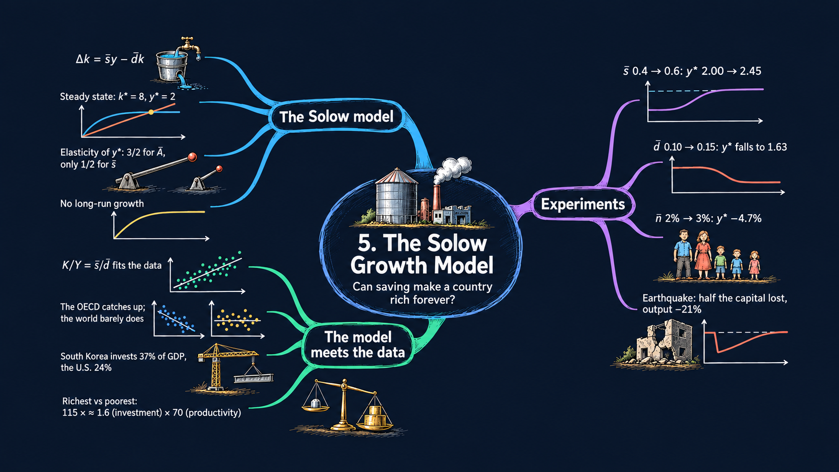
Learning goals

The Solow model explains where an economy’s capital stock comes from. By the end of this chapter you will be able to:

• draw the Solow diagram and explain why an economy moves toward a steady state;
• derive the model’s two key equations from its five assumptions, and solve them step by step for the steady-state levels of capital, output and consumption per person;
• read the comparative statics of the steady state as elasticities, and explain why productivity matters more than investment;
• derive how fast an economy grows on its way to the steady state, and how population growth changes the model;
• run experiments: a higher investment rate, a higher depreciation rate, faster population growth, or an earthquake that destroys capital;
• use the principle of transition dynamics to read cross-country data on growth and investment;
• write short Python functions, draw interactive figures with Plotly, and work with data tables in pandas.

Model overview

Picture Islandia, a small imaginary island country. Its people make one all-purpose good. Each year they can eat it, or they can turn it into tools (boats, nets, workshops) that help them make more of the good next year. Tools do not last forever: every year some of them break or rot. Will Islandia keep getting richer just by building more tools? This section answers that question with the Solow model, and we follow Islandia through every step.

NoteThe big idea

The question. Where does an economy’s capital come from, and can piling up capital make a country rich forever?

The answer in one sentence. Capital per person grows while new investment is larger than the capital that wears out, and it stops growing when the two are equal. That resting point is the steady state.

What goes in and what comes out. We choose the investment rate, the depreciation rate and productivity. The model gives back capital and output per person: in the steady state, and on the way there.

Road map.

1. The basic Solow model: the assumptions, solving the model step by step, and what the model predicts.
2. Adding population growth: what changes when Islandia’s population grows.
3. Model in code: the key results as Python functions, checked with numbers. Every later section reuses these functions.

Notation. A bar over a letter marks a parameter: a number we choose from outside the model. Letters without a bar are endogenous variables: the model determines them. In the code we simply write A, s, d and n.

Symbol	Meaning	Type
\(Y_t, K_t, L_t\)	output, capital and workers in year \(t\)	endogenous
\(C_t, I_t\)	consumption and investment in year \(t\)	endogenous
\(y_t, k_t\)	output and capital per person, \(Y_t/L_t\) and \(K_t/L_t\)	endogenous
\(\bar{A}\)	productivity	parameter
\(\bar{s}\)	investment rate: the share of output that is invested	parameter
\(\bar{d}\)	depreciation rate: the share of capital that wears out each year	parameter
\(\bar{n}\)	population growth rate (second block only)	parameter
\(\bar{K}_0, \bar{L}\)	starting capital and the size of the labor force	parameters
\(k^*, y^*\)	a star marks the steady state	endogenous
\(\Delta x_{t+1}\), \(g_x\)	the change \(x_{t+1}-x_t\), and the growth rate \(\Delta x_{t+1}/x_t\)	notation

The basic Solow model

Assumptions

Islandia makes a single good, and time runs in years, \(t = 0, 1, 2, \dots\) The model rests on five rules. Each holds in every year.

1. Production. Workers \(L_t\) use tools, the capital \(K_t\), to make output \(Y_t\). They do it with the Cobb-Douglas production function of Chapter 4:

\[Y_t = \bar{A}K_t^{1/3}L_t^{2/3}.\]

The exponents add up to one. So if Islandia doubled both its tools and its workers, it would make exactly twice as much (constant returns to scale). The exponent \(1/3\) on capital matches the share of GDP that is paid to capital.

2. Using output. Every unit of the good is either eaten or invested. Islandia has no government and does not trade with other countries:

\[C_t + I_t = Y_t.\]

This is a resource constraint. Move \(C_t\) to the right-hand side and it reads \(I_t = Y_t - C_t\): investment equals saving, the income that is not consumed.

3. Capital accumulation. Next year’s tools are this year’s tools, plus the new ones, minus those that break. A constant fraction \(\bar{d}\) of the capital stock wears out each year:

\[K_{t+1} = K_t + I_t - \bar{d}K_t \quad\Longleftrightarrow\quad \Delta K_{t+1} = I_t - \bar{d}K_t,\]

where \(\Delta K_{t+1} \equiv K_{t+1} - K_t\). Keep two words apart here. Capital is a stock: it is there at a point in time and carries over from year to year. Investment and depreciation are flows: they happen during a year and change the stock. Islandia starts with a given stock of tools, \(\bar{K}_0\).

4. Labor. The number of workers never changes: \(L_t = \bar{L}\). (We relax this in the second block.)

5. Investment. Islanders always invest the same share \(\bar{s}\) of output, a number between 0 and 1, and eat the rest:

\[I_t = \bar{s}Y_t, \qquad\text{so that}\qquad C_t = (1-\bar{s})Y_t.\]

The equation for consumption is not a sixth rule. It follows from rules 2 and 5 together.

So there are five equations for five endogenous variables, \(Y_t, K_t, L_t, C_t\) and \(I_t\):

Equation	Name	Parameters it uses
\(Y_t = \bar{A}K_t^{1/3}L_t^{2/3}\)	production function	\(\bar{A}\)
\(C_t + I_t = Y_t\)	resource constraint	none
\(\Delta K_{t+1} = I_t - \bar{d}K_t\)	capital accumulation	\(\bar{d}\), and \(\bar{K}_0\) to start
\(L_t = \bar{L}\)	labor force	\(\bar{L}\)
\(I_t = \bar{s}Y_t\)	allocation of output	\(\bar{s}\)

Markets for labor and capital do not appear in the table, but they work in the background. As in Chapter 4, the wage equals the marginal product of labor, and the rental price of capital equals the marginal product of capital. The rental price returns below, when we compute the real interest rate.

Every year is a race between new tools and broken tools. The rest of the model follows from that race.

NoteCheck your understanding

1. Islandia invests 40 percent of its output. What share does it consume, and which two rules give you the answer?

Answer

It consumes 60 percent. Rule 5 says \(I_t = 0.4\,Y_t\), and rule 2 says that what is not invested is consumed, so \(C_t = (1-0.4)Y_t = 0.6\,Y_t\).

2. Which of these are stocks and which are flows: tools, new boats built this year, nets that rot this year?

Answer

The tools are a stock, \(K_t\). The new boats are a flow (investment, \(I_t\)), and so are the rotten nets (depreciation, \(\bar{d}K_t\)). The two flows change the stock from one year to the next.

Solving the model

Step 1: from totals to per-person terms. Islanders care about their own living standards, not about the size of the whole island economy. So we work with output per person, \(y_t \equiv Y_t/L_t\), and capital per person, \(k_t \equiv K_t/L_t\). Divide the production function by \(L_t\) and use the rules for exponents (Appendix C.3):

\[y_t = \frac{\bar{A}K_t^{1/3}L_t^{2/3}}{L_t} = \bar{A}K_t^{1/3}L_t^{2/3-1} = \bar{A}K_t^{1/3}L_t^{-1/3} = \bar{A}\left(\frac{K_t}{L_t}\right)^{1/3} = \bar{A}k_t^{1/3}.\]

TipIn words

What one islander produces depends only on how many tools that islander has. And tools show diminishing returns: the exponent \(1/3\) is below one, so each extra tool adds less output than the one before. The first boat changes a fisher’s life; the tenth adds little.

Step 2: one equation for capital. Put the investment rule \(I_t = \bar{s}Y_t\) into the capital accumulation equation:

\[\underbrace{\Delta K_{t+1}}_{\text{change in capital}} = \underbrace{\bar{s}Y_t - \bar{d}K_t}_{\text{net investment}}.\]

Net investment is investment minus depreciation. Because the labor force is fixed, the change in capital per person is the change in total capital divided by \(\bar{L}\): \(\Delta k_{t+1} = (K_{t+1} - K_t)/\bar{L} = \Delta K_{t+1}/\bar{L}\). So we can divide every term by \(\bar{L}\) and get the same equation in per-person terms. Five equations have now become two:

ImportantKey result: the Solow model in two equations

\[y_t = \bar{A}k_t^{1/3} \tag{1}\]

\[\Delta k_{t+1} = \bar{s}y_t - \bar{d}k_t \tag{2}\]

Equation (1) says how much each islander makes with the tools at hand. Equation (2) says how the tools per person change: investment adds \(\bar{s}y_t\), depreciation removes \(\bar{d}k_t\).

Putting (1) into (2) leaves a single equation that carries capital per person from one year to the next:

\[\Delta k_{t+1} = \bar{s}\bar{A}k_t^{1/3} - \bar{d}k_t.\]

This equation has no simple formula for \(k_t\) in a given year. We can still learn a lot from it in three ways: draw its two terms on a chart (the Solow diagram of Fig. 1), find the level of capital at which it stops changing (next step), and simulate it year by year on a computer (Fig. 5).

Step 3: the steady state. The steady state \(k^*\) is the level of capital at which net investment is zero, \(\Delta k_{t+1} = 0\). New tools exactly replace the broken ones:

\[\bar{s}y^* = \bar{d}k^* \quad\Longrightarrow\quad \bar{s}\bar{A}(k^*)^{1/3} = \bar{d}k^*.\]

To solve for \(k^*\), divide both sides by \(\bar{d}\) and by \((k^*)^{1/3}\):

\[\frac{\bar{s}\bar{A}}{\bar{d}} = \frac{k^*}{(k^*)^{1/3}} = (k^*)^{2/3}.\]

Now raise both sides to the power \(3/2\), because \(\left((k^*)^{2/3}\right)^{3/2} = k^*\). This gives \(k^* = (\bar{s}\bar{A}/\bar{d})^{3/2}\).

For output per person, put \(k^*\) into the production function (1). The exponents multiply, \((3/2)\times(1/3) = 1/2\), and \(\bar{A}\cdot\bar{A}^{1/2} = \bar{A}^{3/2}\):

\[y^* = \bar{A}(k^*)^{1/3} = \bar{A}\left(\frac{\bar{s}\bar{A}}{\bar{d}}\right)^{1/2} = \bar{A}\cdot\bar{A}^{1/2}\left(\frac{\bar{s}}{\bar{d}}\right)^{1/2} = \left(\frac{\bar{s}}{\bar{d}}\right)^{1/2}\bar{A}^{3/2}.\]

ImportantKey result: the steady state

\[k^* = \left(\frac{\bar{s}\bar{A}}{\bar{d}}\right)^{3/2} \tag{3}\]

\[y^* = \left(\frac{\bar{s}}{\bar{d}}\right)^{1/2}\bar{A}^{3/2} \tag{4}\]

Consumption per person is what is not invested, \(c^* = (1-\bar{s})y^*\).

Islandia in numbers. With the values used throughout this notebook, \(\bar{s} = 0.4\), \(\bar{d} = 0.1\) and \(\bar{A} = 1\), we get \(\bar{s}\bar{A}/\bar{d} = 4\). So \(k^* = 4^{3/2} = 8\), \(y^* = 4^{1/2} = 2\) and \(c^* = 0.6 \times 2 = 1.2\).

TipIn words: why Islandia settles down

Suppose Islandia has few tools. Each new tool adds a lot of output, so investment is large, and the stock of tools grows. But as tools pile up, diminishing returns kick in. Each extra tool adds less output, and so less investment, than the one before. Each extra tool still adds the same amount \(\bar{d}\) to depreciation, though. Sooner or later the broken tools catch up with the new ones, and accumulation stops at \(k^*\).

The steady state also gives us four more results. Each one takes a single line of algebra, and each is used later in the notebook.

Step 4: the capital-output ratio. Divide both sides of the steady-state condition \(\bar{s}y^* = \bar{d}k^*\) by \(\bar{d}y^*\). Since \(k/y = (K/L)/(Y/L) = K/Y\),

\[\frac{K^*}{Y^*} = \frac{k^*}{y^*} = \frac{\bar{s}}{\bar{d}}. \tag{5}\]

Productivity drops out of this ratio completely. Islandia, with \(\bar{s} = 0.4\) and \(\bar{d} = 0.1\), holds tools worth 4 years of output. Fig. 3 puts this prediction to the test with data.

Step 5: how fast the economy grows on the way. Divide equation (2) by \(k_t\) to get the growth rate of capital per person, then use the production function:

\[g_{k,t} \equiv \frac{\Delta k_{t+1}}{k_t} = \bar{s}\frac{y_t}{k_t} - \bar{d} = \bar{s}\bar{A}k_t^{-2/3} - \bar{d}.\]

The steady-state condition of step 3 says \(\bar{s}\bar{A} = \bar{d}(k^*)^{2/3}\). Substituting it gives a formula that depends only on the distance to the steady state:

\[g_{k,t} = \bar{d}\left[\left(\frac{k^*}{k_t}\right)^{2/3} - 1\right]. \tag{6}\]

Output per person grows about a third as fast as capital per person, \(g_{y,t} \approx \tfrac{1}{3}g_{k,t}\), by the growth rule for powers (Appendix C.5).

TipIn words: the principle of transition dynamics

The farther Islandia is below its steady state, in percentage terms, the faster it grows. Above the steady state, it shrinks. With \(\bar{d} = 0.1\), an Islandia with half its steady-state tools adds \(0.1\times(2^{2/3}-1) \approx 5.9\%\) to its capital per person in a year. At 95 percent of the steady state, the rate falls to about \(0.35\%\). Equation (6) is the algebra behind this principle of transition dynamics.

Step 6: comparing two countries. Write equation (4) for Islandia and for a second country with the same depreciation rate, and divide one by the other. The \(\bar{d}\) terms cancel:

\[\frac{y^*_1}{y^*_2} = \left(\frac{\bar{A}_1}{\bar{A}_2}\right)^{3/2}\times\left(\frac{\bar{s}_1}{\bar{s}_2}\right)^{1/2}. \tag{7}\]

The gap in long-run incomes splits into a productivity part and an investment part. We use this formula for rich and poor countries in Fig. 3, and for Korea and the United States in Fig. 10.

Step 7: the real interest rate. The real interest rate is what one unit of output earns when it is saved for a year. In Islandia, a saved unit becomes a tool, and a tool earns its rental price, the marginal product of capital. With \(y = \bar{A}k^{1/3}\), that marginal product is \(\frac{1}{3}\bar{A}k^{-2/3} = \frac{1}{3}\,y/k\) (Chapter 4). In the steady state, equation (5) gives \(y^*/k^* = \bar{d}/\bar{s}\), so

\[r^* = \frac{1}{3}\cdot\frac{\bar{d}}{\bar{s}}.\]

For Islandia, \(r^* = 0.1/(3\times0.4) \approx 8.3\%\). A country that invests more ends up with more tools per unit of output, and so earns less on its last tool.

Diminishing returns make investment fall behind depreciation, so capital per person settles at a steady state.

NoteCheck your understanding

1. Islandia doubles its investment rate from 0.4 to 0.8, with \(\bar{d} = 0.1\) and \(\bar{A} = 1\). What are the new \(k^*\) and \(y^*\)? By what percentage does output per person rise?

Answer

Now \(\bar{s}\bar{A}/\bar{d} = 8\). Equation (3) gives \(k^* = 8^{3/2} \approx 22.6\), and equation (4) gives \(y^* = 8^{1/2} \approx 2.83\). Output per person rises from 2 to 2.83, by about 41 percent. Doubling the investment rate is far from doubling income.

2. Islandia starts with very few tools, \(\bar{K}_0\) small. Does that change its steady state?

Answer

No. \(\bar{K}_0\) does not appear in equations (3) and (4). The starting point decides only the path: a poorer start means a longer climb, at a faster pace (equation 6), to the same \(k^*\).

What the model predicts

Comparative statics. What happens to the steady state when a parameter changes? Take logs of equations (3) and (4) (Appendix C.4):

\[\ln k^* = \tfrac{3}{2}\ln\bar{s} + \tfrac{3}{2}\ln\bar{A} - \tfrac{3}{2}\ln\bar{d}, \qquad \ln y^* = \tfrac{1}{2}\ln\bar{s} + \tfrac{3}{2}\ln\bar{A} - \tfrac{1}{2}\ln\bar{d}.\]

Each coefficient is an elasticity: the percentage change in \(k^*\) or \(y^*\) when that parameter rises by 1 percent.

A 1% rise in …	changes \(k^*\) by	changes \(y^*\) by	Which curve of the Solow diagram moves
investment rate \(\bar{s}\)	\(+1.5\%\)	\(+0.5\%\)	the investment curve rotates up
productivity \(\bar{A}\)	\(+1.5\%\)	\(+1.5\%\)	the investment curve (and the output curve) rotate up
depreciation rate \(\bar{d}\)	\(-1.5\%\)	\(-0.5\%\)	the depreciation line rotates up
labor force \(\bar{L}\)	\(0\)	\(0\)	none: per-person values do not depend on scale

Because the formulas are powers, these numbers hold for any parameter values. For large changes, use the ratios directly. Doubling \(\bar{s}\) multiplies \(y^*\) by \(2^{1/2} \approx 1.41\), while doubling \(\bar{A}\) multiplies it by \(2^{3/2} \approx 2.83\). A larger labor force raises total capital \(K^* = \bar{L}k^*\) and total output \(Y^* = \bar{L}y^*\) one for one, but leaves the per-person values unchanged.

Why productivity matters more than investment. In the production model of Chapter 4, capital per person was fixed at \(\bar{k}\), and output per person was \(y^* = \bar{A}\bar{k}^{1/3}\): the exponent on \(\bar{A}\) was 1. In the Solow model it is \(3/2\). To see where the extra \(1/2\) comes from, write \(y^* = \bar{A}\times(k^*)^{1/3}\):

• Direct effect. Better know-how lets Islanders make more with the same tools (the exponent 1 on \(\bar{A}\)).
• Capital effect. More output means more investment, so more tools, so more output again. This adds another \(1/2\), since \((k^*)^{1/3} = (\bar{s}\bar{A}/\bar{d})^{1/2}\).

The investment rate works only through the second channel, and diminishing returns keep its exponent at \(1/2\). So differences in investment explain only a small part of the income gaps between countries. Differences in productivity explain most of them.

No long-run growth. In the steady state, \(k\), \(y\) and \(c = (1-\bar{s})y\) are all constant. Building tools raises Islandia’s output per person for a while, during the transition, but diminishing returns bring it to a halt. Capital accumulation alone cannot explain the steady growth in living standards that we see in the data. Chapter 6 adds new ideas to explain it.

Transition dynamics. From any starting capital \(\bar{k}_0 > 0\), the economy moves toward \(k^*\). It grows when \(k_t < k^*\) and shrinks when \(k_t > k^*\), faster the farther away it is (equation 6). Three kinds of events show this at work in the notebook:

• A permanent change in \(\bar{s}\), \(\bar{A}\) or \(\bar{d}\) moves the steady state, and the economy grows or shrinks on its way to the new one (Figs. 4–7).
• A one-time loss of capital, such as an earthquake or a war, leaves the steady state where it was. The economy simply grows back, fastest right after the shock (Figs. 12–13).
• Across countries, those far below their steady states should grow faster than those close to theirs (Figs. 8–9).

Saving more makes a country richer, but only for a while and only by a little. Productivity does far more.

NoteCheck your understanding

1. Two countries have the same investment and depreciation rates, but the first is twice as productive. How many times richer is it in the steady state?

Answer

By equation (7), \(y^*_1/y^*_2 = 2^{3/2} \approx 2.83\). It is almost three times richer: twice from the direct effect, and about 1.41 times more from the extra capital that productivity pays for.

2. A storm destroys half of Islandia’s tools. Does its steady state change? How fast does its capital per person grow in the year after the storm?

Answer

The steady state does not change: \(\bar{s}\), \(\bar{A}\) and \(\bar{d}\) are the same. Islandia is now at half its steady-state capital, so by equation (6) its capital per person grows by about \(0.1\times(2^{2/3}-1) \approx 5.9\%\) in that year, much faster than before the storm.

Adding population growth

Assumptions

Keep every rule above except the fourth. Islandia’s population, and with it the number of workers, now grows at a constant rate \(\bar{n}\):

\[\frac{\Delta L_{t+1}}{L_t} = \bar{n}.\]

Solving the model

The production function per person, equation (1), stays the same, because dividing by \(L_t\) works the same way in every year. What changes is the accumulation equation. Capital per person \(k_t = K_t/L_t\) now changes for two reasons: the tools change, and so does the number of people who share them.

The growth rate of a ratio is the growth rate of the numerator minus that of the denominator, \(g_k = g_K - g_L\) (Appendix C.5; the rule is exact in continuous time and a close approximation for yearly data). Step by step:

\[\frac{\Delta k_{t+1}}{k_t} = \frac{\Delta K_{t+1}}{K_t} - \frac{\Delta L_{t+1}}{L_t} = \frac{\bar{s}Y_t - \bar{d}K_t}{K_t} - \bar{n} = \bar{s}\frac{Y_t}{K_t} - \bar{d} - \bar{n} = \bar{s}\frac{y_t}{k_t} - (\bar{n}+\bar{d}).\]

The last step uses \(Y/K = y/k\). Multiplying both sides by \(k_t\) gives equation (8) in the box below. Setting \(\Delta k_{t+1} = 0\) in it gives \(\bar{s}\bar{A}(k^*)^{1/3} = (\bar{n}+\bar{d})k^*\), and the steady state follows exactly as in step 3, with \(\bar{n}+\bar{d}\) in place of \(\bar{d}\).

ImportantKey result: the Solow model with population growth

\[\Delta k_{t+1} = \bar{s}y_t - (\bar{n}+\bar{d})k_t \tag{8}\]

\[k^* = \left(\frac{\bar{s}\bar{A}}{\bar{n}+\bar{d}}\right)^{3/2} \qquad\text{and}\qquad y^* = \bar{A}^{3/2}\left(\frac{\bar{s}}{\bar{n}+\bar{d}}\right)^{1/2} \tag{9}\]

Islandia in numbers. With \(\bar{s} = 0.4\), \(\bar{n} = 0.02\) and \(\bar{d} = 0.08\) (the starting values of Fig. 11), \(\bar{n}+\bar{d} = 0.10\), so \(k^* = 8\) and \(y^* = 2\), as before.

TipIn words

Compared with equation (2), the depreciation rate \(\bar{d}\) is replaced by \(\bar{n}+\bar{d}\). Islandia’s investment now has two jobs: replace the tools that break, and equip each newcomer with as many tools as everyone else. Only what is left after both jobs raises capital per person.

What the model predicts

• Still no long-run growth per person. The economy again converges to constant \(k^*\) and \(y^*\).
• Faster population growth lowers income per person. In logs, \(\ln y^* = \frac{3}{2}\ln\bar{A} + \frac{1}{2}\ln\bar{s} - \frac{1}{2}\ln(\bar{n}+\bar{d})\). A 1% rise in \(\bar{n}+\bar{d}\) lowers \(y^*\) by 0.5%. Raising \(\bar{n}\) from 0.02 to 0.03 raises \(\bar{n}+\bar{d}\) from 0.10 to 0.11 and lowers \(y^*\) by the factor \((0.10/0.11)^{1/2} \approx 0.95\), about 5 percent.
• Total GDP grows. \(Y_t = y_tL_t\), so \(g_Y = g_y + g_L\) by the growth rule for a product. In the steady state \(g_y = 0\), so total output, total capital and population all grow at the rate \(\bar{n}\).
• Size does not matter per person. With constant returns to scale, an economy with 100 times more people and 100 times more tools has the same output per person. That is why population growth makes Islandia bigger, but not richer per person. Chapter 6 shows how ideas change this.

Every newcomer needs tools too, so faster population growth works just like faster depreciation.

NoteCheck your understanding

1. Start from \(\bar{s} = 0.4\), \(\bar{d} = 0.1\), \(\bar{A} = 1\) and \(\bar{n} = 0\). Population growth rises to \(\bar{n} = 0.05\). What happens to \(y^*\)? And at what rate does Islandia’s total GDP grow in the new steady state?

Answer

Now \(\bar{n}+\bar{d} = 0.15\), so by equation (9) \(y^* = (0.4/0.15)^{1/2} \approx 1.63\), down from 2: about 18 percent lower. In the new steady state output per person is constant, so total GDP grows at the rate of population, 5 percent a year.

NoteRecap

• Two equations hold the whole model: production per person, \(y_t = \bar{A}k_t^{1/3}\), and capital accumulation, \(\Delta k_{t+1} = \bar{s}y_t - \bar{d}k_t\) (the Solow diagram of Fig. 1).
• The steady state is where investment just covers depreciation: \(k^* = (\bar{s}\bar{A}/\bar{d})^{3/2}\) and \(y^* = (\bar{s}/\bar{d})^{1/2}\bar{A}^{3/2}\).
• Productivity matters more than investment: the elasticity of \(y^*\) is \(3/2\) for \(\bar{A}\), but only \(1/2\) for \(\bar{s}\) (the data test in Fig. 3).
• No long-run growth: capital accumulation raises income only during the transition (Fig. 5).
• Transition dynamics: an economy with a large gap to its steady state grows fast, and slows down as the gap closes (Fig. 8, Fig. 13).
• Population growth acts like extra depreciation, \(\bar{n}+\bar{d}\), and lowers \(y^*\) (Fig. 11).

Model in code

Now we turn the Key results into Python. The section has four parts: the setup (folded, because it is the same in every chapter), the model as functions, numerical checks of the Key results, and the drawing tools that the figures use (folded too). Run its cells once, in order. Every later section of the notebook reuses them.

Setup

Run the setup cells once, before anything else. They load the Python libraries, give every chart the same look, store the address of the chapter’s data and define two helpers that only the book website needs. You can use the notebook without reading them; open the box if you are curious.

NoteShow the setup code

The first cell loads the libraries and sets the look of the charts. Its comments explain each step.

# @title Setup: libraries, chart colors and the data location
# Text after a "#" is a comment: Python ignores it, it is there for human readers.

# Step 1: load the libraries. `import` loads a library, a toolbox written by
# other people, and `as np` gives it a short nickname, so the code stays short.
import numpy as np                              # numbers and arrays
import pandas as pd                             # data tables
import plotly.express as px                     # quick charts from data tables
import plotly.graph_objects as go               # charts built piece by piece
import plotly.io as pio                         # settings shared by every chart
from plotly.subplots import make_subplots       # several panels in one figure
# sliders and buttons for the interactive figures
from ipywidgets import interact, interact_manual, FloatSlider, ToggleButtons, Dropdown, fixed

# Step 2: one light blue/green look for every chart
BLUE, TEAL, GREEN, GRAY = "#16528c", "#008070", "#7fb23a", "#8a96a3"
pio.templates.default = "plotly_white"
# the same chart size in Colab and on the website
pio.templates["plotly_white"].layout.update(width=860, height=480)
px.defaults.color_discrete_sequence = [BLUE, TEAL, GREEN, "#5aa0d8", "#0b4f47"]
WIDE = {"description_width": "initial"}         # show the full slider labels

# Step 3, Colab only: let Plotly charts appear inside the interactive widgets.
# `try` runs the indented lines; if the import fails (we are not in Colab),
# `except` skips them.
try:
    import google.colab
    google.colab.output.enable_custom_widget_manager()
except ImportError:
    pass                                        # not running in Colab: nothing to do

# Step 4: the data files of this chapter live in the book's GitHub repository
DATA_URL = "https://raw.githubusercontent.com/quarcs-lab/macro102-site/main/data/ch05/"

The website cannot run Python, so each interactive figure also gets a version with a precomputed slider. The next two helpers build those versions. Run them and move on.

# @title Helper for the website versions (run this cell; you do not need to read it)
def slider_figure(make_figure, name, values, start, label=None):
    """Join precomputed versions of a figure with one slider (the website cannot run Python).

    Arguments
        make_figure : the function that draws the figure, e.g. solow_diagram
        name        : the argument the slider moves, e.g. "s"
        values      : the values of that argument to precompute
        start       : the value shown first
        label       : the slider's label (the argument name if None)
    Returns
        one Plotly figure with all versions and a slider that shows one at a time
    """
    # Step 1: draw the figure once for every value
    figures = [make_figure(**{name: v}) for v in values]
    first = values.index(start)
    # Step 2: copy every curve into one figure; only the start value's are visible
    fig = go.Figure(layout=figures[first].layout)
    owner = []                          # which precomputed figure each trace is from
    for i, f in enumerate(figures):
        for trace in f.data:
            trace.visible = (i == first)
            fig.add_trace(trace)
            owner.append(i)
    # Step 3: one slider step per value: its curves, title, labels and shapes
    steps = []
    for i, f in enumerate(figures):
        layout = {"title": f.layout.title.to_plotly_json(),
                  "annotations": [a.to_plotly_json() for a in f.layout.annotations],
                  "shapes": [s.to_plotly_json() for s in f.layout.shapes]}
        visible = [o == i for o in owner]
        steps.append(dict(method="update", label=str(values[i]), args=[{"visible": visible}, layout]))
    fig.update_layout(sliders=[dict(active=first, steps=steps, pad=dict(t=60),
                                    currentvalue=dict(prefix=(label or name) + " = "))])
    return fig

# @title Helper for the website versions with many countries (run this cell; you do not need to read it)
def country_menu(fig, shown, regions, label="Textbook countries"):
    """Draw the countries in `shown` and put every other country one click away in the legend.

    With more than 40 countries, a menu above the plot chooses the region whose countries the legend lists.
    Traces that are not countries stay as they are.

    Arguments
        fig     : a Plotly figure with one trace per country
        shown   : the countries drawn at the start
        regions : maps each country to its region
        label   : the name of the first menu entry
    Returns
        the same figure, with the visibility set and, for many countries, the region menu
    """
    # Step 1: the menu entries, the textbook countries and then one entry per region
    # the traces that are countries, and each of their regions once, A to Z
    countries = [trace.name for trace in fig.data if trace.name in regions]
    groups = [label] + sorted(set(regions[name] for name in countries))
    if len(countries) <= 40:
        groups = [None]                     # a short legend lists every country at once
    # Step 2: for each entry, which traces are drawn, in the legend only, or hidden
    buttons = []
    for group in groups:
        visible = []
        for trace in fig.data:
            if trace.name in shown:
                visible.append(True)                    # a textbook country: drawn
            elif trace.name not in regions:
                visible.append(True if trace.visible is None else trace.visible)   # not a country: as it was
            elif group is None or regions[trace.name] == group:
                visible.append("legendonly")    # in this region: a click away
            else:
                visible.append(False)                   # another region: hidden
        buttons.append(dict(label=group, method="restyle", args=[{"visible": visible}]))
    # Step 3: start with the first entry, and add the menu when there is more than one
    for trace, v in zip(fig.data, buttons[0]["args"][0]["visible"]):
        trace.visible = v
    if len(groups) > 1:
        menu = dict(type="dropdown", buttons=buttons, x=1, xanchor="right", y=1.02, yanchor="bottom")
        fig.update_layout(updatemenus=list(fig.layout.updatemenus) + [menu], margin=dict(t=110))
    return fig

The model as functions

Two Key results hold the whole model: the production function, equation (1), and the steady state, equations (3), (4) and (9). We write each one as a Python function: a named recipe that takes inputs and gives back a result. The first function is output per person.

# `def` creates a function. Its inputs are the arguments in parentheses.
# `A=1.0` gives A a default value, used whenever we do not pass one.
# The text in triple quotes describes the function.
def output(k, A=1.0):
    """Output per person, from the production function.

    Equation (1):  y = A k^(1/3)

    Arguments
        k : capital per person
        A : productivity, A-bar (1 unless we pass another value)
    Returns
        output per person, y
    """
    # `return` gives back the result; `**` means "to the power of"
    return A * k ** (1 / 3)

The steady state is where investment just covers depreciation. Solving equation (2) for that point gives \(k^*\), and putting \(k^*\) into the production function gives \(y^*\). The argument n is population growth, which adds to depreciation (equation 9). It is 0 unless we pass another value, so the same functions serve the basic model and the model with population growth in Fig. 11.

def steady_state_k(s, d, A=1.0, n=0.0):
    """Steady-state capital per person, k*.

    Equation (3), or (9) with population growth:  k* = (s A / (n + d))^(3/2)

    Arguments
        s : investment rate, s-bar
        d : depreciation rate, d-bar
        A : productivity, A-bar
        n : population growth rate, n-bar (0 in the basic model)
    Returns
        steady-state capital per person, k*
    """
    # investment s A k^(1/3) equals (n + d) k exactly at k*; solving for k gives:
    return (s * A / (n + d)) ** (3 / 2)


def steady_state_y(s, d, A=1.0, n=0.0):
    """Steady-state output per person, y*.

    Equation (4), or (9) with population growth:  y* = A^(3/2) (s / (n + d))^(1/2)

    Arguments
        s : investment rate, s-bar
        d : depreciation rate, d-bar
        A : productivity, A-bar
        n : population growth rate, n-bar (0 in the basic model)
    Returns
        steady-state output per person, y*
    """
    # the same as output(steady_state_k(s, d, A, n), A), written as one formula
    return A ** (3 / 2) * (s / (n + d)) ** (1 / 2)

Checking the key results

The formulas came from algebra. Now we check them with numbers, one Key result at a time, using Islandia’s values \(\bar{s}=0.4\), \(\bar{d}=0.1\) and \(\bar{A}=1\). First the steady state itself: the formula for \(y^*\) and the production function applied to \(k^*\) must give the same number, and so must both sides of equation (5).

# Islandia's steady state, from equation (3) and then equation (1)
k_star = steady_state_k(s=0.4, d=0.1)
y_star = output(k_star)

# An f-string, f"... {value:.2f}", puts a value into the text;
# ":.2f" means "two decimals".
print(f"Steady-state capital per person k* = {k_star:.2f}")
print(f"Steady-state output per person  y* = {y_star:.2f}")
# equation (4) must give the same y* as the line above
print(f"Check with equation (4):        y* = {steady_state_y(s=0.4, d=0.1):.2f}")
# consumption is what is not invested, c* = (1 - s) y*
print(f"Consumption per person          c* = {(1 - 0.4) * y_star:.2f}")
# both sides of equation (5), K/Y = s/d
print(f"Capital-output ratio, eq. (5): k*/y* = {k_star / y_star:.2f}   and s/d = {0.4 / 0.1:.2f}")
print(f"Real interest rate (1/3)(d/s):   r* = {100 * 0.1 / (3 * 0.4):.1f}%")

Steady-state capital per person k* = 8.00
Steady-state output per person  y* = 2.00
Check with equation (4):        y* = 2.00
Consumption per person          c* = 1.20
Capital-output ratio, eq. (5): k*/y* = 4.00   and s/d = 4.00
Real interest rate (1/3)(d/s):   r* = 8.3%

Check 1: Islandia really converges to \(k^*\). We start Islandia with very few tools and apply equation (2) for 300 years, one year at a time. Capital should approach the \(k^*\) of the formula.

# Step 1: start far below the steady state
k = 1.0

# Step 2: apply equation (2) once a year. `range(300)` counts 0, 1, ..., 299,
# so the `for` loop runs its indented lines 300 times.
# `if year in (10, 50, 100)` is true only in those years.
for year in range(300):
    if year in (10, 50, 100):
        print(f"Year {year:3d}: k = {k:.3f}")
    # new k = old k + investment - depreciation
    k = k + 0.4 * output(k) - 0.1 * k

# Step 3: compare the end point with the formula
print(f"Year 300: k = {k:.3f}   (formula: k* = {steady_state_k(s=0.4, d=0.1):.3f})")

Year  10: k = 3.883
Year  50: k = 7.709
Year 100: k = 7.991
Year 300: k = 8.000   (formula: k* = 8.000)

Check 2: the elasticities. We raise each parameter by 1 percent and see by what percentage \(y^*\) changes. The comparative-statics table predicts \(+0.5\%\) for \(\bar{s}\), \(+1.5\%\) for \(\bar{A}\) and \(-0.5\%\) for \(\bar{d}\).

# Step 1: y* at Islandia's values
base = steady_state_y(s=0.4, d=0.1, A=1.0)

# Step 2: y* with one parameter 1% higher, relative to the base (0.005 = 0.5%)
change_s = steady_state_y(s=0.4 * 1.01, d=0.1, A=1.0) / base - 1
change_A = steady_state_y(s=0.4, d=0.1, A=1.0 * 1.01) / base - 1
change_d = steady_state_y(s=0.4, d=0.1 * 1.01, A=1.0) / base - 1

# Step 3: show them in percent; ":+.3f" shows the sign and three decimals
print(f"1% higher s: y* changes by {100 * change_s:+.3f}%")
print(f"1% higher A: y* changes by {100 * change_A:+.3f}%")
print(f"1% higher d: y* changes by {100 * change_d:+.3f}%")

1% higher s: y* changes by +0.499%
1% higher A: y* changes by +1.504%
1% higher d: y* changes by -0.496%

The answers are close to 0.5, 1.5 and −0.5 but not exact. An elasticity describes very small changes, and 1 percent is small but not zero.

Check 3: the speed of transition. Equation (6) says that the growth rate of capital depends only on how far \(k_t\) is from \(k^*\). We compare it with the growth rate computed directly from equation (2). The 50 percent row is Islandia right after the storm in What the model predicts.

# Islandia's steady state, the benchmark for "how far from k*"
k_star = steady_state_k(s=0.4, d=0.1)

# For capital at 50%, 95% and 150% of the steady state, compute the growth
# rate of k in two ways; ":.0%" shows a share as a percentage
for share in (0.5, 0.95, 1.5):
    k = share * k_star
    direct = (0.4 * output(k) - 0.1 * k) / k        # equation (2): net investment / k
    formula = 0.1 * ((k_star / k) ** (2 / 3) - 1)   # equation (6)
    print(f"k = {share:.0%} of k*: growth of k = {100 * direct:+.2f}% (direct), {100 * formula:+.2f}% (eq. 6)")

k = 50% of k*: growth of k = +5.87% (direct), +5.87% (eq. 6)
k = 95% of k*: growth of k = +0.35% (direct), +0.35% (eq. 6)
k = 150% of k*: growth of k = -2.37% (direct), -2.37% (eq. 6)

Check 4: population growth. With \(\bar{n} = 0.02\) and \(\bar{d} = 0.08\), equation (9) gives the same steady state as \(\bar{n} = 0\) and \(\bar{d} = 0.1\), because only \(\bar{n}+\bar{d}\) matters. Faster population growth, 3 percent, should lower \(y^*\) by about 5 percent.

# y* with 2% and with 3% population growth (equation 9); n + d is 0.10 and then 0.11
y_n2 = steady_state_y(s=0.4, d=0.08, n=0.02)
y_n3 = steady_state_y(s=0.4, d=0.08, n=0.03)
print(f"n = 2%: y* = {y_n2:.3f}")
print(f"n = 3%: y* = {y_n3:.3f}   ({100 * (y_n3 / y_n2 - 1):+.1f}%)")

n = 2%: y* = 2.000
n = 3%: y* = 1.907   (-4.7%)

Drawing tools

The Solow diagrams of the figures share four small tools: one draws a curve and writes its name on the plot, one draws an arrow along the capital axis, and two set up the axes. Run them and move on, or open the box to see how they work.

NoteShow the drawing tools

As in the textbook, every curve of a Solow diagram carries its name on the plot, right after its last point inside the axes, so the diagrams need no legend. add_curve draws one curve and writes its name. If the name of another curve already sits close by, it leaves the name out, so that two names never overlap.

# @title Drawing tool: a curve with its name on the plot
def add_curve(fig, k, y, label, color, y_max, dash="solid", row=None, col=None):
    """Draw one curve of a Solow diagram and write its name at its last point inside the axes.

    Arguments
        fig      : the figure to draw on
        k, y     : the points of the curve (arrays)
        label    : the curve's name, e.g. "Investment, s·y"
        color    : its color, e.g. TEAL
        y_max    : the top of the vertical axis
        dash     : "solid" or "dash"
        row, col : the panel to draw in (only for figures with two panels, Figs. 5 and 7)
    """
    # Step 1: keep the part of the curve below the top of the axes. `y <= y_max`
    # gives True or False for each point; `k[inside]` keeps the points where it is True.
    inside = y <= y_max
    fig.add_trace(go.Scatter(x=k[inside], y=y[inside], name=label, mode="lines",
                             line=dict(color=color, width=3, dash=dash)), row=row, col=col)
    # [-1] is the last element: the last point inside the axes
    k_end, y_end = k[inside][-1], y[inside][-1]

    # Step 2: is another name already close by? (`abs` is the absolute value)
    for old in fig.layout.annotations:
        if old.showarrow is False and old.xref != "paper":
            if abs(old.y - y_end) < y_max / 12 and abs(old.x - k_end) < k[-1] / 3:
                # yes: a bare `return` leaves the function early, without a name
                return

    # Step 3: write the name right after the curve's last point: level with it when
    # the curve reaches the right edge, just below the top if it leaves through the top
    if inside[-1]:
        anchor = "middle"
    else:
        anchor = "top"
    fig.add_annotation(x=k_end, y=y_end, text=label, showarrow=False, xanchor="left", yanchor=anchor,
                       xshift=5, font=dict(color=color, size=13), row=row, col=col)

add_arrow shows where capital moves: from a starting point toward the steady state.

# @title Drawing tool: an arrow along the capital axis
def add_arrow(fig, k_from, k_to, height):
    """Draw an arrow along the k-axis from k_from to k_to (none if the two are the same).

    Arguments
        fig    : the figure to draw on
        k_from : where capital starts
        k_to   : where capital goes
        height : the height of the arrow on the vertical axis
    """
    # draw it only if the two points are visibly apart
    if abs(k_to - k_from) > 0.1:
        fig.add_annotation(x=k_to, y=height, ax=k_from, ay=height, xref="x", yref="y", axref="x", ayref="y",
                           showarrow=True, arrowhead=3, arrowwidth=2, arrowcolor=GREEN)

The axes of each diagram are fixed, so that you can see the curves move. Only when an extreme slider setting would push a steady state off the chart does axis_end widen an axis, by doubling it until the point fits.

# @title Drawing tools: fixed axes that widen only when needed
def axis_end(top, end):
    """The end of a fixed axis, doubled until the highest point fits on the chart.

    Arguments
        top : the highest point to show, e.g. k*
        end : the usual end of the axis
    Returns
        the end of the axis: `end`, or a doubled value if `top` would fall off
    """
    # a `while` loop repeats as long as its condition is true: here, as long as
    # the point would fall off the chart, double the axis
    while top > 0.95 * end:
        end = 2 * end
    return end


def k_axis(k_end):
    """The k-axis of a Solow diagram, from 0 to k_end, with round ticks and none at 0 (the corner).

    Arguments
        k_end : the end of the axis (from axis_end)
    Returns
        the axis settings, for fig.update_layout(xaxis=...)
    """
    # `//` divides and drops the remainder; ticks 5 apart on the usual axis, 0 to 20
    step = 5 * (k_end // 20)
    # list(range(5, 21, 5)) is [5, 10, 15, 20], the ticks of the usual axis
    return dict(title="Capital per person, k", range=[0, k_end], tickvals=list(range(step, k_end + 1, step)))

The Solow diagram and the steady state

We start with the diagram that solves the model: investment and depreciation against capital per person. Where the two curves cross, the economy is in its steady state.

Fig. 1: The Solow diagram

Goal. See why the economy moves toward the steady state \(k^*\) from any starting point \(k_0\).

The Solow diagram plots the two parts of equation (2) against capital per person \(k\):

• investment \(\bar{s}y = \bar{s}\bar{A}k^{1/3}\), which is a curve because of diminishing returns;
• depreciation \(\bar{d}k\), which is a straight line.

When investment is above depreciation, net investment is positive, so capital grows. When it is below, capital shrinks. Where the two cross, capital stops changing: that point is the steady state \(k^*\). In the figure, the green bar at a starting point \(k_0\) is net investment, the gap between the two curves, and the green arrow on the horizontal axis shows where capital moves.

First we compute the two numbers the figure reports. solow_point finds the steady state \(k^*\) and the net investment at the starting point \(k_0\): the height of the green bar.

def solow_point(s, d, A, k0):
    """The steady state, and net investment at a starting point (Fig. 1).

    Equations (3) and (2):  k* = (s A / d)^(3/2),  net investment = s A k0^(1/3) - d k0

    Arguments
        s  : investment rate, s-bar
        d  : depreciation rate, d-bar
        A  : productivity, A-bar
        k0 : starting capital per person, k0
    Returns
        k_star : steady-state capital per person, k*
        net    : net investment at k0 (positive: capital grows; negative: it shrinks)
    """
    k_star = steady_state_k(s, d, A)
    # investment minus depreciation at k0: the change in capital, equation (2)
    net = s * output(k0, A) - d * k0
    return k_star, net

# @title Drawing code: Fig. 1, the Solow diagram
def solow_diagram(s=0.4, d=0.1, A=1.0, k0=2.7):
    """The Solow diagram: investment s*y and depreciation d*k against k.

    Draws Fig. 1 (adapted from Fig. 5.1 in Jones), with the net investment bar at k0
    and an arrow that shows where capital moves.

    Arguments
        s  : investment rate, s-bar
        d  : depreciation rate, d-bar
        A  : productivity, A-bar
        k0 : starting capital per person, k0
    Returns
        a Plotly figure
    """
    # Step 1: the numbers of the figure (solow_point)
    k_star, net = solow_point(s, d, A, k0)
    # rounded for the title; + 0.0 turns "-0.000" into "0.000"
    net = round(net, 3) + 0.0

    # Step 2: fixed axes, so that you can see the curves move when a parameter
    # changes. 0 to 20, wider only when k* would fall off the chart
    k_end = axis_end(k_star, 20)
    # `np.linspace(0, k_end, 200)`: 200 evenly spaced values of k from 0 to k_end,
    # the points at which we draw the curves
    k = np.linspace(0, k_end, 200)
    # the top of the vertical axis, higher only when needed
    y_max = axis_end(d * max(k0, k_star), 2.2)

    # Step 3: `go.Figure()` starts an empty chart, and each `add_trace` adds one
    # curve or set of points (`add_curve` calls it and writes the curve's name)
    fig = go.Figure()
    add_curve(fig, k, s * output(k, A), "Investment, s·y", TEAL, y_max)
    add_curve(fig, k, d * k, "Depreciation, d·k", BLUE, y_max)
    # the green bar: net investment at k0, from d*k0 up to s*y0
    fig.add_trace(
        go.Scatter(
            x=[k0, k0],
            y=[d * k0, s * output(k0, A)],
            name="Net investment at k0",
            mode="lines",
            line=dict(color=GREEN, width=5),
        )
    )
    # the steady state: a black dot labeled k*
    fig.add_trace(
        go.Scatter(
            x=[k_star],
            y=[d * k_star],
            name="Steady state",
            mode="markers+text",
            text=["k*"],
            textposition="top left",
            marker=dict(color="black", size=11),
        )
    )
    # an arrow on the k-axis (`add_arrow` draws it with `add_annotation`, which
    # writes a piece of text or an arrow on the chart): from k0 toward k*
    add_arrow(fig, k0, k_star, 0.05)

    # Step 4: the title reports k* and net investment at k0
    fig.update_layout(
        title=f"k* = {k_star:.2f}   |   net investment at k0 = {k0:.1f}: {net:+.3f}",
        xaxis=k_axis(k_end),
        yaxis=dict(title="Investment and depreciation", range=[0, y_max]),
        showlegend=False,
        margin=dict(r=150),            # room on the right for the curve names
    )
    return fig

Now the interactive version. Move the sliders and watch where the curves cross.

# Fig. 1 with sliders. `interact` turns each argument of solow_diagram into a
# slider, and draws the figure again every time you move one. The `;` at the end
# only hides an extra line of text.
interact(
    solow_diagram,
    s=FloatSlider(value=0.4, min=0.1, max=0.6, step=0.05,
                  description="investment rate s", style=WIDE),
    d=FloatSlider(value=0.1, min=0.05, max=0.2, step=0.01,
                  description="depreciation rate d", style=WIDE),
    A=FloatSlider(value=1.0, min=0.5, max=1.5, step=0.1,
                  description="productivity A", style=WIDE),
    k0=FloatSlider(value=2.7, min=0.5, max=19.5, step=0.1,
                   description="starting capital k0", style=WIDE),
);

# @title Website version: Fig. 1 with a precomputed slider for the investment rate
# one picture of Fig. 1 per value of s; the slider shows one at a time
slider_figure(
    solow_diagram,
    "s",
    [0.2, 0.25, 0.3, 0.35, 0.4, 0.45, 0.5, 0.55, 0.6],     # the values of s
    start=0.4,
    label="investment rate s",
)

Source. Adapted from Fig. 5.1 in Jones (2024), Macroeconomics, 6th ed.

What to notice.

• At \(k_0 = 2.7\) the green bar points up: investment exceeds depreciation, so capital rises toward \(k^* = 8\).
• Drag \(k_0\) above \(k^*\) and the net investment becomes negative, so capital falls back toward \(k^*\).
• Raising \(\bar{s}\) or \(\bar{A}\) lifts the investment curve and moves \(k^*\) to the right. Raising \(\bar{d}\) makes the depreciation line steeper and moves \(k^*\) to the left.

Your turn. Find a combination of \(\bar{s}\) and \(\bar{d}\) that gives exactly the same \(k^*\) as the default (\(k^*=8\)). Then check your answer with steady_state_k in the empty cell below.

Hint

Equation (3) shows that \(k^*\) depends on \(\bar{s}\) and \(\bar{d}\) only through the ratio \(\bar{s}/\bar{d}\) (with \(\bar{A}=1\)).

# Your turn: try it here

Fig. 2: The Solow diagram with output

Goal. Add the production function to the diagram and read off output, investment and consumption in the steady state.

Every unit of output is either consumed or invested. So consumption per person is the gap between the output curve and the investment curve: \(c = y - \bar{s}y = (1-\bar{s})\,y\).

Again we compute first. steady_state_uses gives the steady state and splits \(y^*\) into its two uses: investment \(\bar{s}y^*\) and consumption \(c^* = (1-\bar{s})\,y^*\).

def steady_state_uses(s, d, A):
    """The steady state, and the two uses of its output (Fig. 2).

    Equations (3) and (1), then y* = s y* + c*:  consumption c* = (1 - s) y*

    Arguments
        s : investment rate, s-bar
        d : depreciation rate, d-bar
        A : productivity, A-bar
    Returns
        k_star, y_star : steady-state capital and output per person, k* and y*
        i_star, c_star : steady-state investment and consumption per person
    """
    # the steady state, equations (3) and (1)
    k_star = steady_state_k(s, d, A)
    y_star = output(k_star, A)
    # every unit of output is either invested or consumed
    i_star = s * y_star
    c_star = (1 - s) * y_star
    return k_star, y_star, i_star, c_star

# @title Drawing code: Fig. 2, the Solow diagram with output
def solow_with_output(s=0.4, d=0.1, A=1.0):
    """The Solow diagram with output: y, s*y and d*k, with consumption at k*.

    Draws Fig. 2 (adapted from Fig. 5.2 in Jones).

    Arguments
        s : investment rate, s-bar
        d : depreciation rate, d-bar
        A : productivity, A-bar
    Returns
        a Plotly figure
    """
    # Step 1: the numbers of the figure (steady_state_uses)
    k_star, y_star, i_star, c_star = steady_state_uses(s, d, A)

    # Step 2: fixed axes. 0 to 20, wider only when k* would fall off the chart
    k_end = axis_end(k_star, 20)
    k = np.linspace(0, k_end, 200)
    # 0 to 3, higher only when y* would fall off the chart
    y_max = axis_end(y_star, 3.0)

    # Step 3: the three curves
    fig = go.Figure()
    add_curve(fig, k, output(k, A), "Output, y", GREEN, y_max)
    add_curve(fig, k, s * output(k, A), "Investment, s·y", TEAL, y_max)
    add_curve(fig, k, d * k, "Depreciation, d·k", BLUE, y_max)

    # Step 4: consumption in the steady state: the black bar from s*y* up to y*
    fig.add_trace(
        go.Scatter(
            x=[k_star, k_star],
            y=[s * y_star, y_star],
            name="Consumption, c*",
            mode="lines+markers",
            line=dict(color="black", width=4),
        )
    )
    # its label, halfway up the bar
    fig.add_annotation(
        x=k_star,
        y=(1 + s) / 2 * y_star,
        text="c*",
        showarrow=False,
        xanchor="left",
        xshift=6,
    )

    # Step 5: the title reports y* and its two uses
    fig.update_layout(
        title=(
            f"y* = {y_star:.2f}   investment = {i_star:.2f}   "
            f"consumption c* = {c_star:.2f}"
        ),
        xaxis=k_axis(k_end),
        yaxis=dict(title="Output, investment, depreciation", range=[0, y_max]),
        showlegend=False,
        margin=dict(r=150),            # room on the right for the curve names
    )
    return fig

# Fig. 2 with sliders: the investment rate goes up to 0.9, to find the s that
# gives the highest consumption
interact(
    solow_with_output,
    s=FloatSlider(value=0.4, min=0.1, max=0.9, step=0.05,
                  description="investment rate s", style=WIDE),
    d=FloatSlider(value=0.1, min=0.05, max=0.2, step=0.01,
                  description="depreciation rate d", style=WIDE),
    A=FloatSlider(value=1.0, min=0.5, max=1.5, step=0.1,
                  description="productivity A", style=WIDE),
);

# @title Website version: Fig. 2 with a precomputed slider for the investment rate
# one picture of Fig. 2 per value of s
slider_figure(
    solow_with_output,
    "s",
    [0.1, 0.2, 0.3, 0.4, 0.5, 0.6, 0.7],     # the values of s
    start=0.4,
    label="investment rate s",
)

Source. Adapted from Fig. 5.2 in Jones (2024), Macroeconomics, 6th ed.

What to notice.

• The black bar \(c^*\) is steady-state consumption. A higher \(\bar{s}\) raises \(y^*\), but it also means a larger share of output is invested rather than consumed.
• Productivity \(\bar{A}\) moves both the output curve and the investment curve. That is why it has such a large effect on \(y^*\): the exponent on \(\bar{A}\) in equation (4) is \(3/2\).

Your turn. Move the investment rate up step by step from 0.1 and watch the consumption readout in the title. Which investment rate gives the highest steady-state consumption?

Hint

Consumption is \((1-\bar{s})\,y^*\). When \(\bar{s}\) is small, \(y^*\) is small. When \(\bar{s}\) is large, little output is left to consume. The best value lies in between, and with an exponent of \(1/3\) on capital you can find it on the slider.

# Your turn: try it here

Does the model fit the data?

The steady state makes a simple prediction about capital and investment across countries. Here we check it with the Penn World Table.

Fig. 3: Explaining capital across countries

Goal. Test a prediction of the Solow model with real data.

In the steady state \(\bar{s}y^* = \bar{d}k^*\), so the capital-output ratio is simply (equation 5)

\[\frac{K^*}{Y^*} = \frac{k^*}{y^*} = \frac{\bar{s}}{\bar{d}}\]

If depreciation rates are similar across countries, countries that invest a larger share of their output should have more capital relative to output. Let us check this with the Penn World Table.

# Load the data of Fig. 3. `pd.read_csv` reads a data file into a DataFrame, a
# table with named columns; `.head()` shows its first five rows, always a good
# first look at new data.
capital = pd.read_csv(DATA_URL + "fig5-3.csv")
capital.head()

	iso3	country	inv_rate_avg_1990_2023	ky_2023
0	ARG	Argentina	15.62570	1.77734
1	AUS	Australia	26.18780	3.22902
2	AUT	Austria	29.97900	4.03588
3	BDI	Burundi	8.35978	1.05312
4	BEL	Belgium	30.60090	4.35458

Each row is a country. inv_rate_avg_1990_2023 is the average investment rate (percent of GDP) and ky_2023 is the capital-output ratio in 2023. The model’s prediction is equation (5), \(K/Y = s/d\), and predicted_ky computes it. The investment rate in the data is in percent, so the function divides it by 100 first. The drawing code then plots the countries and adds the model’s line with add_curve.

def predicted_ky(s_percent, d):
    """The capital-output ratio that the Solow model predicts (Fig. 3).

    Equation (5):  K*/Y* = s / d

    Arguments
        s_percent : investment rate, s-bar, in percent (as in the data)
        d         : depreciation rate, d-bar
    Returns
        the steady-state capital-output ratio, K*/Y*
    """
    # the data give s in percent: divide by 100 first
    return (s_percent / 100) / d

# @title Drawing code: Fig. 3, the data and the model line K/Y = s/d
def capital_output_chart(d=0.07):
    """The capital-output ratio against the investment rate, with the model line.

    Draws Fig. 3 (inspired by Fig. 5.3 in Jones): one point per country, and the line
    K/Y = s/d of equation (5).

    Arguments
        d : depreciation rate of the model line, d-bar
    Returns
        a Plotly figure
    """
    # Step 1: one point per country; hover over a point to see its name
    fig = px.scatter(
        capital,
        x="inv_rate_avg_1990_2023",
        y="ky_2023",
        hover_name="country",
        labels={
            "inv_rate_avg_1990_2023":
                "Investment rate, s (percent, 1990–2023 average)",
            "ky_2023": "Capital-output ratio, K/Y (2023)",
        },
    )
    # Step 2: the model line, for investment rates from 0 to 55 percent
    s = np.linspace(0, 55, 100)
    add_curve(fig, s, predicted_ky(s, d), "Solow: K/Y = s/d", TEAL, 7)
    # Step 3: fixed axes, so that the line visibly turns when d changes
    fig.update_layout(
        title=f"Data and the Solow prediction with d = {d:.2f}",
        xaxis=dict(range=[0, 55], tickvals=[10, 20, 30, 40, 50]),
        yaxis_range=[0, 7],
        margin=dict(r=150),            # room on the right for the line's name
    )
    return fig

# Fig. 3 with a slider for the depreciation rate of the model line
interact(
    capital_output_chart,
    d=FloatSlider(value=0.07, min=0.03, max=0.15, step=0.01,
                  description="depreciation rate d", style=WIDE),
);

# @title Website version: Fig. 3 with a precomputed slider for the depreciation rate
# one picture of Fig. 3 per value of d
slider_figure(
    capital_output_chart,
    "d",
    [0.04, 0.05, 0.06, 0.07, 0.08, 0.09, 0.1, 0.12],     # the values of d
    start=0.07,
    label="depreciation rate d",
)

Sources. Data: Penn World Table 11.0, Groningen Growth and Development Centre (DOI 10.34894/FABVLR), variables csh_i (investment share) and rgdpo (real GDP); cite as Feenstra, Inklaar and Timmer (2015), “The Next Generation of the Penn World Table”, American Economic Review 105(10). Capital is our own perpetual-inventory estimate from PWT investment, with 5 percent depreciation. The straight line is the Solow model’s prediction, \(K/Y = s/d\). Prepared file: data/ch05/fig5-3.csv (see the data notes). Chart: inspired by Fig. 5.3 in Jones (2024), Macroeconomics, 6th ed.

What to notice.

• The points slope upward, as the model predicts: countries that invest more have more capital relative to output.
• Hover over the points. Singapore, China and South Korea invest the most and sit at the far right, and the United States lies in the middle.
• A depreciation rate of about 7–9 percent makes the model line run through the middle of the cloud of points.

Your turn. Use the slider to find the depreciation rate whose line fits the data best by eye. Then hover over three countries that lie far from the line and write down their names.

Hint

A steeper line means a smaller \(\bar{d}\), because the slope of \(K/Y = s/d\) is \(1/d\). Countries far above the line have more capital than their investment rate alone would suggest.

# Your turn: try it here

Key numbers: how much of the rich–poor gap is due to investment?

With equal depreciation rates, equation (7) splits the income ratio between rich and poor countries into a productivity part and an investment part:

\[\frac{y^*_{rich}}{y^*_{poor}} = \left(\frac{\bar{A}_{rich}}{\bar{A}_{poor}}\right)^{3/2} \times \left(\frac{\bar{s}_{rich}}{\bar{s}_{poor}}\right)^{1/2}\]

In the textbook, the five richest countries are 75 times richer than the five poorest, and investment rates differ by a factor of about 4. Investment therefore explains a factor of \(\sqrt{4}=2\), which leaves \(75/2 = 37.5\) for productivity. Let us redo the calculation with the latest data. We load a wider data file: GDP per person and investment rates for every country and year.

# Load the panel: GDP per person and the investment rate of every country and year
panel = pd.read_csv(DATA_URL + "pwt_panel.csv")
# `panel[panel.year == 2023]` keeps only the rows where the condition is true:
# the countries in 2023 that have a value of GDP per person
latest = panel[panel.year == 2023].dropna(subset=["gdp_pc"])
# `.sort_values("gdp_pc")` sorts the rows from poorest to richest
latest.sort_values("gdp_pc").head()

	iso3	country	year	gdp_pc	inv_rate	oecd
10844	VEN	Venezuela (Bolivarian Republic of)	2023	159	5.66	False
9302	SSD	South Sudan	2023	727	10.04	False
10987	YEM	Yemen	2023	855	35.83	False
677	BDI	Burundi	2023	991	8.84	False
2227	COD	D.R. of the Congo	2023	1072	47.57	False

Look at the first row. GDP per person in Venezuela appears to be about 160 dollars a year, which is not plausible. During Venezuela’s hyperinflation the price data behind this number broke down. Always look at your data before using it. We drop Venezuela and continue.

# Step 1: drop Venezuela, then sort the countries of 2023 from poorest to richest;
# `.head(5)` and `.tail(5)` keep the first and the last five rows
panel = panel[panel.country != "Venezuela (Bolivarian Republic of)"]
latest = panel[panel.year == 2023].dropna(subset=["gdp_pc"]).sort_values("gdp_pc")
poorest, richest = latest.head(5), latest.tail(5)

# Step 2: the average investment rate since 1990 of each country.
# `groupby("country")` splits the table by country, and `.inv_rate.mean()`
# averages the investment rate within each country
investment = panel[panel.year >= 1990].groupby("country").inv_rate.mean()

# Step 3: the two ratios of equation (7), rich over poor
income_ratio = richest.gdp_pc.mean() / poorest.gdp_pc.mean()
s_ratio = investment[richest.country].mean() / investment[poorest.country].mean()

# Step 4: show them. `", ".join(...)` glues a list of names into one line of
# text, with commas in between
print("Five richest:", ", ".join(richest.country))
print("Five poorest:", ", ".join(poorest.country))
print(f"Income ratio, rich / poor:         {income_ratio:.0f}")
print(f"Investment-rate ratio, rich / poor: {s_ratio:.1f}")
# investment explains (s_rich / s_poor)^(1/2); productivity explains the rest
print(f"Factor explained by investment:     {s_ratio ** 0.5:.1f}")
print(f"Factor left for productivity:       {income_ratio / s_ratio ** 0.5:.0f}")

Five richest: Luxembourg, Norway, Singapore, Qatar, Ireland
Five poorest: South Sudan, Yemen, Burundi, D.R. of the Congo, Central African Republic
Income ratio, rich / poor:         115
Investment-rate ratio, rich / poor: 2.7
Factor explained by investment:     1.6
Factor left for productivity:       70

The lesson is the same as in the textbook. Differences in investment rates explain only a small part of the income gap, and productivity explains most of it.

Look at the investment data too. Investment is a share of output, so a rate far above 100 percent is a warning sign. The next cell lists the largest investment rates in the table.

# The eight largest investment rates in the table: `.nlargest(8, "inv_rate")`
# keeps the eight rows with the largest `inv_rate`, sorted from the top
panel.nlargest(8, "inv_rate")[["country", "year", "inv_rate"]]

	country	year	inv_rate
1261	Bermuda	2000	9672.47
9787	Turks and Caicos Islands	2003	872.85
1262	Bermuda	2001	372.84
1259	Bermuda	1998	257.19
1265	Bermuda	2004	193.04
9790	Turks and Caicos Islands	2006	159.31
9791	Turks and Caicos Islands	2007	140.58
1264	Bermuda	2003	134.48

Bermuda’s investment rate in 2000 appears to be almost 10,000 percent of GDP, and Turks and Caicos reaches almost 900 percent in 2003. These are tiny island economies, where one large construction project, or an error in the investment price data, can swamp measured output. None of them is among the five richest or the five poorest countries, so the calculation above does not change. Before you average investment over all countries, though, drop such rows, for example with panel[panel.inv_rate <= 100].

Experiments: more investment, faster depreciation

Now we change one parameter at a time and watch the economy move to a new steady state, first in the diagram and then year by year.

Fig. 4: An increase in the investment rate

Goal. Run the first experiment. The economy sits in its steady state, and then the investment rate rises permanently from \(\bar{s}\) to \(\bar{s}'\).

The investment curve \(\bar{s}y\) rotates upward, and the depreciation line does not move. At the old \(k^*\), investment now exceeds depreciation, so capital accumulates until the new steady state \(k^{**}\).

The function below draws the diagram. It needs only the two steady states of equation (3), from steady_state_k, so all of its code is drawing code: open it to see how the curves and the dots are placed.

# @title Drawing code: Fig. 4, an increase in the investment rate
def increase_in_s(s=0.4, s_new=0.6, d=0.1, A=1.0):
    """The Solow diagram when the investment rate rises from s to s_new.

    Draws Fig. 4 (adapted from Fig. 5.4 in Jones): the investment curve shifts up, and
    capital moves from the old steady state k* to the new one, k**.

    Arguments
        s     : old investment rate, s-bar
        s_new : new investment rate, s-bar'
        d     : depreciation rate, d-bar
        A     : productivity, A-bar
    Returns
        a Plotly figure
    """
    # Step 1: the old and the new steady state, equation (3)
    k_old, k_new = steady_state_k(s, d, A), steady_state_k(s_new, d, A)

    # Step 2: fixed axes. 0 to 25, wider only when a steady state would fall off
    k_end = axis_end(max(k_old, k_new), 25)
    k = np.linspace(0, k_end, 200)
    y_max = axis_end(d * max(k_old, k_new), 2.75)

    # Step 3: the curves; the new ones first, so that their names win a tight spot
    fig = go.Figure()
    add_curve(fig, k, s_new * output(k, A), "s′·y (new)", TEAL, y_max)
    add_curve(fig, k, d * k, "Depreciation, d·k", BLUE, y_max)
    add_curve(fig, k, s * output(k, A), "s·y (old)", GRAY, y_max, dash="dash")

    # Step 4: the two steady states, labeled where no curve passes
    if k_new > k_old:
        places = ["bottom right", "top left"]
    else:
        places = ["top left", "bottom right"]
    fig.add_trace(
        go.Scatter(
            x=[k_old, k_new],
            y=[d * k_old, d * k_new],
            name="k* (old) and k** (new)",
            mode="markers+text",
            text=["k*", "k**"],
            textposition=places,
            marker=dict(color="black", size=11),
        )
    )
    # an arrow on the k-axis, from k* to k**
    add_arrow(fig, k_old, k_new, 0.08)

    # Step 5: the title reports both steady states and their ratio
    fig.update_layout(
        title=(
            f"k* = {k_old:.2f}  →  k** = {k_new:.2f}   "
            f"(k**/k* = {k_new / k_old:.2f})"
        ),
        xaxis=k_axis(k_end),
        yaxis=dict(title="Investment and depreciation", range=[0, y_max]),
        showlegend=False,
        margin=dict(r=150),            # room on the right for the curve names
    )
    return fig

# Fig. 4 with sliders for the old and the new investment rate
interact(
    increase_in_s,
    s=FloatSlider(value=0.4, min=0.1, max=0.8, step=0.05,
                  description="old investment rate s", style=WIDE),
    s_new=FloatSlider(value=0.6, min=0.1, max=0.8, step=0.05,
                      description="new investment rate s'", style=WIDE),
    d=FloatSlider(value=0.1, min=0.05, max=0.2, step=0.01,
                  description="depreciation rate d", style=WIDE),
    A=FloatSlider(value=1.0, min=0.5, max=1.5, step=0.1,
                  description="productivity A", style=WIDE),
);

# @title Website version: Fig. 4 with a precomputed slider for the new investment rate
# one picture of Fig. 4 per value of s'
slider_figure(
    increase_in_s,
    "s_new",
    [0.2, 0.3, 0.4, 0.5, 0.6, 0.7, 0.8],     # the values of s'
    start=0.6,
    label="new investment rate s'",
)

Source. Adapted from Fig. 5.4 in Jones (2024), Macroeconomics, 6th ed.

What to notice.

• With \(\bar{s}\) going from 0.4 to 0.6, steady-state capital rises by a factor of \((0.6/0.4)^{3/2} \approx 1.84\).
• Set \(\bar{s}' < \bar{s}\) and the experiment runs in reverse: capital falls to a lower steady state.

Your turn. By what factor does \(k^*\) rise when \(\bar{s}\) doubles from 0.3 to 0.6? Read it off the title, then confirm it with equation (3) in the cell below.

Hint

From equation (3), \(k^{**}/k^* = (\bar{s}'/\bar{s})^{3/2}\), whatever the values of \(\bar{A}\) and \(\bar{d}\).

# Your turn: try it here

Fig. 5: Output after an increase in the investment rate

Goal. Follow output per person year by year after the investment rate rises in 2030.

The Solow model cannot be solved with a formula for every year, but a computer can simply apply equation (2) one year at a time. This is called a simulation. The function below starts the economy in its old steady state and changes the parameters in change_year. We will reuse it in Figs. 7 and 13.

def simulate(s_old=0.4, s_new=0.4, d_old=0.1, d_new=0.1, destroyed=0.0,
             A=1.0, change_year=2030, first_year=2015, last_year=2115):
    """Output per person, year by year, when something changes in change_year.

    Equation (2) applied once a year. The economy starts in its old steady state.
    From change_year on, the investment rate is s_new and the depreciation rate is
    d_new; in change_year a share `destroyed` of the capital stock is lost.

    Arguments
        s_old, s_new : investment rate before and from change_year, s-bar and s-bar'
        d_old, d_new : depreciation rate before and from change_year, d-bar and d-bar'
        destroyed    : the share of capital lost in change_year (0: none)
        A            : productivity, A-bar
        change_year  : the year of the change
        first_year, last_year : the first and the last year of the simulation
    Returns
        years  : the years, first_year to last_year
        y_path : output per person in each of those years (an array)
    """
    # Step 1: the years; `np.arange(2015, 2116)` gives the whole years 2015 to 2115
    years = np.arange(first_year, last_year + 1)
    # start in the old steady state
    k = steady_state_k(s_old, d_old, A)

    # Step 2: one pass of the `for` loop per year. `y_path = []` starts an empty
    # list, and `y_path.append(...)` adds one more number to its end
    y_path = []
    for year in years:
        # this year's parameters: the old ones before the change, the new ones from it
        if year < change_year:
            s, d = s_old, d_old
        else:
            s, d = s_new, d_new
        if year == change_year:
            k = k * (1 - destroyed)            # an earthquake or a war destroys capital
        y_path.append(output(k, A))
        # capital accumulation, equation (2): next year's k
        k = k + s * output(k, A) - d * k
    return years, np.array(y_path)

The figure has two panels: (a) the Solow diagram with output, and (b) output per person over time. Panel (a) is small, so its curves carry short names: output \(y\), the old investment curve \(\bar{s}y\) (dashed), the new one \(\bar{s}'y\), and depreciation \(\bar{d}k\).

On a ratio scale (a logarithmic axis), equal distances mean equal percentage changes. The slope of the line is then the growth rate.

Two numbers come out of the experiment: the new steady state \(k^{**}\), and the growth rate of output in 2031, the first year after the change. rise_in_s runs the simulation and computes both.

def rise_in_s(s_new=0.6, s=0.4, d=0.1):
    """The experiment of Fig. 5: the investment rate rises from s to s_new in 2030.

    Equation (2) year by year (simulate), and the new steady state, equation (3).

    Arguments
        s_new : new investment rate, s-bar'
        s     : old investment rate, s-bar
        d     : depreciation rate, d-bar
    Returns
        years, y    : the years 2015-2115 and output per person in each
        k_new       : the new steady-state capital per person, k**
        growth_2031 : the growth rate of output per person in 2031, in percent
    """
    years, y = simulate(s_old=s, s_new=s_new, d_old=d, d_new=d)
    # the new steady state; the simulation approaches it
    k_new = steady_state_k(s_new, d)
    # y[15] is 2030 and y[16] is 2031
    growth_2031 = 100 * (y[16] / y[15] - 1)
    return years, y, k_new, growth_2031

# @title Drawing code: Fig. 5, panel (a), the Solow diagram before and after
def diagram_after_s(fig, s, s_new, d, k_new, y_old):
    """Panel (a) of Fig. 5: the Solow diagram with output, old and new.

    Short curve names: output y, the new investment curve s'y, depreciation dk and
    the old investment curve sy (dashed); dots at the old and the new steady state.

    Arguments
        fig      : the two-panel figure; panel (a) is row 1, column 1
        s, s_new : old and new investment rate, s-bar and s-bar'
        d        : depreciation rate, d-bar
        k_new    : the new steady state, k**
        y_old    : output per person in the old steady state, y*
    """
    # capital per person on the horizontal axis, 0 to 25
    k = np.linspace(0, 25, 200)
    # the curves; 3.4 is the top of the vertical axis
    add_curve(fig, k, output(k), "y", GREEN, 3.4, row=1, col=1)
    add_curve(fig, k, s_new * output(k), "s′·y", TEAL, 3.4, row=1, col=1)
    add_curve(fig, k, d * k, "d·k", BLUE, 3.4, row=1, col=1)
    add_curve(fig, k, s * output(k), "s·y", GRAY, 3.4, dash="dash", row=1, col=1)
    # the old and the new steady state, y* and y**
    fig.add_trace(
        go.Scatter(
            x=[steady_state_k(s, d), k_new],
            y=[y_old, output(k_new)],
            name="y* and y**",
            mode="markers+text",
            text=["y*", "y**"],
            textposition=["top left", "bottom right"],
            marker=dict(color="black", size=10),
        ),
        row=1,
        col=1,
    )
    # the horizontal axis of panel (a)
    fig.update_xaxes(
        title_text="Capital per person, k",
        range=[0, 25],
        tickvals=[5, 10, 15, 20, 25],
        row=1,
        col=1,
    )

# @title Drawing code: Fig. 5, the two panels
def output_after_s(s_new=0.6, scale="ratio"):
    """The Solow diagram with output (a) and output over time (b) when s rises in 2030.

    Draws Fig. 5 (adapted from Fig. 5.5 in Jones).

    Arguments
        s_new : new investment rate, s-bar' (the old one is 0.4)
        scale : "ratio" or "linear", the vertical scale of panel (b)
    Returns
        a Plotly figure
    """
    # Step 1: the experiment (rise_in_s)
    s, d = 0.4, 0.1                    # old investment rate and depreciation rate
    years, y, k_new, growth_2031 = rise_in_s(s_new, s, d)
    growth_2031 = round(growth_2031, 1) + 0.0          # + 0.0 avoids "-0.0"

    # Step 2: `make_subplots(rows=1, cols=2)` makes two panels side by side;
    # `row=..., col=...` tells `add_trace` which panel to draw in
    fig = make_subplots(
        rows=1,
        cols=2,
        horizontal_spacing=0.14,
        subplot_titles=("(a) Solow diagram", "(b) Output over time"),
    )
    diagram_after_s(fig, s, s_new, d, k_new, y[0])
    # panel (b): output per person, year by year
    path = go.Scatter(
        x=years,
        y=y,
        name="Output per person over time",
        line=dict(color=GREEN, width=3),
    )
    fig.add_trace(path, row=1, col=2)

    # Step 3: the axes of panel (b). On a log axis Plotly wants the limits as
    # powers of ten, which is why we write `np.log10(...)`
    fig.update_xaxes(
        title_text="Year",
        range=[2015, 2115],
        tickvals=[2030, 2050, 2070, 2090, 2110],
        row=1,
        col=2,
    )
    if scale == "ratio":
        fig.update_yaxes(
            type="log",
            range=[np.log10(1.0), np.log10(3.4)],
            tickvals=[1.5, 2, 2.5, 3],
            row=1,
            col=2,
        )
    else:
        fig.update_yaxes(range=[1.0, 3.4], row=1, col=2)

    # Step 4: the title reports y*, y** and the growth rate in 2031
    fig.update_layout(
        title=(
            f"y* = {y[0]:.2f} → y** = {output(k_new):.2f}   |   "
            f"growth in 2031: {growth_2031:+.1f}%"
        ),
        showlegend=False,
        yaxis_range=[0, 3.4],          # yaxis is panel (a), yaxis2 is panel (b)
    )
    return fig

# Fig. 5 with a slider for the new investment rate. `ToggleButtons` shows its
# options as buttons: here the vertical scale of panel (b)
interact(
    output_after_s,
    s_new=FloatSlider(value=0.6, min=0.2, max=0.8, step=0.05,
                      description="new investment rate s'", style=WIDE),
    scale=ToggleButtons(options=["ratio", "linear"], description="vertical scale"),
);

# @title Website version: Fig. 5 with a precomputed slider and buttons for the scale
# Step 1: one picture of Fig. 5 per value of s'
fig = slider_figure(
    output_after_s,
    "s_new",
    [0.3, 0.4, 0.5, 0.6, 0.7, 0.8],     # the values of s'
    start=0.6,
    label="new investment rate s'",
)
# Step 2: two buttons switch panel (b), `yaxis2`, between a ratio and a linear scale
fig.update_layout(
    updatemenus=[
        dict(
            type="buttons",
            direction="right",
            x=0.99,
            y=0.02,
            xanchor="right",
            yanchor="bottom",
            buttons=[
                dict(
                    label="ratio scale",
                    method="relayout",
                    args=[{"yaxis2.type": "log",
                           "yaxis2.range": [np.log10(1.0), np.log10(3.4)]}],
                ),
                dict(
                    label="linear scale",
                    method="relayout",
                    args=[{"yaxis2.type": "linear", "yaxis2.range": [1.0, 3.4]}],
                ),
            ],
        )
    ]
)
fig

Source. Adapted from Fig. 5.5 in Jones (2024), Macroeconomics, 6th ed.

What to notice.

• Output grows fastest right after 2030 and then more and more slowly. On the ratio scale, the line bends and becomes flat at \(y^{**}\).
• The higher investment rate raises the level of output for good, but it does not raise the growth rate for good. In the long run, growth goes back to zero.

Your turn. Set the new investment rate below 0.4 (a policy that discourages investment). Describe what happens to output and to its growth rate after 2030.

Hint

Now the investment curve shifts down. Look at the sign of the growth rate in the title, and at how quickly the line flattens on the ratio scale.

# Your turn: try it here

Fig. 6: A rise in the depreciation rate

Goal. Run the second experiment. The depreciation rate rises permanently from \(\bar{d}\) to \(\bar{d}'\). Severe weather that wears out buildings and machines faster could cause this.

This time the investment curve stays put and the depreciation line rotates upward. At the old \(k^*\), depreciation exceeds investment, so capital falls until it reaches a lower steady state \(k^{**}\).

The function below draws the diagram. As in Fig. 4, it needs only the two steady states of equation (3), so all of its code is drawing code.

# @title Drawing code: Fig. 6, a rise in the depreciation rate
def increase_in_d(d=0.1, d_new=0.15, s=0.4, A=1.0):
    """The Solow diagram when the depreciation rate rises from d to d_new.

    Draws Fig. 6 (adapted from Fig. 5.6 in Jones): the depreciation line rotates up,
    and capital falls from the old steady state k* to the new one, k**.

    Arguments
        d     : old depreciation rate, d-bar
        d_new : new depreciation rate, d-bar'
        s     : investment rate, s-bar
        A     : productivity, A-bar
    Returns
        a Plotly figure
    """
    # Step 1: the old and the new steady state, equation (3)
    k_old, k_new = steady_state_k(s, d, A), steady_state_k(s, d_new, A)

    # Step 2: fixed axes. 0 to 20, wider only when a steady state would fall off
    k_end = axis_end(max(k_old, k_new), 20)
    k = np.linspace(0, k_end, 200)
    y_max = axis_end(s * output(max(k_old, k_new), A), 2.4)

    # Step 3: the curves; the new line first, so that its name wins a tight spot
    fig = go.Figure()
    add_curve(fig, k, s * output(k, A), "Investment, s·y", TEAL, y_max)
    add_curve(fig, k, d_new * k, "d′·k (new)", BLUE, y_max)
    add_curve(fig, k, d * k, "d·k (old)", GRAY, y_max, dash="dash")

    # Step 4: the two steady states, labeled where no curve passes
    if k_new < k_old:
        places = ["bottom right", "top left"]
    else:
        places = ["top left", "bottom right"]
    fig.add_trace(
        go.Scatter(
            x=[k_old, k_new],
            y=[d * k_old, d_new * k_new],
            name="k* (old) and k** (new)",
            mode="markers+text",
            text=["k*", "k**"],
            textposition=places,
            marker=dict(color="black", size=11),
        )
    )
    # an arrow on the k-axis, from k* to k**
    add_arrow(fig, k_old, k_new, 0.06)

    # Step 5: the title reports both steady states and their ratio
    fig.update_layout(
        title=(
            f"k* = {k_old:.2f}  →  k** = {k_new:.2f}   "
            f"(k**/k* = {k_new / k_old:.2f})"
        ),
        xaxis=k_axis(k_end),
        yaxis=dict(title="Investment and depreciation", range=[0, y_max]),
        showlegend=False,
        margin=dict(r=150),            # room on the right for the curve names
    )
    return fig

# Fig. 6 with sliders for the old and the new depreciation rate
interact(
    increase_in_d,
    d=FloatSlider(value=0.1, min=0.05, max=0.25, step=0.01,
                  description="old depreciation rate d", style=WIDE),
    d_new=FloatSlider(value=0.15, min=0.05, max=0.25, step=0.01,
                      description="new depreciation rate d'", style=WIDE),
    s=FloatSlider(value=0.4, min=0.1, max=0.6, step=0.05,
                  description="investment rate s", style=WIDE),
    A=FloatSlider(value=1.0, min=0.5, max=1.5, step=0.1,
                  description="productivity A", style=WIDE),
);

# @title Website version: Fig. 6 with a precomputed slider for the new depreciation rate
# one picture of Fig. 6 per value of d'
slider_figure(
    increase_in_d,
    "d_new",
    [0.06, 0.08, 0.1, 0.12, 0.15, 0.18, 0.2],     # the values of d'
    start=0.15,
    label="new depreciation rate d'",
)

Source. Adapted from Fig. 5.6 in Jones (2024), Macroeconomics, 6th ed.

What to notice.

• With \(\bar{d}\) going from 0.10 to 0.15, steady-state capital falls to about 54 percent of its old level, because \((0.10/0.15)^{3/2} \approx 0.54\).
• Only the line that contains the changed parameter moves. This is the first step in every Solow experiment.

Your turn. Which depreciation rate \(\bar{d}'\) would cut steady-state capital exactly in half? Find it with the slider first, then solve equation (3) in the cell below.

Hint

You need \((\bar{d}/\bar{d}')^{3/2} = 1/2\), so \(\bar{d}' = \bar{d} \times 2^{2/3}\).

# Your turn: try it here

Fig. 7: Output after an increase in the depreciation rate

Goal. Follow output per person year by year after the depreciation rate rises in 2030. We reuse simulate from Fig. 5. This time only d_new changes. As in Fig. 5, panel (a) uses short curve names: the old depreciation line \(\bar{d}k\) is dashed and the new one is \(\bar{d}'k\).

As in Fig. 5, we first run the experiment: rise_in_d simulates it and computes the new steady state \(k^{**}\) and the growth rate of output in 2031.

def rise_in_d(d_new=0.15, s=0.4, d=0.1):
    """The experiment of Fig. 7: the depreciation rate rises from d to d_new in 2030.

    Equation (2) year by year (simulate), and the new steady state, equation (3).

    Arguments
        d_new : new depreciation rate, d-bar'
        s     : investment rate, s-bar
        d     : old depreciation rate, d-bar
    Returns
        years, y    : the years 2015-2115 and output per person in each
        k_new       : the new steady-state capital per person, k**
        growth_2031 : the growth rate of output per person in 2031, in percent
    """
    years, y = simulate(s_old=s, s_new=s, d_old=d, d_new=d_new)
    # the new steady state; the simulation approaches it
    k_new = steady_state_k(s, d_new)
    # y[15] is 2030 and y[16] is 2031
    growth_2031 = 100 * (y[16] / y[15] - 1)
    return years, y, k_new, growth_2031

# @title Drawing code: Fig. 7, panel (a), the Solow diagram before and after
def diagram_after_d(fig, s, d, d_new, k_new, y_old):
    """Panel (a) of Fig. 7: the Solow diagram with output, old and new.

    Short curve names: output y, investment sy, the new depreciation line d'k and the
    old one dk (dashed); dots at the old and the new steady state.

    Arguments
        fig      : the two-panel figure; panel (a) is row 1, column 1
        s        : investment rate, s-bar
        d, d_new : old and new depreciation rate, d-bar and d-bar'
        k_new    : the new steady state, k**
        y_old    : output per person in the old steady state, y*
    """
    # capital per person on the horizontal axis, 0 to 25
    k = np.linspace(0, 25, 200)
    # the curves; 3.4 is the top of the vertical axis
    add_curve(fig, k, output(k), "y", GREEN, 3.4, row=1, col=1)
    add_curve(fig, k, s * output(k), "s·y", TEAL, 3.4, row=1, col=1)
    add_curve(fig, k, d_new * k, "d′·k", BLUE, 3.4, row=1, col=1)
    add_curve(fig, k, d * k, "d·k", GRAY, 3.4, dash="dash", row=1, col=1)
    # the old and the new steady state, y* and y**
    fig.add_trace(
        go.Scatter(
            x=[steady_state_k(s, d), k_new],
            y=[y_old, output(k_new)],
            name="y* and y**",
            mode="markers+text",
            text=["y*", "y**"],
            textposition=["top left", "bottom right"],
            marker=dict(color="black", size=10),
        ),
        row=1,
        col=1,
    )
    # the horizontal axis of panel (a)
    fig.update_xaxes(
        title_text="Capital per person, k",
        range=[0, 25],
        tickvals=[5, 10, 15, 20, 25],
        row=1,
        col=1,
    )

# @title Drawing code: Fig. 7, the two panels
def output_after_d(d_new=0.15, scale="ratio"):
    """The Solow diagram with output (a) and output over time (b) when d rises in 2030.

    Draws Fig. 7 (adapted from Fig. 5.7 in Jones).

    Arguments
        d_new : new depreciation rate, d-bar' (the old one is 0.1)
        scale : "ratio" or "linear", the vertical scale of panel (b)
    Returns
        a Plotly figure
    """
    # Step 1: the experiment (rise_in_d)
    s, d = 0.4, 0.1                    # investment rate and old depreciation rate
    years, y, k_new, growth_2031 = rise_in_d(d_new, s, d)
    growth_2031 = round(growth_2031, 1) + 0.0          # + 0.0 avoids "-0.0"

    # Step 2: two panels side by side
    fig = make_subplots(
        rows=1,
        cols=2,
        horizontal_spacing=0.14,
        subplot_titles=("(a) Solow diagram", "(b) Output over time"),
    )
    diagram_after_d(fig, s, d, d_new, k_new, y[0])
    # panel (b): output per person, year by year
    path = go.Scatter(
        x=years,
        y=y,
        name="Output per person over time",
        line=dict(color=GREEN, width=3),
    )
    fig.add_trace(path, row=1, col=2)

    # Step 3: the axes of panel (b), ratio or linear
    fig.update_xaxes(
        title_text="Year",
        range=[2015, 2115],
        tickvals=[2030, 2050, 2070, 2090, 2110],
        row=1,
        col=2,
    )
    if scale == "ratio":
        fig.update_yaxes(
            type="log",
            range=[np.log10(1.0), np.log10(2.9)],
            tickvals=[1.5, 2, 2.5],
            row=1,
            col=2,
        )
    else:
        fig.update_yaxes(range=[1.0, 2.9], row=1, col=2)

    # Step 4: the title reports y*, y** and the growth rate in 2031
    fig.update_layout(
        title=(
            f"y* = {y[0]:.2f} → y** = {output(k_new):.2f}   |   "
            f"growth in 2031: {growth_2031:+.1f}%"
        ),
        showlegend=False,
        yaxis_range=[0, 3.4],          # yaxis is panel (a), yaxis2 is panel (b)
    )
    return fig

# Fig. 7 with a slider for the new depreciation rate and buttons for the scale
interact(
    output_after_d,
    d_new=FloatSlider(value=0.15, min=0.05, max=0.25, step=0.01,
                      description="new depreciation rate d'", style=WIDE),
    scale=ToggleButtons(options=["ratio", "linear"], description="vertical scale"),
);

# @title Website version: Fig. 7 with a precomputed slider and buttons for the scale
# Step 1: one picture of Fig. 7 per value of d'
fig = slider_figure(
    output_after_d,
    "d_new",
    [0.06, 0.08, 0.1, 0.12, 0.15, 0.18, 0.2],     # the values of d'
    start=0.15,
    label="new depreciation rate d'",
)
# Step 2: two buttons switch panel (b), `yaxis2`, between a ratio and a linear scale
fig.update_layout(
    updatemenus=[
        dict(
            type="buttons",
            direction="right",
            x=0.99,
            y=0.02,
            xanchor="right",
            yanchor="bottom",
            buttons=[
                dict(
                    label="ratio scale",
                    method="relayout",
                    args=[{"yaxis2.type": "log",
                           "yaxis2.range": [np.log10(1.0), np.log10(2.9)]}],
                ),
                dict(
                    label="linear scale",
                    method="relayout",
                    args=[{"yaxis2.type": "linear", "yaxis2.range": [1.0, 2.9]}],
                ),
            ],
        )
    ]
)
fig

Source. Adapted from Fig. 5.7 in Jones (2024), Macroeconomics, 6th ed.

What to notice.

• Output falls fastest right after the change, and then the decline slows until output settles at \(y^{**}\).
• This is the principle of transition dynamics. The farther an economy is from its steady state, in percentage terms, the faster it moves. Above the steady state it shrinks, and below it grows.

Your turn. Switch between the ratio and the linear scale. On which scale is it easier to see that the growth rate is largest right after 2030? Explain why in one sentence.

Hint

On a ratio scale, the slope of the line is the growth rate. Compare the slope just after 2030 with the slope around 2070.

# Your turn: try it here

Transition dynamics in the data

The model says that an economy grows faster the farther it is below its steady state. These figures look for that pattern in real growth rates and investment rates.

Fig. 8: Growth rates in the OECD

Goal. Use the principle of transition dynamics to read real growth data.

If rich countries share similar steady states, those that were poorer at the start should be further below their steady state, and so they should grow faster. We check this for the 24 OECD countries that the textbook uses, measuring growth from a starting year up to 2023.

def growth_since(start, end=2023):
    """One row per country: GDP per person in `start`, and its growth up to `end`.

    Average annual growth, in percent:  100 ((end value / start value)^(1 / years) - 1)

    Arguments
        start : the starting year
        end   : the last year
    Returns
        a table: the country, its OECD flag, GDP per person in both years, the
        average annual growth rate and the starting year
    """
    # Step 1: GDP per person in the first and in the last year
    first = panel[panel.year == start][["iso3", "country", "oecd", "gdp_pc"]]
    last = panel[panel.year == end][["iso3", "gdp_pc"]]
    # Step 2: `merge` joins the two tables on the country code `iso3`, much like
    # matching rows by ID in a spreadsheet; the suffixes name the two GDP columns
    table = first.merge(last, on="iso3", suffixes=("_start", "_end")).dropna()
    # Step 3: the average annual growth rate, in percent
    table["growth"] = 100 * (
        (table.gdp_pc_end / table.gdp_pc_start) ** (1 / (end - start)) - 1
    )
    table["start_year"] = start
    return table


# One table per starting year. After the loop, `pd.concat(tables)` stacks the
# list of tables on top of each other into one long table.
tables = []
for start in [1960, 1970, 1980, 1990, 2000]:
    tables.append(growth_since(start))
growth = pd.concat(tables)
growth.head()

	iso3	country	oecd	gdp_pc_start	gdp_pc_end	growth	start_year
0	ARG	Argentina	False	3586	27285	3.273550	1960
1	AUS	Australia	True	17977	64333	2.044394	1960
2	AUT	Austria	True	11440	62853	2.741155	1960
3	BDI	Burundi	False	808	991	0.324577	1960
4	BEL	Belgium	True	12036	58123	2.530958	1960

The textbook’s 24 countries were OECD members by the 1970s. Fourteen more countries have joined since, from Mexico in 1994 to Costa Rica in 2021. The file oecd_members.csv lists all 38 members, the year each joined, and whether it is in the textbook’s figure.

# The 38 members, the year each joined, and whether it is in the textbook's figure.
# `~` means "not": here, the members that the textbook's figure leaves out
members = pd.read_csv(DATA_URL + "oecd_members.csv")
members[~members.in_textbook]

	iso3	country	joined	in_textbook
24	MEX	Mexico	1994	False
25	CZE	Czechia	1995	False
26	HUN	Hungary	1996	False
27	POL	Poland	1996	False
28	KOR	Republic of Korea	1996	False
29	SVK	Slovakia	2000	False
30	CHL	Chile	2010	False
31	SVN	Slovenia	2010	False
32	ISR	Israel	2010	False
33	EST	Estonia	2010	False
34	LVA	Latvia	2016	False
35	LTU	Lithuania	2018	False
36	COL	Colombia	2020	False
37	CRI	Costa Rica	2021	False

We keep the countries that are OECD members today, and give each a group name for the legend: in the textbook’s 24, or joined later.

# Today's members only: `growth.iso3.isin(members.iso3)` keeps the rows whose
# country code is in the members' list
oecd = growth[growth.iso3.isin(members.iso3)].copy()
# `.map(...)` replaces each value of a column using a dictionary, here True and
# False by readable group names
oecd["group"] = oecd.oecd.map(
    {True: "OECD in the textbook (24)", False: "Joined the OECD later"}
)

Plotly Express can show one chart per starting year and add a play button and a slider to move between them, using animation_frame. The option trendline="ols" adds a regression line, which is the best-fitting straight line through the points. Because the horizontal axis is on a ratio scale (log_x=True), we also fit the line to the logarithm of GDP with trendline_options=dict(log_x=True). With color="group", each group gets its own points and its own line. The later members start hidden: click “Joined the OECD later” in the legend to add them. Hover over a point to see the country.

# @title Drawing code: Fig. 8, growth rates in the OECD
# Step 1: one point per country, one picture per starting year
fig = px.scatter(
    oecd,
    x="gdp_pc_start",
    y="growth",
    hover_name="country",
    color="group",                          # each group: its own color and line
    color_discrete_map={
        "OECD in the textbook (24)": BLUE,
        "Joined the OECD later": "#e0a33b",
    },
    animation_frame="start_year",           # the play button and the slider
    trendline="ols",                        # a least-squares line per group
    trendline_options=dict(log_x=True),     # fitted to the log of GDP per person
    log_x=True,                             # a ratio scale for GDP per person
    range_x=[1000, 120000],
    range_y=[-1, 7],
    labels={
        "gdp_pc_start":
            "GDP per person in the starting year (2021 dollars, ratio scale)",
        "growth": "Average annual growth to 2023 (percent)",
        "start_year": "Starting year",
    },
    title="Within the OECD, the countries that started poorer grew faster",
)
# Step 2: hide the later members until you click their name in the legend.
# `update_traces(selector=...)` changes only the traces of that group, and
# "legendonly" hides them
fig.update_traces(
    selector=dict(legendgroup="Joined the OECD later"),
    visible="legendonly",
)
fig.update_layout(legend_title_text="")
fig.show()

Sources. Data: Penn World Table 11.0, Groningen Growth and Development Centre (DOI 10.34894/FABVLR), variables rgdpo (real GDP) and pop (population); GDP per person is rgdpo / pop, in 2021 dollars; cite as Feenstra, Inklaar and Timmer (2015), “The Next Generation of the Penn World Table”, American Economic Review 105(10). OECD membership and accession years: OECD, Members and partners. Prepared files: data/ch05/pwt_panel.csv, data/ch05/oecd_members.csv (see the data notes). Chart: inspired by Fig. 5.8 in Jones (2024), Macroeconomics, 6th ed.

What to notice.

• In 1960, Japan, Portugal, Spain and Ireland were relatively poor, and they grew fastest. Countries that were rich in 1960, such as the United States, Canada, New Zealand and Switzerland, grew slowly.
• The regression line slopes down: the OECD countries converged toward similar income levels.
• Press play. The line slopes down for every starting year, from 1960 to 2000: within the OECD, the countries that were poorer at the start kept growing faster.
• Click “Joined the OECD later”. For 1960, six of them have data. South Korea, the poorest of all in 1960, grew fastest (6.0 percent a year). But Mexico, Colombia, Chile and Costa Rica, with 4,500 to 8,000 dollars per person in 1960, were about as poor as Portugal, Greece and Türkiye. They grew only 1.5 to 2.4 percent a year, against about 3 percent for those three. The textbook’s 24 are countries that joined early, when they were already rich or catching up fast. Who is in the sample can shape the answer. Here the slope barely changes, but the cloud around the line is wider.

Your turn. Compute the growth rate of Ireland from 1960 to 2023 yourself, from the two values of GDP per person in the panel table. Check that your number matches the chart.

Hint

Use panel[(panel.country == "Ireland") & (panel.year == 1960)] to find the 1960 row, and do the same for 2023. Then apply \((\text{end}/\text{start})^{1/63} - 1\).

# Your turn: try it here

Fig. 9: Growth rates around the world

Goal. Ask whether poor countries in general grow faster than rich ones.

We draw the same chart for every country with data, and color the OECD countries differently. Click an entry in the legend to hide or show that group.

First the economics: a group name for each country, and for each starting year the least-squares line through all countries, the line the chart draws in gray.

# Step 1: a readable group name for the legend
growth["group"] = growth.oecd.map({True: "OECD", False: "Rest of the world"})

# Step 2: the least-squares line through all countries, one per starting year.
# `groupby("start_year")` takes one starting year at a time; `np.polyfit` fits a
# straight line against `np.log10` of GDP per person (the axis is a ratio scale).
x_line = np.array([300, 400000])                   # the two ends of the line
complete = growth.dropna(subset=["gdp_pc_start", "growth"])
# starting year -> the line's two y values
world_line = {}
for year, data in complete.groupby("start_year"):
    slope, intercept = np.polyfit(np.log10(data.gdp_pc_start), data.growth, 1)
    world_line[str(year)] = intercept + slope * np.log10(x_line)

# @title Drawing code: Fig. 9, growth rates around the world
# Step 1: one point per country, one picture per starting year
fig = px.scatter(
    growth,
    x="gdp_pc_start",
    y="growth",
    color="group",
    hover_name="country",
    animation_frame="start_year",
    log_x=True,
    range_x=[300, 400000],
    range_y=[-6, 10],
    labels={
        "gdp_pc_start":
            "GDP per person in the starting year (2021 dollars, ratio scale)",
        "growth": "Average annual growth to 2023 (percent)",
        "group": "Countries",
        "start_year": "Starting year",
    },
    title="Across the world, catch-up is far weaker than within the OECD",
)
# Step 2: the gray line of the first starting year, in the first picture
fig.add_scatter(
    x=x_line,
    y=world_line[fig.frames[0].name],
    mode="lines",
    line_color=GRAY,
    name="All countries: least-squares line",
)
# Step 3: the line of each starting year in its animation frame (`frame.data`),
# so that the line moves when you press play
for frame in fig.frames:
    frame.data = frame.data + (go.Scatter(x=x_line, y=world_line[frame.name]),)
fig.show()

Sources. Data: Penn World Table 11.0, Groningen Growth and Development Centre (DOI 10.34894/FABVLR), variables rgdpo (real GDP) and pop (population); GDP per person is rgdpo / pop, in 2021 dollars; cite as Feenstra, Inklaar and Timmer (2015), “The Next Generation of the Penn World Table”, American Economic Review 105(10). Prepared file: data/ch05/pwt_panel.csv (see the data notes). Chart: inspired by Fig. 5.9 in Jones (2024), Macroeconomics, 6th ed.

What to notice.

• For the world as a whole, starting in 1960, the regression line is nearly flat: poor countries did not grow faster on average. Press play: for later starting years the line tilts down more, but it stays flatter than in the OECD.
• According to the Solow model, this suggests that most poor countries are close to a low steady state. They have low investment rates and low productivity, rather than having been pushed below a high steady state.
• A few countries, such as South Korea, China and Botswana, grew very fast. Their steady states probably moved up.

Your turn. Hide the OECD group by clicking it in the legend. Then hover over the three fastest-growing countries for the 1960 start. What do they have in common, according to Fig. 10 below?

Hint

Look for the highest points of the chart, then look up their investment rates in Fig. 10 with the dropdown menus.

# Your turn: try it here

Fig. 10: Investment in South Korea and the Philippines

Goal. See how a rising investment rate can lift a country’s steady state.

In 1960, South Korea was even poorer than the Philippines. Since then Korea’s GDP per person has grown much faster. The Solow model points to investment: if Korea’s investment rate rose sharply, its steady state moved up, and transition dynamics produced fast growth.

The function below draws any two countries next to the United States. Its title reports each country’s average investment rate since 1990, with short names (short drops the part of an official name in parentheses, and writes U.S. for the United States), and the vertical axis widens, in steps, when a country invests more than 60 percent of GDP, as a few tiny economies do (see the warning in Fig. 3).

# @title Drawing code: Fig. 10, short country names for the title
SHORT_NAMES = {
    "Republic of Korea": "South Korea",
    "Russian Federation": "Russia",
    "D.R. of the Congo": "DR Congo",
    "Taiwan, Province of China": "Taiwan",
    "China, Hong Kong SAR": "Hong Kong",
    "Lao People's DR": "Laos",
    "U.R. of Tanzania": "Tanzania",
    "Syrian Arab Republic": "Syria",
    "Republic of Moldova": "Moldova",
    "United States": "U.S.",
}


def short(name):
    """A short country name for titles.

    For example 'Bolivia (Plurinational State of)' -> 'Bolivia'.

    Arguments
        name : the country's name in the data
    Returns
        the short name
    """
    # `name.split(" (")[0]` cuts the text at " (" and keeps the first piece:
    # this drops '(...)' and ': Mainland'
    name = name.split(" (")[0].split(":")[0]
    # `SHORT_NAMES.get(name, name)` looks the name up in the dictionary, and
    # returns it unchanged when it is not there
    return SHORT_NAMES.get(name, name)

Each country keeps one color whatever you choose: South Korea blue, the Philippines teal and the United States green (our own choice of colors), and every other country a color of its own. On the website, a menu shows these three with one region at a time, so the countries of each region need colors that differ from each other. The function group_colors hands them out.

# @title Drawing code: Fig. 10, the palette of country colors
# too pale on white
LIGHT = {"#F7E1A0", "#E2E2E2", "#FBE426", "#16FF32", "#1CFFCE", "#2ED9FF"}
# 44 colors from two of Plotly's palettes
PALETTE = []
for c in px.colors.qualitative.Dark24 + px.colors.qualitative.Alphabet:
    if c not in LIGHT and c != "#2E91E5":
        PALETTE.append(c)
PALETTE.append("#2E91E5")              # too close to the book's U.S. blue: used last

# @title Drawing code: Fig. 10, a color for every country
def group_colors(names, groups, fixed=None):
    """Give each country a color that no other country in its groups uses.

    As far as the palette allows: when every color is taken, the country gets the one
    that its groups use least.

    Arguments
        names  : the countries to color, one at a time
        groups : the lists of countries shown together (the website's menu views)
        fixed  : {country: color} for the book's countries, or None
    Returns
        a dictionary {country: color}
    """
    # start from a copy of the fixed colors (or an empty dictionary)
    colors = dict(fixed or {})
    for name in names:
        if name in colors:
            continue                    # `continue` skips to the next country
        # Step 1: the list `used` collects the colors of the countries shown with it
        used = []
        for group in groups:
            for other in group:
                if name in group and other in colors:
                    used.append(colors[other])
        # Step 2: the palette colors not in `used`; best of all, one no country has yet
        free, unused = [], []
        for c in PALETTE:
            if c not in used:
                free.append(c)
                if c not in colors.values():
                    unused.append(c)
        # Step 3: no free color: the one `used` counts least often (`.count`),
        # searching from the end of the palette (`reversed`)
        least = PALETTE[-1]
        for c in reversed(PALETTE):
            if used.count(c) < used.count(least):
                least = c
        # the first of: an unused color, a free one, the least used one
        colors[name] = (unused + free + [least])[0]
    return colors

The file regions.csv gives each country its World Bank region. Each group lists the countries that one region view of the website shows together: the textbook’s three, plus the countries of that region.

# @title Drawing code: Fig. 10, the region groups and the colors
# each country's World Bank region; `.set_index("country").region` gives each
# country's region with the countries as labels
regions = pd.read_csv(DATA_URL + "regions.csv").set_index("country").region
# the textbook's countries and their colors
INV_BOOK = {"Republic of Korea": BLUE, "Philippines": TEAL, "United States": GREEN}
# one group per region view: the textbook's three, plus the countries of the region.
# `regions[regions == region].index` lists the countries of one region, and
# `list(INV_BOOK)` lists the keys of the dictionary
INV_GROUPS = []
for region in sorted(regions.unique()):
    INV_GROUPS.append(list(INV_BOOK) + list(regions[regions == region].index))
INV_COLORS = group_colors(sorted(panel.country.unique()), INV_GROUPS, INV_BOOK)

The economics of Fig. 10 is one number per country: its average investment rate since 1990. investment_data picks the rows of the chosen countries and computes it.

def investment_data(country_a, country_b):
    """The investment rates of Fig. 10: two countries and the United States.

    Arguments
        country_a, country_b : the two countries to compare (names as in `panel`)
    Returns
        names    : the chosen countries, each once, without the United States
        chosen   : their rows of `panel` with data, and those of the United States
        averages : each country's average investment rate since 1990, in percent
        missing  : the countries with no investment data
    """
    # Step 1: each country once (you might pick the same country twice, or the
    # United States, which is always drawn)
    names, missing = [], []
    for name in [country_a, country_b]:
        if name != "United States" and name not in names:
            names.append(name)
    # Step 2: their rows; `panel.country.isin([...])` keeps the rows whose country
    # is in the list
    chosen = panel[panel.country.isin(names + ["United States"])]
    chosen = chosen.dropna(subset=["inv_rate"])
    # Step 3: each country's average investment rate since 1990, and the countries
    # that have no data at all
    averages = {}
    for name in names + ["United States"]:
        recent = chosen[(chosen.country == name) & (chosen.year >= 1990)].inv_rate
        averages[name] = recent.mean()
        if name not in set(chosen.country):
            missing.append(name)
    return names, chosen, averages, missing

# @title Drawing code: Fig. 10, investment in two countries and the U.S.
def investment_chart(country_a="Republic of Korea", country_b="Philippines"):
    """The investment rates of two countries and the United States, 1950-2023.

    Draws Fig. 10 (inspired by Fig. 5.10 in Jones).

    Arguments
        country_a, country_b : the two countries drawn next to the United States
    Returns
        a Plotly figure
    """
    # Step 1: the data (investment_data), and a title with each average since 1990
    names, chosen, averages, missing = investment_data(country_a, country_b)
    title = "Average investment rate since 1990:"
    for name in names + ["United States"]:
        title = title + f" {short(name)} {averages[name]:.0f}%,"
    # `.rstrip(",")` removes the last comma
    title = title.rstrip(",")
    if missing:
        short_missing = []
        for name in missing:
            short_missing.append(short(name))
        title = f"No investment data for {' and '.join(short_missing)}"

    # Step 2: one line per country, each in its own color
    fig = px.line(
        chosen,
        x="year",
        y="inv_rate",
        color="country",
        category_orders={"country": names + ["United States"]},
        color_discrete_map=INV_COLORS,
        labels={"inv_rate": "Investment rate (percent of GDP)", "year": "Year"},
    )

    # Step 3: the textbook's 0-60 percent, widened in steps for the few countries
    # that invest more. `a if condition else b` gives a when the condition is true
    # and b otherwise; `np.ceil` rounds up
    top = 60
    biggest = chosen.inv_rate.max()
    if biggest > 57:
        top = 100 if biggest <= 95 else 100 * np.ceil(biggest / 95)
    fig.update_layout(
        title=title,
        yaxis_range=[min(0, chosen.inv_rate.min() - 2), top],
        xaxis=dict(range=[1950, 2023], tickvals=[1960, 1980, 2000, 2020]),
        legend_title_text="",
    )
    return fig

# Fig. 10 with two menus. A `Dropdown` is a menu, here of every country in the
# data: `.unique()` keeps each name once, and `sorted(...)` puts them A to Z
countries = sorted(panel.country.unique())
interact(
    investment_chart,
    country_a=Dropdown(options=countries, value="Republic of Korea",
                       description="country A", style=WIDE),
    country_b=Dropdown(options=countries, value="Philippines",
                       description="country B", style=WIDE),
);

# @title Website version: Fig. 10 with every country (region menu and legend)
# Step 1: one line per country with data, each in its own color
fig = px.line(
    panel.dropna(subset=["inv_rate"]),
    x="year",
    y="inv_rate",
    color="country",
    color_discrete_map=INV_COLORS,
    labels={"inv_rate": "Investment rate (percent of GDP)", "year": "Year"},
)
# Step 2: the title of the default chart, and the textbook's axes
fig.update_layout(
    title=investment_chart().layout.title.text,
    yaxis_range=[0, 60],
    legend_title_text="",
    xaxis=dict(range=[1950, 2023], tickvals=[1960, 1980, 2000, 2020]),
)
# Step 3: draw the textbook's three countries; the region menu adds the others
country_menu(fig, ["Republic of Korea", "Philippines", "United States"], regions)

Sources. Data: Penn World Table 11.0, Groningen Growth and Development Centre (DOI 10.34894/FABVLR), variable csh_i (investment as a share of GDP); cite as Feenstra, Inklaar and Timmer (2015), “The Next Generation of the Penn World Table”, American Economic Review 105(10). Regions for the website menu: World Bank country and lending groups. Prepared files: data/ch05/pwt_panel.csv, data/ch05/regions.csv (see the data notes). Chart: inspired by Fig. 5.10 in Jones (2024), Macroeconomics, 6th ed.

On the website: choose a region in the menu above the chart, then click a country in the legend to add it. The vertical axis stays at 0–60 percent; drag on the chart to zoom out for the few countries above it.

What to notice.

• Korea’s investment rate rose from about 13 percent in the 1950s to more than 40 percent in the 1990s. Investment in the United States and the Philippines stayed much flatter.
• Choose Singapore and Botswana, two other fast growers of Fig. 9. Singapore already invested about 40 percent of GDP around 1960 and peaked at 68 percent in 1982 (the vertical axis widens to show it). Botswana’s rate jumped from below 10 percent in 1965 to about 60 percent in the early 1970s, when its first diamond mines were built. In small economies one large project can move the rate by 10 points or more in a year.
• A permanently higher investment rate means a higher steady state, and Korea grew fast during its transition toward it.

Key numbers: Korea relative to the United States

With equal depreciation rates, equation (7) gives the ratio of steady-state incomes:

\[\frac{y^*_{Korea}}{y^*_{US}} = \left(\frac{\bar{A}_{Korea}}{\bar{A}_{US}}\right)^{3/2} \times \left(\frac{\bar{s}_{Korea}}{\bar{s}_{US}}\right)^{1/2}\]

We take the investment rates from the data, and then ask what productivity ratio would explain the actual income ratio in 2023.

# Step 1: the investment rates since 1990 (computed for Fig. 3's Key numbers) and
# GDP per person in 2023; `.iloc[0]` takes the value of the first (only) row
s_kor, s_usa = investment["Republic of Korea"], investment["United States"]
y_kor = latest[latest.country == "Republic of Korea"].gdp_pc.iloc[0]
y_usa = latest[latest.country == "United States"].gdp_pc.iloc[0]

# Step 2: equation (7) with equal depreciation rates: the investment part, and
# then the productivity ratio that explains the rest
investment_part = (s_kor / s_usa) ** 0.5
# solve equation (7) for A_Korea / A_US
A_ratio = ((y_kor / y_usa) / investment_part) ** (2 / 3)
print(f"Investment rates since 1990: Korea {s_kor:.1f}%, United States {s_usa:.1f}%")
print(f"Investment part of eq. (7):  {investment_part:.2f}")
print(f"Actual income ratio, 2023:   {y_kor / y_usa:.2f}")
print(f"Implied productivity ratio:  {A_ratio:.2f}")

Investment rates since 1990: Korea 37.1%, United States 23.8%
Investment part of eq. (7):  1.25
Actual income ratio, 2023:   0.77
Implied productivity ratio:  0.73

Your turn. Use the two dropdown menus to compare China and India. Which one had the higher investment rate after 2000? Then repeat the Korea calculation above for China.

Hint

Replace "Republic of Korea" with "China" in the code. The exact country names are in the countries list.

# Your turn: try it here

Population growth

Adding population growth gives a second reason why capital per person can fall, and it lowers the steady state.

Fig. 11: The Solow diagram with population growth

Goal. Add population growth at rate \(\bar{n}\) and see what changes.

Every year new workers arrive, and they must be equipped with capital too. Part of investment is therefore used up just to keep capital per person constant. The capital accumulation equation becomes equation (8):

\[\Delta k_{t+1} = \bar{s}y_t - (\bar{n}+\bar{d})\,k_t\]

so population growth works like extra depreciation. The steady state is \(y^* = \bar{A}^{3/2}\left(\frac{\bar{s}}{\bar{n}+\bar{d}}\right)^{1/2}\) (equation 9). In the figure, the dashed gray line \(\bar{d}k\) shows the case without population growth. We keep \(\bar{n}+\bar{d}=0.10\) at the start, so the baseline is the same as in Fig. 1.

The function below draws the diagram from the steady state of equation (9), so all of its code is drawing code.

# @title Drawing code: Fig. 11, the Solow diagram with population growth
def solow_with_population(s=0.4, n=0.02, d=0.08, A=1.0):
    """The Solow diagram with population growth: s*y against the line (n + d)*k.

    Draws Fig. 11 (adapted from Fig. 5.11 in Jones).

    Arguments
        s : investment rate, s-bar
        n : population growth rate, n-bar
        d : depreciation rate, d-bar
        A : productivity, A-bar
    Returns
        a Plotly figure
    """
    # Step 1: the steady state with population growth, equation (9)
    k_star = steady_state_k(s, d, A, n=n)
    y_star = output(k_star, A)

    # Step 2: fixed axes. 0 to 20, wider only when k* would fall off the chart
    k_end = axis_end(k_star, 20)
    k = np.linspace(0, k_end, 200)
    y_max = axis_end(s * y_star, 2.2)

    # Step 3: the curves; the dashed gray line is the case without population growth
    fig = go.Figure()
    add_curve(fig, k, s * output(k, A), "Investment, s·y", TEAL, y_max)
    add_curve(fig, k, (n + d) * k, "(n + d)·k", BLUE, y_max)
    add_curve(fig, k, d * k, "d·k", GRAY, y_max, dash="dash")
    # the steady state: a black dot labeled k*
    fig.add_trace(
        go.Scatter(
            x=[k_star],
            y=[(n + d) * k_star],
            name="Steady state",
            mode="markers+text",
            text=["k*"],
            textposition="top left",
            marker=dict(color="black", size=11),
        )
    )

    # Step 4: the title reports k*, y* and the growth rate of total GDP, n
    fig.update_layout(
        title=(
            f"k* = {k_star:.2f}   y* = {y_star:.2f}   |   "
            f"total GDP grows at n = {100 * n:.1f}% a year"
        ),
        xaxis=k_axis(k_end),
        yaxis=dict(title="Investment and (n + d)·k", range=[0, y_max]),
        showlegend=False,
        margin=dict(r=150),            # room on the right for the curve names
    )
    return fig

# Fig. 11 with sliders; population growth moves in steps of 0.005, shown with
# three decimals (`readout_format=".3f"`)
interact(
    solow_with_population,
    s=FloatSlider(value=0.4, min=0.1, max=0.6, step=0.05,
                  description="investment rate s", style=WIDE),
    n=FloatSlider(value=0.02, min=0.0, max=0.05, step=0.005,
                  description="population growth n", style=WIDE,
                  readout_format=".3f"),
    d=FloatSlider(value=0.08, min=0.03, max=0.15, step=0.01,
                  description="depreciation rate d", style=WIDE),
    A=FloatSlider(value=1.0, min=0.5, max=1.5, step=0.1,
                  description="productivity A", style=WIDE),
);

# @title Website version: Fig. 11 with a precomputed slider for population growth
# one picture of Fig. 11 per value of n
slider_figure(
    solow_with_population,
    "n",
    [0.0, 0.01, 0.02, 0.03, 0.04, 0.05],     # the values of n
    start=0.02,
    label="population growth n",
)

Source. Adapted from Fig. 5.11 in Jones (2024), Macroeconomics, 6th ed.

What to notice.

• Faster population growth rotates the \((\bar{n}+\bar{d})k\) line upward and lowers \(k^*\) and \(y^*\).
• Output per person still settles at a constant \(y^*\). Total GDP \(Y = yL\), however, keeps growing at the rate \(\bar{n}\).

Your turn. Set \(\bar{n} = 0\). Which earlier figure do you get back? Then find the population growth rate that lowers \(y^*\) by 10 percent compared with \(\bar{n}=0.02\).

Hint

With \(\bar{n}=0\) the line is just \(\bar{d}k\). For the second part, \(y^*\) is proportional to \((\bar{n}+\bar{d})^{-1/2}\), so you need \((0.1/(\bar{n}+0.08))^{1/2} = 0.9\).

# Your turn: try it here

A disaster: the earthquake

Finally, a shock that destroys capital but leaves every parameter unchanged. The model predicts a fast recovery back to the old steady state.

Fig. 12: The Solow diagram after an earthquake

Goal. See what happens when a disaster destroys part of the capital stock but leaves the population and the parameters unchanged.

An earthquake does not shift any curve, because \(\bar{s}\), \(\bar{d}\) and \(\bar{A}\) are all the same. The economy just jumps to the left along the \(k\)-axis. Below the steady state, investment exceeds depreciation, so capital grows back toward the same \(k^*\).

The earthquake changes one number: capital per person falls from \(k^*\) to \(k_0\). earthquake_capital computes both.

def earthquake_capital(destroyed, s=0.4, d=0.1, A=1.0):
    """Capital per person before and right after an earthquake (Fig. 12).

    Equation (3) for k*, then k0 = (1 - destroyed) k*; no parameter changes.

    Arguments
        destroyed : the share of the capital stock destroyed
        s         : investment rate, s-bar
        d         : depreciation rate, d-bar
        A         : productivity, A-bar
    Returns
        k_star : capital per person before the earthquake, the steady state k*
        k0     : capital per person right after it
    """
    k_star = steady_state_k(s, d, A)
    # the earthquake destroys a share of the capital stock
    k0 = (1 - destroyed) * k_star
    return k_star, k0

# @title Drawing code: Fig. 12, the jump from k* to k0
def mark_earthquake(fig, k_star, k0, A):
    """Mark the earthquake on the Solow diagram of Fig. 12.

    Two dots on the output curve, y* before and y0 after, and a red arrow along the
    k-axis from k* to k0.

    Arguments
        fig    : the figure to draw on
        k_star : capital per person before the earthquake, k*
        k0     : capital per person right after it
        A      : productivity, A-bar
    """
    # output before and after: two dots on the output curve
    fig.add_trace(
        go.Scatter(
            x=[k_star, k0],
            y=[output(k_star, A), output(k0, A)],
            name="Output before and after",
            mode="markers+text",
            text=["y*", "y0"],
            textposition="top left",
            marker=dict(color="black", size=11),
        )
    )
    # the red arrow: the jump from k* to k0, drawn in the units of the axes
    fig.add_annotation(
        x=k0,
        y=0.15,
        ax=k_star,
        ay=0.15,
        xref="x",
        yref="y",
        axref="x",
        ayref="y",
        showarrow=True,
        arrowhead=3,
        arrowwidth=2,
        arrowcolor="crimson",
        text="earthquake",
    )

# @title Drawing code: Fig. 12, the Solow diagram after an earthquake
def earthquake_diagram(destroyed=0.5):
    """The Solow diagram when an earthquake moves the economy from k* to k0.

    Draws Fig. 12 (adapted from Fig. 5.12 in Jones); no curve shifts.

    Arguments
        destroyed : the share of the capital stock destroyed
    Returns
        a Plotly figure
    """
    # Step 1: the parameters do not change; capital before and after
    s, d, A = 0.4, 0.1, 1.0
    k_star, k0 = earthquake_capital(destroyed, s, d, A)
    k = np.linspace(0, 14, 200)

    # Step 2: the three curves; 2.7 is the top of the vertical axis
    fig = go.Figure()
    add_curve(fig, k, output(k, A), "Output, y", GREEN, 2.7)
    add_curve(fig, k, s * output(k, A), "Investment, s·y", TEAL, 2.7)
    add_curve(fig, k, d * k, "Depreciation, d·k", BLUE, 2.7)
    # Step 3: output before and after, and the jump from k* to k0
    mark_earthquake(fig, k_star, k0, A)

    # Step 4: the title reports the fall in capital and in output
    fig.update_layout(
        title=(
            f"k falls from {k_star:.1f} to {k0:.1f};  "
            f"output falls to {output(k0) / output(k_star):.0%} of y*"
        ),
        xaxis=dict(
            title="Capital per person, k",
            range=[0, 14],
            tickvals=[2, 4, 6, 8, 10, 12, 14],
        ),
        yaxis=dict(title="Output, investment, depreciation", range=[0, 2.7]),
        showlegend=False,
        margin=dict(r=150),            # room on the right for the curve names
    )
    return fig

This time we use interact_manual. It adds a button, so nothing happens until you press it. Choose the share of capital destroyed, then press Earthquake!

# Fig. 12 with a button: `interact_manual` adds one, so nothing happens until
# you press it; `.options(manual_name=...)` sets the text on the button
earthquake = interact_manual.options(manual_name="Earthquake!")
earthquake(
    earthquake_diagram,
    destroyed=FloatSlider(value=0.5, min=0.1, max=0.9, step=0.1,
                          description="share of capital destroyed", style=WIDE),
);

# @title Website version: Fig. 12 with a precomputed slider for the share destroyed
# one picture of Fig. 12 per share of capital destroyed
slider_figure(
    earthquake_diagram,
    "destroyed",
    [0.1, 0.2, 0.3, 0.4, 0.5, 0.6, 0.7, 0.8, 0.9],     # the shares
    start=0.5,
    label="share of capital destroyed",
)

Source. Adapted from Fig. 5.12 in Jones (2024), Macroeconomics, 6th ed.

What to notice.

• Losing half of the capital stock lowers output by only about 21 percent, because \((1/2)^{1/3} \approx 0.79\). Diminishing returns work in reverse: the units of capital that are lost were the least productive ones.
• The steady state does not change, so the economy eventually returns to exactly where it started.

Your turn. What share of capital must be destroyed for output to fall by half? Find it with the slider, then check it with a formula.

Hint

Output after the earthquake is \((1-\text{share})^{1/3}\,y^*\). Set it equal to \(0.5\,y^*\) and solve for the share.

# Your turn: try it here

Fig. 13: Output per person after an earthquake

Goal. Follow the recovery year by year. We reuse simulate, now with a destroyed share of capital in 2030.

The recovery has two numbers: how much output falls in 2030, and the first year in which it is back within 1 percent of \(y^*\). earthquake_recovery simulates the economy and computes both.

def earthquake_recovery(destroyed):
    """Output per person when an earthquake destroys capital in 2030 (Fig. 13).

    Equation (2) year by year (simulate), from the steady state.

    Arguments
        destroyed : the share of the capital stock destroyed in 2030
    Returns
        years, y : the years 2015-2115 and output per person in each
        fall     : the fall in output in 2030, in percent of y*
        back     : the years after 2030 in which output is back within 1% of y*
    """
    years, y = simulate(destroyed=destroyed)
    # y[0] is the steady state y* (2015) and y[15] is output in 2030
    fall = 100 * (1 - y[15] / y[0])
    # a boolean array is True where both conditions hold; `years[...]` keeps those
    back = years[(years > 2030) & (y >= 0.99 * y[0])]
    return years, y, fall, back

# @title Drawing code: Fig. 13, output per person after an earthquake
def output_after_earthquake(destroyed=0.5, scale="ratio"):
    """Output per person over time when an earthquake destroys capital in 2030.

    Draws Fig. 13 (adapted from Fig. 5.13 in Jones).

    Arguments
        destroyed : the share of the capital stock destroyed in 2030
        scale     : "ratio" or "linear", the vertical scale
    Returns
        a Plotly figure
    """
    # Step 1: the recovery (earthquake_recovery)
    years, y, fall, back = earthquake_recovery(destroyed)

    # Step 2: output over time, and the steady state as a dashed line
    fig = go.Figure()
    fig.add_trace(
        go.Scatter(
            x=years,
            y=y,
            name="Output per person",
            line=dict(color=GREEN, width=3),
        )
    )
    fig.add_trace(
        go.Scatter(
            x=[2015, 2115],
            y=[y[0], y[0]],
            name="Steady state y*",
            mode="lines",
            line=dict(color=GRAY, dash="dash"),
        )
    )

    # Step 3: a ratio or a linear vertical scale
    if scale == "ratio":
        fig.update_yaxes(
            type="log",
            range=[np.log10(0.8), np.log10(2.2)],
            tickvals=[1, 1.5, 2],
        )
    else:
        fig.update_yaxes(range=[0.8, 2.2])

    # Step 4: the title reports the fall and the first year back near y*
    fig.update_layout(
        title=(
            f"Output falls by {fall:.0f}% in 2030 and is back "
            f"within 1% of y* in {back[0]}"
        ),
        xaxis=dict(
            title="Year",
            range=[2015, 2115],
            tickvals=[2030, 2050, 2070, 2090, 2110],
        ),
        yaxis_title="Output per person, y",
    )
    return fig

# Fig. 13 with a slider for the share destroyed and buttons for the scale
interact(
    output_after_earthquake,
    destroyed=FloatSlider(value=0.5, min=0.1, max=0.9, step=0.1,
                          description="share of capital destroyed", style=WIDE),
    scale=ToggleButtons(options=["ratio", "linear"], description="vertical scale"),
);

# @title Website version: Fig. 13 with a precomputed slider and buttons for the scale
# Step 1: one picture of Fig. 13 per share of capital destroyed
fig = slider_figure(
    output_after_earthquake,
    "destroyed",
    [0.1, 0.3, 0.5, 0.7, 0.9],     # the shares
    start=0.5,
    label="share of capital destroyed",
)
# Step 2: two buttons switch the vertical axis between a ratio and a linear scale
fig.update_layout(
    updatemenus=[
        dict(
            type="buttons",
            direction="right",
            x=0.99,
            y=0.02,
            xanchor="right",
            yanchor="bottom",
            buttons=[
                dict(
                    label="ratio scale",
                    method="relayout",
                    args=[{"yaxis.type": "log",
                           "yaxis.range": [np.log10(0.8), np.log10(2.2)]}],
                ),
                dict(
                    label="linear scale",
                    method="relayout",
                    args=[{"yaxis.type": "linear", "yaxis.range": [0.8, 2.2]}],
                ),
            ],
        )
    ]
)
fig

Source. Adapted from Fig. 5.13 in Jones (2024), Macroeconomics, 6th ed.

What to notice.

• Output drops at once in 2030 and then grows back. Growth is fastest right after the shock, when the economy is furthest below its steady state.
• Studies of cities rebuilt after wars, such as Hiroshima, Nagasaki and the bombed provinces of Vietnam, find this kind of recovery within one generation.

Your turn. Does a larger disaster take proportionally longer to recover from? Compare the recovery year in the title for shares of 0.3, 0.5 and 0.9.

Hint

The farther below the steady state, the faster the growth. A bigger shock starts the recovery with higher growth rates.

# Your turn: try it here

Concluding remarks

• The Solow model makes capital endogenous. Its two key equations, the production function (1) and capital accumulation (2), say that capital grows when investment \(\bar{s}y\) exceeds depreciation \(\bar{d}k\). It stops growing at the steady state, equations (3) and (4): \(k^* = (\bar{s}\bar{A}/\bar{d})^{3/2}\) and \(y^* = (\bar{s}/\bar{d})^{1/2}\bar{A}^{3/2}\).
• The elasticities of \(y^*\) are \(3/2\) for productivity and only \(1/2\) for the investment rate, so productivity differences explain most income gaps between countries (equation 7).
• Because of diminishing returns to capital, capital accumulation cannot be the engine of long-run growth: output per person settles at a constant \(y^*\).
• Changes in \(\bar{s}\), \(\bar{d}\) or \(\bar{n}\) change the level of the steady state. The economy then grows or shrinks for a while, and fastest when it is farthest from the steady state (the principle of transition dynamics, equation 6). Population growth works like extra depreciation, equations (8) and (9).
• The data agree with the model on capital-output ratios (equation 5) and on catch-up within the OECD. But for the world as a whole, productivity differences, not investment, explain most of the gap between rich and poor countries.
• The next chapter looks for the engine of long-run growth: new ideas.

Practice problems

These problems put the Solow model to work in three ways, at three levels (Basic, Intermediate and Challenge): conceptual problems apply its equations to real growth stories, data-based problems send you back to this chapter’s Penn World Table files, and modeling problems answer policy questions with the chapter’s interactive diagrams. Try each problem on your own first, and only then open its Hint and its Solution. The sliders of the modeling problems run in Colab (open the notebook with the badge at the top); on the website, use the website version of the matching figure above.

Conceptual problems

Problem 1 (Basic): Can investment alone keep growth going? In the 1950s and 1960s the Soviet Union grew fast, largely by investing massively in factories and machines. Krugman (1994) argued that growth driven by more inputs, rather than by higher productivity, runs into diminishing returns and must slow down. Easterly and Fischer (1995) found that Soviet growth slowed from 1950 to 1987 because the returns to capital fell, while productivity growth stayed roughly constant. Use equation (4), and hold \(\bar{A}\) and \(\bar{d}\) fixed.

1. A planner raises the investment rate in steps of 10 points: from 0.2 to 0.3, then to 0.4, then to 0.5. By what percentage does steady-state output per person \(y^*\) rise at each step?

2. Start from \(\bar{s} = 0.4\). What is the largest rise in \(y^*\) that any investment rate could deliver, and how much would people consume at that rate?

3. In two or three sentences, use the model to explain why growth that relies on investment alone slows down.

Hint

With \(\bar{A}\) and \(\bar{d}\) fixed, equation (4) makes \(y^*\) proportional to \(\bar{s}^{1/2}\). So the ratio of two steady states is the square root of the ratio of the two investment rates. For (b), ask how large \(\bar{s}\) can possibly be.

Your answer:

Solution

(a) Write equation (4) for the old and the new investment rate and divide. \(\bar{A}\) and \(\bar{d}\) cancel:

\[\frac{y^*_{new}}{y^*_{old}} = \left(\frac{\bar{s}_{new}}{\bar{s}_{old}}\right)^{1/2}.\]

• From 0.2 to 0.3: \(1.5^{1/2} \approx 1.225\), so \(y^*\) rises by 22.5 percent.
• From 0.3 to 0.4: \((4/3)^{1/2} \approx 1.155\), a rise of 15.5 percent.
• From 0.4 to 0.5: \(1.25^{1/2} \approx 1.118\), a rise of 11.8 percent.

Each step moves another 10 percent of output from consumption to investment, but it buys a smaller and smaller gain.

(b) The investment rate cannot be larger than 1. At \(\bar{s} = 1\), output per person would be \((1/0.4)^{1/2} = 2.5^{1/2} \approx 1.581\) times its level at \(\bar{s} = 0.4\): at most 58 percent more. But consumption, \(c^* = (1-\bar{s})y^*\), would be zero. All of output would go into replacing the capital that wears out.

(c) Because of diminishing returns, each new machine adds less output than the one before (the exponent \(1/3\) on capital), but it adds the same \(\bar{d}\) to depreciation. So a higher investment rate raises the steady state by less and less, and once the economy reaches its new steady state, growth stops. Investment alone gives a burst of growth during the transition, not growth that lasts. To keep growing, an economy must keep raising its productivity \(\bar{A}\), which is the point of Krugman’s argument and of the Soviet record. Chapter 6 shows where lasting productivity growth comes from.

Problem 2 (Intermediate): Ethiopia’s investment boom. The World Bank credits Ethiopia’s state-led development model with improving infrastructure and living standards (World Bank). In our Penn World Table data, Ethiopia’s investment rate averaged 4.9 percent of GDP in 1990–1999 and 24.9 percent in 2010–2019. GDP per person rose from 666 dollars in 1999 to 2,439 dollars in 2019 (in 2021 dollars).

1. Hold \(\bar{A}\) and \(\bar{d}\) fixed. By what factor would the rise in the investment rate alone raise Ethiopia’s steady-state output per person?

2. Suppose that Ethiopia was close to its steady state both in 1999 and in 2019. By what factor must productivity \(\bar{A}\) have risen to explain the actual rise in GDP per person?

3. Take logs of equation (4). What share of the rise in \(\ln y\) does investment account for, and what share does productivity?

4. Is the assumption of (b) plausible? If Ethiopia was still below its new steady state in 2019, is the true rise in \(\bar{A}\) larger or smaller than your answer to (b)?

Hint

For (a), equation (4) makes \(y^*\) proportional to \(\bar{s}^{1/2}\). For (b), write equation (4) for both years and divide: \(y^*_{2019}/y^*_{1999} = (\bar{A}_{2019}/\bar{A}_{1999})^{3/2}\times(\bar{s}_{2019}/\bar{s}_{1999})^{1/2}\). Then solve for the productivity ratio. For (c), the log of a product is the sum of the logs.

# Your answer here

Your answer:

Solution

(a) With \(\bar{A}\) and \(\bar{d}\) fixed, \(y^*\) changes with the square root of the investment rate: \((24.9/4.9)^{1/2} = 5.08^{1/2} \approx 2.25\). A fivefold rise in the investment rate would, on its own, a bit more than double steady-state output per person.

(b) The actual rise is \(2{,}439/666 \approx 3.66\). If both years are steady states, equation (4) gives

\[3.66 = \left(\frac{\bar{A}_{2019}}{\bar{A}_{1999}}\right)^{3/2}\times 2.25 \quad\Longrightarrow\quad \frac{\bar{A}_{2019}}{\bar{A}_{1999}} = \left(\frac{3.66}{2.25}\right)^{2/3} \approx 1.38.\]

Productivity would have risen by about 38 percent in 20 years, or 1.6 percent a year.

(c) In logs, equation (4) for the two years gives

\[\ln\frac{y_{2019}}{y_{1999}} = \frac{3}{2}\ln\frac{\bar{A}_{2019}}{\bar{A}_{1999}} + \frac{1}{2}\ln\frac{\bar{s}_{2019}}{\bar{s}_{1999}}.\]

The investment term is \(\ln 2.25 \approx 0.81\) and the total is \(\ln 3.66 \approx 1.30\), so investment accounts for \(\ln 2.25/\ln 3.66 \approx 0.63\) of the rise, and productivity for the remaining 0.37. This is unusual. Across countries, investment explains only a small part of income gaps (Key numbers under Fig. 3). Ethiopia is an exception because its investment rate rose fivefold.

(d) Probably not. Equation (6) says that capital moves only gradually toward a new steady state, so after only a decade or so of high investment Ethiopia was most likely still catching up in 2019, with \(y_{2019}\) below its new steady state. The steady-state rise would then be larger than 3.66, and the rise in \(\bar{A}\) needed to explain it larger than 38 percent. Our 38 percent is a lower bound. The same World Bank page adds that the model did not raise productivity enough to transform the economy, and in our data Ethiopia’s investment rate fell back to 12.7 percent by 2023.

The numbers, as a check:

inv_factor = (24.9 / 4.9) ** 0.5                    # (a) equation (4) with A and d fixed
income_factor = 2439 / 666                           # (b) the actual rise in y
A_factor = (income_factor / inv_factor) ** (2 / 3)
print(f"(a) investment factor: {inv_factor:.2f}")
print(f"(b) income factor: {income_factor:.2f}, implied productivity factor: {A_factor:.2f}")
print(f"(c) investment share of the rise in ln y: {np.log(inv_factor) / np.log(income_factor):.2f}")

It prints 2.25, then 3.66 and 1.38, then 0.63.

Problem 3 (Challenge): Why doesn’t capital flow to poor countries? With diminishing returns, capital should earn much more where it is scarce, so savers in rich countries should be eager to invest in poor ones. Lucas (1990) pointed out that a simple production model predicts a return to capital in India many times the return in the United States, and yet capital does not flow that way. In our data, GDP per person in the United States was 8.1 times that of India in 2023, and the average investment rates since 1990 were 23.8 percent (United States) and 25.0 percent (India).

1. With \(y = \bar{A}k^{1/3}\), the marginal product of capital is \(MPK = \frac{1}{3}\bar{A}k^{-2/3}\). Show that \(MPK = \frac{1}{3}\bar{A}^{3}y^{-2}\). If India and the United States had the same \(\bar{A}\), how many times larger would India’s MPK be in 2023?

2. Lucas used a capital exponent of 0.4 and a U.S.–India income ratio of 15. Redo (a) for \(y = \bar{A}k^{\alpha}\), and find his answer.

3. Now let each country have its own \(\bar{A}\), and suppose that both are in their steady states, with the same \(\bar{d}\). Use equation (5) to find the ratio of their MPKs. What solves the puzzle?

Hint

Solve the production function for capital, \(k = (y/\bar{A})^3\), and substitute it into the MPK. For (c), equation (5) gives \(y^*/k^*\), and \(MPK = \frac{1}{3}\,y/k\) (step 7 of the Model overview).

Your answer:

Solution

(a) From \(y = \bar{A}k^{1/3}\) we get \(k^{1/3} = y/\bar{A}\), so \(k = (y/\bar{A})^3\) and

\[k^{-2/3} = \left(\frac{y}{\bar{A}}\right)^{-2} = \bar{A}^{2}y^{-2} \quad\Longrightarrow\quad MPK = \frac{1}{3}\bar{A}\cdot\bar{A}^{2}y^{-2} = \frac{1}{3}\bar{A}^{3}y^{-2}.\]

With the same \(\bar{A}\), only \(y\) differs, so \(MPK_{India}/MPK_{US} = (y_{US}/y_{India})^{2} = 8.1^2 \approx 66\). A machine in India would earn about 66 times as much as the same machine in the United States.

(b) Now \(MPK = \alpha\bar{A}k^{\alpha-1}\) and \(k = (y/\bar{A})^{1/\alpha}\), so \(k^{\alpha-1} = (y/\bar{A})^{(\alpha-1)/\alpha}\) and

\[MPK = \alpha\bar{A}^{1/\alpha}y^{(\alpha-1)/\alpha} \quad\Longrightarrow\quad \frac{MPK_{India}}{MPK_{US}} = \left(\frac{y_{US}}{y_{India}}\right)^{(1-\alpha)/\alpha}.\]

With \(\alpha = 0.4\) the exponent is \(0.6/0.4 = 1.5\), and \(15^{1.5} \approx 58.1\): Lucas’s famous factor of 58.

(c) In the steady state \(k^*/y^* = \bar{s}/\bar{d}\) (equation 5), so

\[MPK^* = \frac{1}{3}\,\frac{y^*}{k^*} = \frac{1}{3}\,\frac{\bar{d}}{\bar{s}}.\]

Productivity has dropped out. With the same \(\bar{d}\), \(MPK_{India}/MPK_{US} = \bar{s}_{US}/\bar{s}_{India} = 23.8/25.0 \approx 0.95\): India’s return would be about 5 percent lower, not 66 times higher. The puzzle came from assuming the same \(\bar{A}\). India is poorer mainly because its productivity is lower (equation 7), and lower productivity also lowers what each machine earns. By the formula of (a), the two MPKs are equal when \(\bar{A}_{India}/\bar{A}_{US} = (1/8.1)^{2/3} \approx 0.25\). When Caselli and Feyrer (2007) measured MPKs across countries, they found them “remarkably similar”. The policy lesson: more capital alone does not earn high returns in a poor country unless its productivity rises too.

Data-based problems

Problem 4 (Basic): Do rich countries invest more? Equation (4) says that countries that invest more should be richer. Check this with the Penn World Table 11.0 (pwt_panel.csv) and the World Bank income groups in regions.csv. Compute each country’s average investment rate since 1990, after dropping the implausible rows above 100 percent (see the warning under Fig. 3), and then the median of these averages in each income group. Do the medians rise with income?

Hint

Keep the rows with (pwt.year >= 1990) & (pwt.inv_rate <= 100), average inv_rate by iso3 with groupby, and attach the averages to the regions.csv table with .map on its iso3 column. Then use groupby("income_group") and .median().

# Your answer here

Your answer:

Solution

We average the investment rate of each country, attach it to the income groups, and take the median in each group. The last three lines compare the result with the income gap.

pwt = pd.read_csv(DATA_URL + "pwt_panel.csv")
groups = pd.read_csv(DATA_URL + "regions.csv")
rows = pwt[(pwt.year >= 1990) & (pwt.inv_rate <= 100)]        # drop implausible rates (Fig. 3)
groups["s"] = groups.iso3.map(rows.groupby("iso3").inv_rate.mean())
by_group = groups.groupby("income_group").s.median().sort_values()
print(by_group.round(1))

groups["y"] = groups.iso3.map(pwt[pwt.year == 2023].set_index("iso3").gdp_pc)
y_by_group = groups.groupby("income_group").y.median()
print(f"Ratio of median GDP per person, high / low income, 2023: {y_by_group['High income'] / y_by_group['Low income']:.0f}")
print(f"Ratio that investment alone explains (equation 7): {(by_group['High income'] / by_group['Low income']) ** 0.5:.2f}")

The medians are 14.0 percent for low-income countries, 20.1 percent for upper-middle-income, 21.0 percent for lower-middle-income and 26.3 percent for high-income countries. So broadly yes: high-income countries invest almost twice as large a share of output as low-income ones. But the two middle groups are out of order, so investment is not the only thing that differs between them.

The gap is also far too small to explain incomes. By equation (7), investment alone would make the high-income group \((26.3/14.0)^{1/2} \approx 1.37\) times richer, but its median GDP per person in 2023 is 22 times that of the low-income group. That is the lesson of the Key numbers under Fig. 3 again: productivity explains most of the gap. Keep in mind, too, that the link can run both ways: richer countries also find it easier to save. We use medians because a few tiny economies, such as Bermuda, have extreme investment rates that would pull a mean.

Problem 5 (Intermediate): What depreciation rate do the capital data imply? Equation (5) says that in the steady state \(K/Y = \bar{s}/\bar{d}\). Turned around, a country’s investment rate and its capital-output ratio imply a depreciation rate, \(\bar{d} = \bar{s}/(K/Y)\). Use the data of Fig. 3 (fig5-3.csv, from the Penn World Table 11.0).

1. Compute the implied depreciation rate of every country. What is the median? Which five countries have the lowest values, and which five the highest?

2. The capital stocks in this file were built with a depreciation rate of 5 percent (see the Sources note under Fig. 3), yet most implied rates are higher. Add each country’s average annual growth of GDP per person from 1990 to 2023, computed from pwt_panel.csv, and find the correlation between this growth rate and the implied rate.

3. Explain (b). Start from the capital accumulation equation, \(\Delta K_{t+1} = \bar{s}Y_t - \bar{d}K_t\), and suppose that \(K\) and \(Y\) both grow at the rate \(g\), so that \(K/Y\) stays constant. What is \(\bar{s}/(K/Y)\) then?

Hint

1. The investment rate in the file is in percent, so divide it by 100 before you divide by ky_2023. (b) Build the growth rates as in Fig. 8, and join the two tables with merge on iso3. If a and b are two columns, a.corr(b) is their correlation. (c) Divide the accumulation equation by \(K_t\). When \(K/Y\) is constant, \(K\) grows at the same rate as \(Y\).

# Your answer here

Your answer:

Solution

(a) and (b) The code computes the implied rate, sorts the countries by it, and then adds the growth rate of each country.

ky = pd.read_csv(DATA_URL + "fig5-3.csv")
ky["d_implied"] = (ky.inv_rate_avg_1990_2023 / 100) / ky.ky_2023       # equation (5) solved for d
pwt = pd.read_csv(DATA_URL + "pwt_panel.csv")
rows_1990 = pwt[pwt.year == 1990][["iso3", "gdp_pc"]]
rows_2023 = pwt[pwt.year == 2023][["iso3", "gdp_pc"]]
both = rows_1990.merge(rows_2023, on="iso3", suffixes=("_1990", "_2023"))
both["growth"] = 100 * ((both.gdp_pc_2023 / both.gdp_pc_1990) ** (1 / 33) - 1)
ky = ky.merge(both[["iso3", "growth"]], on="iso3").sort_values("d_implied")
print(f"Median implied depreciation rate: {ky.d_implied.median():.3f}")
print(ky.head(5)[["country", "d_implied", "growth"]].round(3).to_string(index=False))
print(ky.tail(5)[["country", "d_implied", "growth"]].round(3).to_string(index=False))
print(f"Correlation of growth and the implied rate: {ky.growth.corr(ky.d_implied):.2f}")

The median implied rate is 0.081, well above 0.05. The lowest values belong to Barbados, Lesotho, Zimbabwe, the Central African Republic and South Africa, and the highest to Ghana, Ethiopia, Tanzania, Egypt and Syria. The correlation with growth is 0.57: the faster a country grew, the higher its implied rate. Four of the five at the bottom, all but South Africa, even saw GDP per person fall.

(c) Divide the accumulation equation by \(K_t\):

\[\frac{\Delta K_{t+1}}{K_t} = \bar{s}\,\frac{Y_t}{K_t} - \bar{d}.\]

If \(K/Y\) stays constant, capital grows at the same rate \(g\) as output, so \(g = \bar{s}/(K/Y) - \bar{d}\), or

\[\frac{\bar{s}}{K/Y} = \bar{d} + g.\]

Equation (9) is the special case in which output grows at the rate of population growth, \(g = \bar{n}\). So the “implied depreciation rate” is really depreciation plus the growth rate of total GDP. In a growing economy, investment must also equip the new workers and keep up with rising output, just as population growth acted like extra depreciation in Fig. 11. With \(\bar{d} = 0.05\), a median of 0.081 would mean that total GDP grows by about \(0.081 - 0.05 = 0.031\), or 3 percent a year. Fast-growing countries need more investment just to keep \(K/Y\) constant, so their implied rates are higher. The correlation is not perfect, because many countries are not at a steady state and because our growth rate leaves out population growth.

Problem 6 (Challenge): Catch-up among countries that invest alike. Fig. 9 showed that, across the whole world, poor countries did not grow much faster than rich ones. The Solow model predicts catch-up only among countries that share a steady state, which economists call conditional convergence. Test it with pwt_panel.csv for 1990–2023, dropping Venezuela as in the Key numbers under Fig. 3.

1. For all countries with data, fit a straight line of the average annual growth of GDP per person from 1990 to 2023 on the natural log of GDP per person in 1990. What is the slope?

2. Split the countries in two halves at the median of their average investment rate since 1990 (computed after dropping the rows above 100 percent). Fit the same line within each half. In which half is catch-up stronger?

3. Explain the result with equation (4) and the principle of transition dynamics. Why is a split by the investment rate only a rough way to group countries with similar steady states?

Hint

np.log(...) takes natural logs, and np.polyfit(x, y, 1) returns the slope and the intercept of the best-fitting straight line. A negative slope means that the countries that started poorer grew faster. For (c), list the parameters that determine \(y^*\) in equation (4), and ask which of them the split makes similar.

# Your answer here

Your answer:

Solution

(a) and (b) The code builds one row per country with its growth rate, its log GDP per person in 1990 and its investment rate, then fits the three lines.

pwt = pd.read_csv(DATA_URL + "pwt_panel.csv")
pwt = pwt[pwt.country != "Venezuela (Bolivarian Republic of)"]       # implausible 2023 value (Fig. 3)
rates = pwt[(pwt.year >= 1990) & (pwt.inv_rate <= 100)].groupby("iso3").inv_rate.mean()
rows_1990 = pwt[pwt.year == 1990][["iso3", "gdp_pc"]]
rows_2023 = pwt[pwt.year == 2023][["iso3", "gdp_pc"]]
cc = rows_1990.merge(rows_2023, on="iso3", suffixes=("_1990", "_2023")).dropna()
cc["growth"] = 100 * ((cc.gdp_pc_2023 / cc.gdp_pc_1990) ** (1 / 33) - 1)
cc["log_y1990"] = np.log(cc.gdp_pc_1990)
cc["s"] = cc.iso3.map(rates)
cc = cc.dropna()
high = cc[cc.s >= cc.s.median()]
low = cc[cc.s < cc.s.median()]
print(f"All countries ({len(cc)}):     slope {np.polyfit(cc.log_y1990, cc.growth, 1)[0]:.2f}")
print(f"High investment ({len(high)}): slope {np.polyfit(high.log_y1990, high.growth, 1)[0]:.2f}")
print(f"Low investment ({len(low)}):  slope {np.polyfit(low.log_y1990, low.growth, 1)[0]:.2f}")

For all 181 countries the slope is −0.58. A country half as rich as another in 1990 (a log difference of \(\ln 2 \approx 0.69\)) grew on average only \(0.69 \times 0.58 \approx 0.40\) points a year faster. Among the 91 countries that invest at least the median rate, the slope is −1.11: half as rich meant about 0.77 points faster growth. Among the 90 that invest less, it is only −0.33, or about 0.23 points. Catch-up is much stronger among the high investors.

(c) By the principle of transition dynamics (equation 6), a country grows fast when it is far below its own steady state. Equation (4) says that the steady state depends on \(\bar{s}\), \(\bar{A}\) and \(\bar{d}\) (and on \(\bar{n}\), equation 9). Across the whole world, many poor countries are poor because their steady state is low, so being poor does not mean being far below one’s steady state, and they do not grow faster (Fig. 9). Within a group of countries with similar investment rates, steady states are more alike, so a poor country is more often a country that is far below its steady state, and it grows faster.

The split is only rough. It makes \(\bar{s}\) similar, but productivity \(\bar{A}\), which enters \(y^*\) with the larger exponent \(3/2\), still differs a lot within each half, and so do \(\bar{n}\) and \(\bar{d}\). The low-investment half shows little catch-up, as we would expect if its members are poor mainly because their own steady states are low. The result does not hinge on one country: Bosnia and Herzegovina’s 1990 value (1,263 dollars, next to 15,127 for Croatia) looks implausibly low, but without it the slope of the high-investment half is still −1.04.

Modeling problems

Problem 7 (Basic): Storms that wear out capital faster. A hypothetical coastal economy sits in the chapter’s baseline steady state (\(\bar{s} = 0.4\), \(\bar{d} = 0.10\), \(\bar{A} = 1\), so \(k^* = 8\) and \(y^* = 2\)). More frequent storms and floods raise the depreciation rate for good to \(\bar{d} = 0.12\), the experiment of Fig. 6. The sliders below redraw the Solow diagram of Fig. 1 with the economy starting at its old steady state, \(k_0 = 8\). (fixed(...) holds an argument at one value, so it gets no slider.)

1. Set \(\bar{d} = 0.12\). What is the new steady state \(k^*\), and does capital start to rise or to fall?

2. The government considers a subsidy that raises the investment rate to \(\bar{s} = 0.48\), which keeps \(k^*\) at 8. Compare steady-state consumption per person, \(c^* = (1-\bar{s})y^*\), with the subsidy and without it. Which option leaves people more to consume?

Hint

Read \(k^*\) and the net investment at \(k_0\) in the chart title. For (b), compute \(y^*\) for each option with steady_state_y (equation 4), and then multiply it by \(1-\bar{s}\).

interact(solow_diagram,
         s=FloatSlider(value=0.4, min=0.3, max=0.6, step=0.02, description="investment rate s", style=WIDE),
         d=FloatSlider(value=0.1, min=0.1, max=0.15, step=0.01, description="depreciation rate d", style=WIDE),
         A=fixed(1.0), k0=fixed(8.0));

Source. The model of Fig. 1 above, adapted from Fig. 5.1 in Jones (2024), Macroeconomics, 6th ed.

# Your answer here

Your answer:

Solution

(a) With \(\bar{d} = 0.12\) the title reads \(k^* = 6.09\) and a net investment of −0.160 at \(k_0 = 8\). Depreciation, \(0.12 \times 8 = 0.96\), is now larger than investment, \(0.4 \times 2 = 0.8\), so capital starts to fall. It falls toward \(k^* = (0.4/0.12)^{3/2} \approx 6.09\), about 24 percent less capital, and output per person falls toward \(y^* = (0.4/0.12)^{1/2} \approx 1.83\), 8.7 percent below 2.

(b) Without the subsidy, \(c^* = 0.6 \times 1.826 \approx 1.095\). With it, \(y^* = (0.48/0.12)^{1/2} = 2\) as before, but \(c^* = 0.52 \times 2 = 1.04\).

c_without = (1 - 0.4) * steady_state_y(s=0.4, d=0.12)
c_with = (1 - 0.48) * steady_state_y(s=0.48, d=0.12)
print(f"k* without the subsidy: {steady_state_k(s=0.4, d=0.12):.2f}")
print(f"c* without the subsidy: {c_without:.3f}   with the subsidy: {c_with:.3f}")

It prints 6.09, then 1.095 and 1.040. Doing nothing leaves people more to consume in the long run, even though output per person is lower. The subsidy keeps output at 2, but people must hand 48 instead of 40 percent of it to investment, and all the extra investment does is replace the capital that the storms destroy. This economy already invests more than the rate that maximizes consumption (see Problem 10), so investing even more makes things worse. Both options leave consumption below its old level of 1.2: the storms make people poorer either way.

Problem 8 (Intermediate): A tax break for investment. In 2017 the U.S. Tax Cuts and Jobs Act raised “bonus depreciation” from 50 to 100 percent, so that firms could deduct the full cost of qualifying equipment from their taxable income in the year they put it to use (IRS). Tax breaks like this aim to raise the investment rate. A hypothetical economy sits in the chapter’s baseline steady state (\(\bar{s} = 0.4\), \(\bar{d} = 0.1\), \(\bar{A} = 1\), \(y^* = 2\)), and its government wants a tax break that raises long-run output per person by 10 percent, to 2.2. The sliders below re-run Fig. 5, where the investment rate changes in 2030.

1. Between which two slider values of \(\bar{s}'\) does the target lie? Then find the exact value with equation (4).

2. Set \(\bar{s}' = 0.48\). How fast does output per person grow in 2031?

3. With simulate, find the first year in which output per person, after the exact change of (a), has covered at least half of the distance from \(y^* = 2\) to \(y^{**} = 2.2\).

4. What investment rate would a 20 percent target need? Compare the two rises in the investment rate.

Hint

In equation (4), \(y^*\) is proportional to \(\bar{s}^{1/2}\), so raising \(y^*\) by the factor 1.1 needs \(\bar{s}\) to rise by the factor \(1.1^2\). For (c), simulate(s_old=0.4, s_new=...) returns the years and the path of \(y\). Keep the years in which \(y\) is at least 2.1, and take the first one.

interact(output_after_s,
         s_new=FloatSlider(value=0.44, min=0.41, max=0.56, step=0.01, description="new investment rate s'", style=WIDE),
         scale=ToggleButtons(options=["ratio", "linear"], description="vertical scale"));

Source. The model of Fig. 5 above, adapted from Fig. 5.5 in Jones (2024), Macroeconomics, 6th ed.

# Your answer here

Your answer:

Solution

(a) The title shows \(y^{**} = 2.19\) at \(\bar{s}' = 0.48\) and \(2.21\) at \(0.49\), so the target lies between the two. Exactly, equation (4) gives \(y^{**}/y^* = (\bar{s}'/0.4)^{1/2} = 1.1\), so \(\bar{s}' = 0.4 \times 1.1^2 = 0.484\). The tax break must raise investment by 8.4 points of GDP.

(b) The title reads “growth in 2031: +0.7%”. In 2030 capital rises from 8 to \(8 + 0.48 \times 2 - 0.1 \times 8 = 8.16\), so output in 2031 is \(8.16^{1/3} \approx 2.013\), a rise of 0.66 percent. After that, growth slows down year by year as the economy approaches \(y^{**}\).

(c) and (d)

s_target = 0.4 * 1.1 ** 2                              # (a) from equation (4)
years, y_path = simulate(s_old=0.4, s_new=s_target)
halfway = years[y_path >= 2.1][0]                      # (c) the first year with half of the gain
print(f"(a) s' = {s_target:.3f} gives y** = {steady_state_y(s=s_target, d=0.1):.3f}")
print(f"(c) half of the gain is reached in {halfway}, {halfway - 2030} years after the change")
print(f"(d) s' for a 20% gain: {0.4 * 1.2 ** 2:.3f}")

Half of the gain arrives only in 2040, ten years after the change: the transition is slow. A 20 percent target needs \(\bar{s}' = 0.4 \times 1.2^2 = 0.576\), a rise of 17.6 points, more than twice the 8.4 points of the 10 percent target. Because \(y^*\) rises only with the square root of \(\bar{s}\), each extra percent of income costs more investment than the one before. Note also what the policy does to consumption: at \(\bar{s}' = 0.484\), \(c^{**} = 0.516 \times 2.2 \approx 1.135\), below today’s 1.2 (see Problems 7 and 10). Higher output is not the same as higher living standards.

Problem 9 (Intermediate): A demographic dividend for sub-Saharan Africa? In 2024 the population of sub-Saharan Africa grew by 2.4 percent, against 1.0 percent for the world as a whole (World Bank). The sliders below re-run the model of Fig. 11 for a hypothetical economy with \(\bar{d} = 0.05\) and \(\bar{A} = 1\) (illustrative values, not estimates for any real country), starting from \(\bar{s} = 0.3\) and \(\bar{n} = 0.024\).

1. In a steady state, investment per person, \(\bar{s}y^*\), only keeps capital per person constant: part of it equips the newcomers, \(\bar{n}k^*\), and the rest replaces worn-out capital, \(\bar{d}k^*\). In the chart, the newcomers’ part is the gap between the blue line and the dashed gray line at \(k^*\). What share of investment goes to the newcomers at \(\bar{n} = 0.024\)? Read \(k^*\) and \(y^*\) in the title, then show that the share equals \(\bar{n}/(\bar{n}+\bar{d})\). What is the share in the steady state with the world’s \(\bar{n} = 0.010\)?

2. Put \(\bar{n}\) back at 0.024. Which investment rate gives the same \(y^*\) as the steady state with \(\bar{n} = 0.010\)?

3. In the steady state with \(\bar{n} = 0.010\), how fast does total GDP grow? Explain why the economy is richer per person even though its total GDP grows more slowly.

4. The UN Population Fund calls the growth that can follow a rise in the working-age share of the population a “demographic dividend” (UNFPA). Does our model capture that channel?

Hint

For (a), the steady state is where the investment curve meets the line \((\bar{n}+\bar{d})k\), so you can replace \(\bar{s}y^*\) by \((\bar{n}+\bar{d})k^*\). Read \(y^*\) in the title, or use steady_state_y(s, d, n=...). In equation (9), \(y^*\) depends on \(\bar{s}\) and \(\bar{n}+\bar{d}\) only through the ratio \(\bar{s}/(\bar{n}+\bar{d})\). For (d), ask whom the model counts as a worker.

interact(solow_with_population,
         s=FloatSlider(value=0.3, min=0.25, max=0.4, step=0.01, description="investment rate s", style=WIDE),
         n=FloatSlider(value=0.024, min=0.01, max=0.03, step=0.001, description="population growth n", style=WIDE, readout_format=".3f"),
         d=fixed(0.05), A=fixed(1.0));

Source. The model of Fig. 11 above, adapted from Fig. 5.11 in Jones (2024), Macroeconomics, 6th ed.

# Your answer here

Your answer:

Solution

(a) At \(\bar{n} = 0.024\) the title shows \(k^* = 8.16\) and \(y^* = 2.01\). Investment per person is \(0.3 \times 2.013 \approx 0.604\), and equipping the newcomers takes \(0.024 \times 8.163 \approx 0.196\) of it, a share of 32.4 percent. The other \(0.05 \times 8.163 \approx 0.408\) replaces worn-out capital. In general, the steady state is where the investment curve meets the line, \(\bar{s}y^* = (\bar{n}+\bar{d})k^*\), so

\[\frac{\bar{n}k^*}{\bar{s}y^*} = \frac{\bar{n}k^*}{(\bar{n}+\bar{d})k^*} = \frac{\bar{n}}{\bar{n}+\bar{d}} = \frac{0.024}{0.074} \approx 0.324.\]

The share depends neither on \(\bar{s}\) nor on \(\bar{A}\). With \(\bar{n} = 0.010\) it falls to \(0.010/0.060 \approx 0.167\): about a sixth of investment instead of a third. With fewer newcomers to equip, more of each year’s investment raises capital per person, and the title shows \(k^*\) rising from 8.16 to 11.18.

(b) Equation (9) depends only on \(\bar{s}/(\bar{n}+\bar{d})\). With \(\bar{n} = 0.010\) the title shows \(y^* = 2.24\), against 2.01 at \(\bar{n} = 0.024\). At \(\bar{n} = 0.024\), the same \(y^*\) needs \(\bar{s} = 0.3 \times 0.074/0.060 = 0.37\). Slower population growth is worth as much as 7 more points of investment. Unlike more investment, it does not take anything away from consumption: \(c^* = 0.7 \times 2.236 \approx 1.565\) with slower population growth, against \(0.63 \times 2.236 \approx 1.409\) with \(\bar{s} = 0.37\), about the same as the 1.409 we started from.

for n_growth in (0.024, 0.010):
    k_ss = steady_state_k(s=0.3, d=0.05, n=n_growth)
    y_ss = steady_state_y(s=0.3, d=0.05, n=n_growth)
    newcomers = n_growth * k_ss / (0.3 * y_ss)           # (a) the share of investment that equips newcomers
    print(f"(a) n = {n_growth:.3f}: k* = {k_ss:.2f}, y* = {y_ss:.3f}, newcomers' share {100 * newcomers:.1f}%")
s_same = 0.3 * (0.024 + 0.05) / (0.010 + 0.05)
print(f"(b) s = {s_same:.2f} with n = 0.024 gives y* = {steady_state_y(s=s_same, d=0.05, n=0.024):.3f}")

(c) In the steady state, total GDP grows at the rate \(\bar{n}\): 1.0 percent a year instead of 2.4 percent. The economy adds fewer people each year, so its total output grows more slowly. But living standards depend on output per person, and that is higher: \(y^* = 2.24\) instead of 2.01, or \((0.074/0.060)^{1/2} \approx 1.111\) times as much, 11.1 percent more.

(d) No. In the model the number of workers is the population: \(L_t\) grows at \(\bar{n}\), and age plays no role. The model captures only the capital channel, fewer newcomers to equip with machines. A falling birth rate also raises, for a while, the share of people of working age, and with more workers per person, output per person rises further. That is the dividend the UNFPA describes, so our 11.1 percent understates the possible gain.

Problem 10 (Challenge): Should China invest less? China invests an unusually large share of its output. Its total capital formation was 41.6 percent of GDP in 2023, and the IMF has urged the government to “rebalance demand toward consumption” (IMF). Would a lower investment rate be good for China’s consumers? Use the Solow diagram with output (Fig. 2), with the chapter’s \(\bar{d} = 0.1\) and \(\bar{A} = 1\).

1. In the Your turn of Fig. 2 you looked on the slider for the investment rate that maximizes steady-state consumption per person, \(c^* = (1-\bar{s})y^*\); economists call it the golden-rule investment rate. Now derive it with equation (4). Then show that, for \(y = \bar{A}k^{\alpha}\), it equals the capital exponent \(\alpha\).

2. Set \(\bar{s} = 0.42\) on the slider, then \(\bar{s} = 0.33\), and compare \(c^*\) in the title. By how much would a cut from 0.42 to the golden-rule rate raise \(c^*\)?

3. Use simulate to follow consumption per person year by year when the investment rate falls from 0.42 to \(1/3\) in 2030. Is there any year in which people consume less than before the cut?

4. What does the model say about the IMF’s advice? Name one reason why the model’s answer may not carry over to China.

Hint

Maximize \(\ln c^* = \ln(1-\bar{s}) + \frac{1}{2}\ln\bar{s}\) plus terms without \(\bar{s}\): set its derivative with respect to \(\bar{s}\) to zero. For a general \(\alpha\), the steady state is \(y^* = \bar{A}^{1/(1-\alpha)}(\bar{s}/\bar{d})^{\alpha/(1-\alpha)}\). For (c), consumption in year \(t\) is \((1-\bar{s}_t)\,y_t\), where \(\bar{s}_t\) is 0.42 before 2030 and \(1/3\) from 2030 on.

interact(solow_with_output,
         s=FloatSlider(value=0.42, min=0.25, max=0.5, step=0.01, description="investment rate s", style=WIDE),
         d=fixed(0.1), A=fixed(1.0));

Source. The model of Fig. 2 above, adapted from Fig. 5.2 in Jones (2024), Macroeconomics, 6th ed.

# Your answer here

Your answer:

Solution

(a) By equation (4), \(c^* = (1-\bar{s})(\bar{s}/\bar{d})^{1/2}\bar{A}^{3/2}\). In logs,

\[\ln c^* = \ln(1-\bar{s}) + \tfrac{1}{2}\ln\bar{s} - \tfrac{1}{2}\ln\bar{d} + \tfrac{3}{2}\ln\bar{A}.\]

Setting the derivative with respect to \(\bar{s}\) to zero:

\[-\frac{1}{1-\bar{s}} + \frac{1}{2\bar{s}} = 0 \quad\Longrightarrow\quad 2\bar{s} = 1-\bar{s} \quad\Longrightarrow\quad \bar{s} = \frac{1}{3}.\]

For a general \(\alpha\), \(\ln c^* = \ln(1-\bar{s}) + \frac{\alpha}{1-\alpha}\ln\bar{s}\) plus terms without \(\bar{s}\), so

\[-\frac{1}{1-\bar{s}} + \frac{\alpha}{(1-\alpha)\bar{s}} = 0 \quad\Longrightarrow\quad (1-\alpha)\bar{s} = \alpha(1-\bar{s}) \quad\Longrightarrow\quad \bar{s} = \alpha.\]

Neither \(\bar{d}\) nor \(\bar{A}\) matters. A higher \(\bar{s}\) raises output but lowers the share of it that people consume, and at \(\bar{s} = \alpha\) the two effects just balance. At that point the return on capital equals depreciation: with the formula of step 7, \(\frac{1}{3}\,\bar{d}/\bar{s} = \bar{d}\) when \(\bar{s} = 1/3\).

(b) The title shows \(c^* = 1.19\) at \(\bar{s} = 0.42\) and \(1.22\) at \(0.33\). With the functions, \(c^* = 0.58 \times 2.049 \approx 1.189\) at 0.42 and \(\frac{2}{3}\times 1.826 \approx 1.217\) at \(1/3\): a gain of 2.4 percent. The gain is small because \(c^*\) is flat near its peak.

(c)

years, y_path = simulate(s_old=0.42, s_new=1 / 3)
c_path = []
for i in range(len(years)):
    if years[i] < 2030:
        c_path.append((1 - 0.42) * y_path[i])
    else:
        c_path.append((1 - 1 / 3) * y_path[i])
c_path = np.array(c_path)
print(f"Before the cut: c = {c_path[0]:.3f}")
print(f"2030: c = {c_path[15]:.3f}   2050: c = {c_path[35]:.3f}   2115: c = {c_path[-1]:.3f}")
print(f"Lowest c from 2030 on: {c_path[15:].min():.3f}")

Consumption jumps from 1.189 to 1.366 in 2030, 14.9 percent more, because people now consume two thirds of an output that has not changed yet, instead of 58 percent. Then it slowly declines, to 1.256 in 2050 and 1.218 in 2115, as capital falls toward the new steady state, where \(c^* = 1.217\). It never drops below its old level: no year is worse. An economy that invests more than the golden-rule rate can consume more in every year by investing less. Economists call such an economy dynamically inefficient.

(d) Inside the model, the IMF’s advice is right: for an economy that invests 42 percent of output with a capital exponent of \(1/3\), investing less raises consumption now and later. Two reasons for caution. First, by (a), the golden-rule rate equals the capital exponent; if capital’s share of income in China were well above one third, the golden-rule rate would be higher too and the case for a cut would be weaker. Second, the Solow model is a long-run model in which whatever is not invested is consumed. It says nothing about the short-run risk that a sudden fall in investment lowers demand and output, the question that Chapters 9 to 13 take up.