# Libraries used in this appendix
import numpy as np                              # numbers and arrays
import pandas as pd                             # data tables
import plotly.express as px                     # quick charts from data tables
import plotly.graph_objects as go               # charts built piece by piece
import plotly.io as pio
from plotly.subplots import make_subplots       # several panels in one figure
from ipywidgets import interact, FloatSlider, IntSlider, Dropdown, SelectMultiple, ToggleButtons

# One light blue/green look for every chart
BLUE, TEAL, GREEN, GRAY = "#16528c", "#008070", "#7fb23a", "#8a96a3"
RUST, PURPLE = "#c4651a", "#8e5ea2"
pio.templates.default = "plotly_white"
pio.templates["plotly_white"].layout.update(width=860, height=480)   # same size in Colab and on the website
WIDE = {"description_width": "initial"}         # show the full widget labels

# Colab only: let Plotly charts appear inside the interactive widgets
try:
    import google.colab
    google.colab.output.enable_custom_widget_manager()
except ImportError:
    pass                                        # not running in Colab: nothing to do

# The data files of this appendix live in the book's GitHub repository
DATA_URL = "https://raw.githubusercontent.com/quarcs-lab/macro102-site/main/data/appD/"D. Growth and Development Accounting


Learning goals
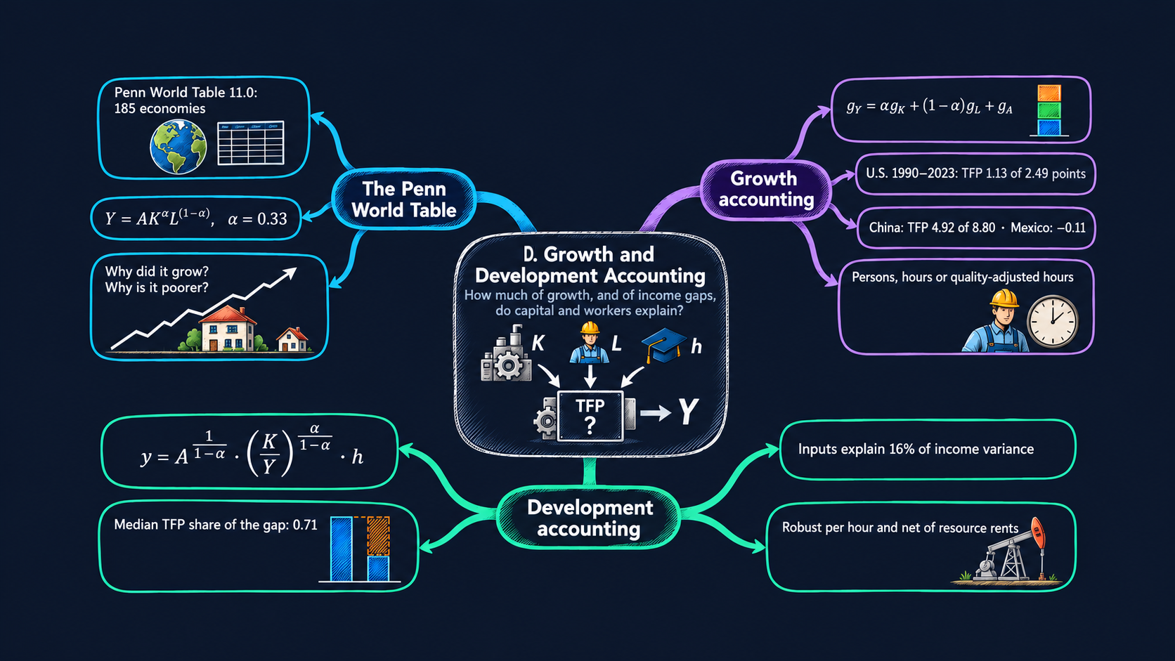
Two simple questions sit behind much of growth economics. Why did an economy grow as fast as it did? And why is one economy so much richer than another? Growth accounting answers the first question, and development accounting answers the second. Both split output into a part explained by measured inputs (physical capital, workers, hours, schooling) and a part that is left over, total factor productivity (TFP). This appendix applies both methods to the Penn World Table, for any economies you choose. By the end of it you will be able to:
- explain what the Penn World Table is, find the variables that the two methods need, and load them in Python, both from the official file and from the book’s prepared file;
- derive the growth accounting equation from a Cobb–Douglas production function, and compute the contributions of capital, labour and TFP to GDP growth for every year since 1990;
- derive the development accounting equation in its capital–output form, and split each economy’s income gap with the United States into TFP, physical capital and human capital;
- measure how much of the differences in income across countries the inputs can explain, with the “success” measure of development accounting;
- test how the answers change with the capital share, the measure of labour, country labour shares and natural-resource rents;
- write short pandas functions (
groupby,pct_change,merge,melt) and draw interactive Plotly charts that update when you choose other countries.
The appendix builds on the production model of Chapter 4, which does a first development accounting exercise with physical capital only, and on the growth accounting of Chapter 6, which uses U.S. data. The growth rules it uses are reviewed in Appendix C.5.
A map of the appendix
| Section | What you do | Builds on |
|---|---|---|
| D.1 | Two questions, two methods | Chapters 4 and 6 |
| D.2 | Set up, and choose your countries | Appendix A |
| D.3 | Meet the Penn World Table and load it | Chapter 3 |
| D.4 | Derive the growth accounting equation | Chapter 6, Appendix C.5 |
| D.5 | Growth accounting for one economy, step by step | — |
| D.6 | Growth accounting for your countries | — |
| D.7 | Averages over periods and decades | — |
| D.8 | Derive the development accounting equation | Chapter 4 |
| D.9 | Development accounting for your countries | — |
| D.10 | How much do inputs explain? | — |
| D.11 | Robustness: hours, labour shares, natural resources | — |
| D.12 | Go further | — |
The growth accounting of Sections D.4 to D.7 follows the method of the Growth Atlas, a study companion built on Penn World Table 11.0. The development accounting of Sections D.8 to D.11 follows the code of Julieta Caunedo’s STEG lecture on income accounting, which we translate from Stata to Python.
D.1 Two questions, two methods
Both methods start from the same production function, the one of Chapters 4 to 6:
\[ Y = A K^{\alpha} L^{1-\alpha}, \qquad 0 < \alpha < 1. \tag{1} \]
Output \(Y\) is made with physical capital \(K\) and labour \(L\), and \(A\) is total factor productivity: how efficiently the economy turns its inputs into output. The exponent \(\alpha\) is the capital share. We can measure \(Y\), \(K\) and \(L\) in national data, but not \(A\). Both methods therefore find \(A\) the same way: as the part of output that the measured inputs do not explain, the residual.
| Growth accounting | Development accounting | |
|---|---|---|
| Question | Why did this economy grow? | Why is this economy poorer than the United States? |
| Compares | one economy with itself, year after year | many economies with each other, in one year |
| Works with | growth rates of total GDP, capital and labour | levels of output per worker, capital and schooling |
| Main result | contributions of capital, labour and TFP to GDP growth, in percentage points | the share of the income gap due to TFP, physical capital and human capital |
| Sections | D.4 to D.7 | D.8 to D.11 |
Both methods are accounting, not explanation. They tell us where growth and income differences appear in equation (1), not why an economy invested more, schooled its workers longer, or used its inputs more efficiently. The models of Chapters 5 and 6 answer those questions.
D.2 Setup
The setup cell loads the libraries, sets the look of the charts and the address of the data files. It is the same as in the chapters.
Show the helper code
# @title Helper for the website versions (run this cell; you do not need to read it)
def slider_figure(make_figure, name, values, start, label=None):
    """Precompute make_figure(name=value) for every value and join the results with one slider.

    The website cannot run Python, so each interactive figure also gets this precomputed version.
    """
    figures = [make_figure(**{name: v}) for v in values]
    first = values.index(start)
    fig = go.Figure(layout=figures[first].layout)
    owner = []                                  # which precomputed figure each trace comes from
    for i, f in enumerate(figures):
        for trace in f.data:
            trace.visible = (i == first)
            fig.add_trace(trace)
            owner.append(i)
    steps = []
    for i, f in enumerate(figures):
        layout = {"title": f.layout.title.to_plotly_json(),
                  "annotations": [a.to_plotly_json() for a in f.layout.annotations],
                  "shapes": [s.to_plotly_json() for s in f.layout.shapes]}
        visible = [o == i for o in owner]
        steps.append(dict(method="update", label=str(values[i]), args=[{"visible": visible}, layout]))
    fig.update_layout(sliders=[dict(active=first, steps=steps, pad=dict(t=60),
                                    currentvalue=dict(prefix=(label or name) + " = "))])
    return fig
Choose your countries
Every chart of this appendix is drawn for a list of economies that you choose. Economies are named by their three-letter ISO code: USA for the United States, MEX for Mexico, CHN for China, IND for India, KOR for South Korea and NGA for Nigeria. To use other economies, change the list below and choose Runtime → Run all again. Section D.3 prints the codes of all 185 economies. In Colab, each chart also has a menu where you can pick economies with the mouse (hold Ctrl, or ⌘ on a Mac, to pick several).
COUNTRIES = ["USA", "MEX", "CHN", "IND", "KOR", "NGA"]   # your economies: change them!
ALPHA = 0.33                                             # the capital share, alpha
START, END = 1990, 2023                                  # the years of the growth accounting
Python note. Names in capital letters, such as
COUNTRIESorALPHA, are constants: values we set once at the top and use everywhere below. Changing them in one place changes the whole analysis.
D.3 The Penn World Table
The Penn World Table (PWT) is a database of national accounts for 185 economies since 1950, built at the Groningen Growth and Development Centre of the University of Groningen (Feenstra, Inklaar and Timmer 2015). It is the standard source for growth and development accounting, for two reasons:
- it makes output comparable across countries: GDP is converted with purchasing power parities (PPPs), so a dollar buys the same basket of goods everywhere, as Chapter 3 explains;
- it provides the inputs of the production function: capital stocks built from past investment, the number of workers, their hours, and an index of their schooling.
We use version 11.0, released in 2025, which covers 1950 to 2023 with prices of 2021. These are the variables we need:
| Variable | What it measures | Unit | Used in |
|---|---|---|---|
rgdpna |
real GDP at constant national prices | million 2021 US$ | growth accounting |
rnna |
capital stock at constant national prices | million 2021 US$ | growth accounting |
emp |
persons engaged (workers) | millions | both |
avh |
average hours worked per worker in a year | hours | both |
hc |
human capital index, from years of schooling and the return to schooling | index | both |
rgdpo |
real GDP at chained PPPs, output side | million 2021 US$ | development accounting |
cgdpo |
GDP at current PPPs, output side | million 2021 US$ | development accounting |
cn |
capital stock at current PPPs | million 2021 US$ | development accounting |
labsh |
share of labour income in GDP | share | Section D.11 |
Why two kinds of GDP? PWT recommends the national-price series (rgdpna, rnna) to compare growth rates over time within one economy, and the PPP series (rgdpo, cgdpo, cn) to compare levels across economies in one year. Growth accounting needs the first kind, development accounting the second.
Download the official file
The official data are a Stata file, pwt110.dta (about 4 MB), on the DataverseNL repository. pandas reads it straight from the web with pd.read_stata. The cell below downloads it, keeps the economies and years of this appendix, and prints its size.
PWT_URL = "https://dataverse.nl/api/access/datafile/554030"   # pwt110.dta, doi:10.34894/FABVLR
try:
    official = pd.read_stata(PWT_URL)
    print("Official PWT 11.0:", official.shape[0], "rows and", official.shape[1], "columns")
    print("Years:", official["year"].min(), "to", official["year"].max())
except Exception as error:
    official = None
    print("The download did not work (", error, "). The rest of the notebook does not need it.")
Official PWT 11.0: 13690 rows and 51 columns
Years: 1950 to 2023Python note.
try:runs a block of code, andexceptcatches an error instead of stopping the notebook. We use it here because the download depends on an outside server.
The full file has 51 columns. To keep the notebook fast, the book’s data script (build_data.py) keeps the nine variables of the table above, from 1970 to 2023, and adds a World Bank region for each economy. Every other number is unchanged, except for rounding to five significant digits. We load this prepared file and check that it agrees with the official one.
pwt = pd.read_csv(DATA_URL + "pwt_accounting.csv")
print(pwt.shape[0], "rows,", pwt["iso3"].nunique(), "economies,", pwt["year"].min(), "to", pwt["year"].max())
pwt.head()
9403 rows, 185 economies, 1970 to 2023| iso3 | country | region | year | rgdpna | rnna | emp | avh | hc | rgdpo | cgdpo | cn | labsh | |
|---|---|---|---|---|---|---|---|---|---|---|---|---|---|
| 0 | ALB | Albania | Europe & Central Asia | 1970 | 10013.0 | 29073.0 | 0.73130 | NaN | 1.5588 | 7150.4 | 6781.4 | 22712.0 | 0.83077 |
| 1 | ALB | Albania | Europe & Central Asia | 1971 | 10414.0 | 30921.0 | 0.75461 | NaN | 1.5868 | 7428.8 | 7036.6 | 24194.0 | 0.83077 |
| 2 | ALB | Albania | Europe & Central Asia | 1972 | 10832.0 | 32855.0 | 0.77834 | NaN | 1.6153 | 7735.7 | 7308.4 | 25762.0 | 0.83077 |
| 3 | ALB | Albania | Europe & Central Asia | 1973 | 11267.0 | 34877.0 | 0.80254 | NaN | 1.6443 | 8046.3 | 7565.5 | 27382.0 | 0.83077 |
| 4 | ALB | Albania | Europe & Central Asia | 1974 | 11715.0 | 36984.0 | 0.82714 | NaN | 1.6738 | 8385.4 | 7934.8 | 29102.0 | 0.83077 |
# Check: the prepared file and the official file agree (up to the rounding)
if official is not None:
    check = pwt.merge(official[["countrycode", "year", "rgdpna"]],
                      left_on=["iso3", "year"], right_on=["countrycode", "year"], suffixes=("", "_official"))
    gap = (check["rgdpna"] / check["rgdpna_official"] - 1).abs().max()
    print(f"Largest relative difference in rgdpna: {gap:.1e}")
Largest relative difference in rgdpna: 4.9e-05The country codes and names of all economies are in the columns iso3 and country. We keep them in a dictionary, NAMES, which turns a code into a name, and print the codes so you can choose your countries.
NAMES = dict(zip(pwt["iso3"], pwt["country"]))
print(len(NAMES), "economies:")
print(", ".join(code + " " + name for code, name in sorted(NAMES.items())))
185 economies:
ABW Aruba, AGO Angola, AIA Anguilla, ALB Albania, ARE United Arab Emirates, ARG Argentina, ARM Armenia, ATG Antigua and Barbuda, AUS Australia, AUT Austria, AZE Azerbaijan, BDI Burundi, BEL Belgium, BEN Benin, BFA Burkina Faso, BGD Bangladesh, BGR Bulgaria, BHR Bahrain, BHS Bahamas, BIH Bosnia and Herzegovina, BLR Belarus, BLZ Belize, BMU Bermuda, BOL Bolivia (Plurinational State of), BRA Brazil, BRB Barbados, BRN Brunei Darussalam, BTN Bhutan, BWA Botswana, CAF Central African Republic, CAN Canada, CHE Switzerland, CHL Chile, CHN China, CIV Côte d'Ivoire, CMR Cameroon, COD D.R. of the Congo, COG Congo, COL Colombia, COM Comoros, CPV Cabo Verde, CRI Costa Rica, CUW Curaçao, CYM Cayman Islands, CYP Cyprus, CZE Czechia, DEU Germany, DJI Djibouti, DMA Dominica, DNK Denmark, DOM Dominican Republic, DZA Algeria, ECU Ecuador, EGY Egypt, ESP Spain, EST Estonia, ETH Ethiopia, FIN Finland, FJI Fiji, FRA France, GAB Gabon, GBR United Kingdom, GEO Georgia, GHA Ghana, GIN Guinea, GMB Gambia, GNB Guinea-Bissau, GNQ Equatorial Guinea, GRC Greece, GRD Grenada, GTM Guatemala, GUY Guyana, HKG China, Hong Kong SAR, HND Honduras, HRV Croatia, HTI Haiti, HUN Hungary, IDN Indonesia, IND India, IRL Ireland, IRN Iran (Islamic Republic of), IRQ Iraq, ISL Iceland, ISR Israel, ITA Italy, JAM Jamaica, JOR Jordan, JPN Japan, KAZ Kazakhstan, KEN Kenya, KGZ Kyrgyzstan, KHM Cambodia, KNA Saint Kitts and Nevis, KOR Republic of Korea, KWT Kuwait, LAO Lao People's DR, LBN Lebanon, LBR Liberia, LCA Saint Lucia, LKA Sri Lanka, LSO Lesotho, LTU Lithuania, LUX Luxembourg, LVA Latvia, MAC China, Macao SAR, MAR Morocco, MDA Republic of Moldova, MDG Madagascar, MDV Maldives, MEX Mexico, MKD North Macedonia, MLI Mali, MLT Malta, MMR Myanmar, MNE Montenegro, MNG Mongolia, MOZ Mozambique, MRT Mauritania, MSR Montserrat, MUS Mauritius, MWI Malawi, MYS Malaysia, NAM Namibia, NER Niger, NGA Nigeria, NIC Nicaragua, NLD Netherlands, NOR Norway, NPL Nepal, NZL New Zealand, OMN Oman, PAK Pakistan, PAN Panama, PER Peru, PHL Philippines, POL Poland, PRT Portugal, PRY Paraguay, PSE State of Palestine, QAT Qatar, ROU Romania, RUS Russian Federation, RWA Rwanda, SAU Saudi Arabia, SDN Sudan, SEN Senegal, SGP Singapore, SLE Sierra Leone, SLV El Salvador, SOM Somalia, SRB Serbia, SSD South Sudan, STP Sao Tome and Principe, SUR Suriname, SVK Slovakia, SVN Slovenia, SWE Sweden, SWZ Eswatini, SXM Sint Maarten (Dutch part), SYC Seychelles, SYR Syrian Arab Republic, TCA Turks and Caicos Islands, TCD Chad, TGO Togo, THA Thailand, TJK Tajikistan, TKM Turkmenistan, TTO Trinidad and Tobago, TUN Tunisia, TUR Türkiye, TWN Taiwan, TZA U.R. of Tanzania: Mainland, UGA Uganda, UKR Ukraine, URY Uruguay, USA United States, UZB Uzbekistan, VCT St. Vincent and the Grenadines, VEN Venezuela (Bolivarian Republic of), VGB British Virgin Islands, VNM Viet Nam, YEM Yemen, ZAF South Africa, ZMB Zambia, ZWE ZimbabweFig. 1: Which data exist, and when?
Goal. Before any analysis, look at the coverage of the data. Not every economy has every variable in every year, and the gaps decide which economies we can compare.
coverage = pwt.groupby("year")[["rgdpna", "rnna", "emp", "hc", "avh", "labsh"]].count().reset_index()
coverage = coverage.melt(id_vars="year", var_name="variable", value_name="economies")
fig = px.line(coverage, x="year", y="economies", color="variable",
              color_discrete_sequence=[BLUE, TEAL, GREEN, RUST, PURPLE, GRAY],
              labels={"year": "Year", "economies": "Economies with data", "variable": "Variable"},
              title="Hours worked (avh) are measured for far fewer economies than GDP or capital",
              range_y=[0, 190])
fig
Sources. Data: Penn World Table 11.0 (Feenstra, Inklaar and Timmer 2015). Prepared file: data/appD/pwt_accounting.csv (see the data notes). Chart: inspired by the discussion of the Penn World Table in Chapter 3 of Jones (2024), Macroeconomics, 6th ed.
Python note.
groupby("year")[...].count()counts the non-missing values of each column, year by year.meltturns the six count columns into two columns,variableandeconomies, the “long” shape that Plotly Express wants: one row per point, and one column that names the line.
What to notice.
- GDP, capital and the number of workers exist for about 180 economies since 2000.
- Human capital (
hc) is missing for about 40 economies, mostly small islands and oil states. - Hours worked (
avh) cover only about 50 economies before 1990, mostly rich ones, and 130 since 2010. This is why the Growth Atlas, and Sections D.5 to D.9, measure labour by persons engaged by default, with hours as an option.
Your turn. From which year does each of your countries have data on hours worked (avh)?
Show the answer
mine = pwt[pwt["iso3"].isin(COUNTRIES)].dropna(subset=["avh"])
print(mine.groupby("country")["year"].min())
dropna removes the years with no hours, and groupby(...).min() finds the first year left for each country. All six default countries have hours in 2023, but Nigeria’s start only in 2005. With labour measured in hours, its growth accounting therefore starts in 2006.
# Your turn: try it hereFig. 2: A first look at your countries
Goal. Compare output per worker in your countries over time. Output per worker is the quantity that development accounting explains in Section D.9.
We compute it as PPP output (rgdpo) divided by persons engaged (emp). Both are in millions, so the ratio is in dollars per worker. A ratio scale shows equal growth rates as equal slopes (Appendix C).
pwt["y_worker"] = pwt["rgdpo"] / pwt["emp"]      # output per worker, 2021 US$ at PPP

def country_picker(value):
    """A menu of all economies, by name, that returns their codes."""
    options = sorted((name, code) for code, name in NAMES.items())
    return SelectMultiple(options=options, value=tuple(value), rows=8, description="economies", style=WIDE)

PALETTE = [BLUE, RUST, GREEN, PURPLE, TEAL, "#d4a017", "#5aa0d8", "#0b4f47", "#c2185b", "#6d4c41",
           "#00897b", "#7cb342", "#5e35b1", "#f4511e", "#3949ab", GRAY]

def country_colors(codes):
    """One fixed colour per economy: COUNTRIES first, in order, then the next free colours."""
    colors = {}
    order = list(COUNTRIES)
    for code in codes:
        if code not in order:
            order.append(code)
    for i, code in enumerate(order):
        colors[NAMES[code]] = PALETTE[i % len(PALETTE)]
    return colors
Python note.
country_colorsreturns a dictionary from country names to colours. Passing it to Plotly Express ascolor_discrete_mapkeeps each economy’s colour when you add or remove others in the menu.
def output_figure(codes=tuple(COUNTRIES)):
    """Fig. 2: output per worker for the chosen economies, ratio scale."""
    chosen = pwt[pwt["iso3"].isin(codes)]
    fig = px.line(chosen, x="year", y="y_worker", color="country", log_y=True,
                  color_discrete_map=country_colors(codes),
                  range_x=[1970, 2023], range_y=[500, 400000],
                  labels={"year": "Year", "y_worker": "Output per worker (2021 US$ at PPP, ratio scale)",
                          "country": ""},
                  title=f"Output per worker since 1970: {len(codes)} economies")
    fig.update_yaxes(tickvals=[1000, 3000, 10000, 30000, 100000, 300000])
    return fig

output_figure()
interact(output_figure, codes=country_picker(COUNTRIES));Show the code of the website version
# @title Website version: the default countries, with a linear/ratio switch
fig = output_figure()
buttons = [dict(label="Ratio scale", method="relayout",
                args=[{"yaxis.type": "log", "yaxis.range": [np.log10(500), np.log10(400000)]}]),
           dict(label="Linear scale", method="relayout",
                args=[{"yaxis.type": "linear", "yaxis.range": [0, 200000], "yaxis.tickvals": None}])]
fig.update_layout(updatemenus=[dict(type="buttons", buttons=buttons, direction="right", x=0.01, y=0.98,
                                    xanchor="left", yanchor="top")])
fig
Sources. Data: Penn World Table 11.0 (Feenstra, Inklaar and Timmer 2015), output-side real GDP at chained PPPs (rgdpo) divided by persons engaged (emp). Prepared file: data/appD/pwt_accounting.csv (see the data notes). Chart: inspired by the income comparisons in Chapter 3 of Jones (2024), Macroeconomics, 6th ed.
Python note.
country_pickerreturns aSelectMultiplemenu. Each option is a pair(name shown, value returned), so you see country names but the function receives codes.interactcallsoutput_figureagain every time you change the selection.
What to notice. Since 1970, China’s output per worker rose about 27-fold and Korea’s about 12-fold, while the U.S. level about doubled. Mexico’s output per worker was lower in 2023 than in 1980, and Nigeria’s is less than a tenth of the U.S. level. Large and lasting gaps like these are what development accounting tries to explain.
D.4 Growth accounting: the theory
Assumptions
- Output is produced with the Cobb–Douglas production function (1), \(Y_t = A_t K_t^{\alpha} L_t^{1-\alpha}\), in every year \(t\).
- The capital share \(\alpha\) is the same in every economy and every year. Following the Growth Atlas and Hall and Jones (1999), we use \(\alpha = 0.33\), about one third.
- Output \(Y_t\) is real GDP (
rgdpna), capital \(K_t\) is the real capital stock (rnna), and labour \(L_t\) is one of three measures: persons engaged (emp), total hours (emp×avh), or quality-adjusted hours (emp×avh×hc).
Deriving the equation
Take natural logs of equation (1). The log of a product is the sum of the logs, and the log of a power is the exponent times the log:
\[ \ln Y_t = \ln A_t + \alpha \ln K_t + (1-\alpha) \ln L_t . \]
The same equation holds a year earlier, at \(t-1\). Subtract the two:
\[ \ln Y_t - \ln Y_{t-1} = (\ln A_t - \ln A_{t-1}) + \alpha (\ln K_t - \ln K_{t-1}) + (1-\alpha)(\ln L_t - \ln L_{t-1}). \]
The change in the log of a variable is, approximately, its growth rate: \(\ln X_t - \ln X_{t-1} \approx \Delta X / X\). Writing \(g_X\) for the growth rate of \(X\) gives the growth accounting equation:
\[ g_Y = \underbrace{\alpha\, g_K}_{\text{capital}} + \underbrace{(1-\alpha)\, g_L}_{\text{labour}} + \underbrace{g_A}_{\text{TFP}} . \tag{2} \]
GDP growth is the sum of three contributions: the growth of capital weighted by its share \(\alpha\), the growth of labour weighted by its share \(1-\alpha\), and the growth of TFP.
The residual
We observe \(g_Y\), \(g_K\) and \(g_L\), but not \(g_A\). So we turn equation (2) around:
\[ g_A = g_Y - \alpha\, g_K - (1-\alpha)\, g_L . \tag{3} \]
TFP growth is whatever GDP growth the inputs cannot explain: the Solow residual. Because it is computed this way, the three contributions always add up to GDP growth exactly, even though equation (2) holds only approximately for growth rates. Like the Growth Atlas, we use simple yearly growth rates, \(g_X = 100 \times (X_t / X_{t-1} - 1)\), in percent, so each contribution is in percentage points.
Intuition. With \(\alpha = 0.33\), a 3 percent rise in the capital stock adds about 1 percentage point to GDP growth, and a 3 percent rise in labour adds about 2 points. Whatever growth is left is credited to TFP.
What the residual contains. Over long periods, TFP growth reflects new ideas (Chapter 6), better organization, and the movement of workers to more productive jobs. In a single year it also absorbs anything the inputs miss: changes in hours or skills when labour is counted in persons, how intensively machines are used in booms and recessions, commodity price swings, wars, and measurement error. Treat a large residual in a single year with care.
D.5 Growth accounting for one economy, step by step
Goal. Compute equation (3) by hand for the United States, one column at a time, and check that the contributions add up.
Step 1: the labour input. We start with persons engaged, the Growth Atlas default.
us = pwt[pwt["iso3"] == "USA"][["year", "rgdpna", "rnna", "emp"]].copy()
us["L"] = us["emp"]
us.tail(3)| year | rgdpna | rnna | emp | L | |
|---|---|---|---|---|---|
| 9061 | 2021 | 23681000.0 | 78159000.0 | 160.86 | 160.86 |
| 9062 | 2022 | 24276000.0 | 79490000.0 | 165.58 | 165.58 |
| 9063 | 2023 | 24977000.0 | 80823000.0 | 167.54 | 167.54 |
Step 2: growth rates. pct_change() computes \(X_t / X_{t-1} - 1\) for every row of a column.
us["g_Y"] = us["rgdpna"].pct_change() * 100
us["g_K"] = us["rnna"].pct_change() * 100
us["g_L"] = us["L"].pct_change() * 100
us[["year", "g_Y", "g_K", "g_L"]].tail(3).round(2)| year | g_Y | g_K | g_L | |
|---|---|---|---|---|
| 9061 | 2021 | 6.05 | 1.79 | 3.82 |
| 9062 | 2022 | 2.51 | 1.70 | 2.93 |
| 9063 | 2023 | 2.89 | 1.68 | 1.18 |
Step 3: the contributions, equations (2) and (3).
us["capital"] = ALPHA * us["g_K"]
us["labour"] = (1 - ALPHA) * us["g_L"]
us["tfp"] = us["g_Y"] - us["capital"] - us["labour"]
us = us[(us["year"] >= START) & (us["year"] <= END)]
us[["year", "g_Y", "capital", "labour", "tfp"]].tail(4).round(2)| year | g_Y | capital | labour | tfp | |
|---|---|---|---|---|---|
| 9060 | 2020 | -2.16 | 0.53 | -3.67 | 0.97 |
| 9061 | 2021 | 6.05 | 0.59 | 2.56 | 2.90 |
| 9062 | 2022 | 2.51 | 0.56 | 1.97 | -0.02 |
| 9063 | 2023 | 2.89 | 0.55 | 0.79 | 1.54 |
Step 4: check. The three contributions must add up to GDP growth in every year.
total = us["capital"] + us["labour"] + us["tfp"]
print("Largest gap between the sum and GDP growth:", (total - us["g_Y"]).abs().max())
print(f"Averages {START}-{END}: GDP {us['g_Y'].mean():.2f}%, capital {us['capital'].mean():.2f}, "
      f"labour {us['labour'].mean():.2f}, TFP {us['tfp'].mean():.2f} percentage points")
Largest gap between the sum and GDP growth: 4.440892098500626e-16
Averages 1990-2023: GDP 2.49%, capital 0.73, labour 0.63, TFP 1.13 percentage pointsThese numbers match the Growth Atlas, which publishes the same decomposition. For example, the Atlas reports U.S. GDP growth of 2.89 percent in 2023, with contributions of 0.55 (capital), 0.79 (labour) and 1.54 (TFP) percentage points.
A function for any economy and any labour measure
Steps 1 to 3 become one function. It works on many economies at once: groupby("iso3") makes pct_change compute growth rates within each economy, so the first year of one economy is never compared with the last year of another.
LABOUR = {"persons": "Persons engaged", "hours": "Total hours", "quality": "Quality-adjusted hours"}
LABOUR_MENU = [("Persons engaged", "persons"), ("Total hours", "hours"), ("Quality-adjusted hours", "quality")]

def growth_accounting(alpha=ALPHA, labour="persons"):
    """Equations (2) and (3) for every economy: contributions to GDP growth, in percentage points."""
    d = pwt.sort_values(["iso3", "year"]).copy()
    d["L"] = d["emp"]
    if labour in ("hours", "quality"):
        d["L"] = d["L"] * d["avh"]
    if labour == "quality":
        d["L"] = d["L"] * d["hc"]
    growth = d.groupby("iso3")[["rgdpna", "rnna", "L"]].pct_change(fill_method=None) * 100
    d["gdp"] = growth["rgdpna"]
    d["capital"] = alpha * growth["rnna"]
    d["labour"] = (1 - alpha) * growth["L"]
    d["tfp"] = d["gdp"] - d["capital"] - d["labour"]
    d = d[(d["year"] >= START) & (d["year"] <= END)]
    return d[["iso3", "country", "year", "gdp", "capital", "labour", "tfp"]].dropna()

ga = growth_accounting()
print(ga["iso3"].nunique(), "economies,", len(ga), "economy-years")
ga[ga["iso3"].isin(COUNTRIES)].groupby("country")[["gdp", "capital", "labour", "tfp"]].mean().round(2)
180 economies, 5978 economy-years| gdp | capital | labour | tfp | |
|---|---|---|---|---|
| country | ||||
| China | 8.80 | 3.52 | 0.36 | 4.92 |
| India | 6.06 | 2.20 | 1.39 | 2.47 |
| Mexico | 2.29 | 0.83 | 1.57 | -0.11 |
| Nigeria | 4.25 | 0.42 | 2.18 | 1.65 |
| Republic of Korea | 4.89 | 2.12 | 0.95 | 1.82 |
| United States | 2.49 | 0.73 | 0.63 | 1.13 |
Python note.
pct_change(fill_method=None)leaves a growth rate missing when either year is missing, instead of filling the gap.dropna()then removes the rows with any missing value.
Fig. 3: The growth accounting of one economy
Goal. Draw the decomposition year by year: stacked bars for the three contributions, and a line for GDP growth. The bars of each year add up to the line.
PARTS = [("capital", "Capital, αg_K", BLUE), ("labour", "Labour, (1−α)g_L", GREEN), ("tfp", "TFP, g_A", RUST)]

def add_decomposition(fig, d, row=None, col=None, legend=True):
    """Add the three contribution bars and the GDP growth line of one economy to a figure."""
    for column, label, color in PARTS:
        fig.add_trace(go.Bar(x=d["year"], y=d[column], name=label, marker_color=color,
                             legendgroup=column, showlegend=legend), row=row, col=col)
    fig.add_trace(go.Scatter(x=d["year"], y=d["gdp"], mode="lines+markers", name="GDP growth, g_Y",
                             line=dict(color="black", width=2), marker=dict(size=4),
                             legendgroup="gdp", showlegend=legend), row=row, col=col)
    return fig

def decomposition_figure(code="USA", alpha=ALPHA, labour="persons"):
    """Fig. 3: contributions to GDP growth in one economy, equation (2)."""
    d = growth_accounting(alpha, labour)
    d = d[d["iso3"] == code]
    fig = add_decomposition(go.Figure(), d)
    fig.update_layout(barmode="relative", title=f"{NAMES[code]}: where GDP growth came from, {START}-{END}",
                      xaxis_title="Year", yaxis_title="Percentage points", legend=dict(orientation="h", y=-0.15))
    return fig

decomposition_figure()
Sources. Data: Penn World Table 11.0 (Feenstra, Inklaar and Timmer 2015), rgdpna, rnna and emp. Prepared file: data/appD/pwt_accounting.csv (see the data notes). Method: the Growth Atlas. Chart: inspired by the growth accounting of Chapter 6 in Jones (2024), Macroeconomics, 6th ed.
Python note.
barmode="relative"stacks positive bars upwards and negative bars downwards from zero, so a year with a negative contribution still reads correctly.legendgroupties the bars of one kind together, which matters when the same legend serves several panels (Fig. 4).
What to notice.
- In 2020 the pandemic cut U.S. employment, so the labour contribution fell to about −3.7 percentage points, while TFP rose. Workers who kept their jobs were, on average, more productive, and output per worker held up: a classic composition effect that the residual absorbs.
- TFP contributions swing much more from year to year than capital contributions, because the capital stock changes slowly while output moves with the business cycle.
D.6 Growth accounting for your countries
Fig. 4: Contributions to GDP growth, economy by economy
Goal. Compare the growth accounting of several economies side by side, and test how it changes with the capital share \(\alpha\) and the measure of labour.
Some economies lack hours or human capital in some years. A small helper writes their codes under the title, so a missing panel is never a mystery.
def no_data_note(codes, d):
    """A small second title line naming the chosen economies that have no data in d."""
    missing = []
    for code in codes:
        if code not in set(d["iso3"]):
            missing.append(code)
    if len(missing) == 0:
        return ""
    return "<br><sup>No data: " + ", ".join(missing) + "</sup>"
def growth_panels(codes=tuple(COUNTRIES), alpha=ALPHA, labour="persons"):
"""Fig. 4: one growth accounting panel per chosen economy, equation (2)."""
d = growth_accounting(alpha, labour)
codes = list(codes)[:9] # at most nine panels
if len(codes) == 0:
codes = ["USA"] # nothing chosen: show the United States
rows = (len(codes) + 2) // 3
titles = []
for code in codes:
titles.append(NAMES[code][:28])
fig = make_subplots(rows=rows, cols=3, shared_yaxes=True, vertical_spacing=0.12, subplot_titles=titles)
for i, code in enumerate(codes):
add_decomposition(fig, d[d["iso3"] == code], row=i // 3 + 1, col=i % 3 + 1, legend=(i == 0))
note = no_data_note(codes, d)
fig.update_layout(barmode="relative", height=300 + 260 * rows, legend=dict(orientation="h", y=-0.08),
title=f"Contributions to GDP growth, α = {alpha:.2f}, labour = {LABOUR[labour]}{note}")
shown = d[d["iso3"].isin(codes)][["gdp", "capital", "labour", "tfp"]]
if shown.abs().max().max() < 20: # one fixed scale, unless a year is far outside it
fig.update_yaxes(range=[-20, 20])
return fig
growth_panels()interact(growth_panels, codes=country_picker(COUNTRIES),
alpha=FloatSlider(value=ALPHA, min=0.2, max=0.5, step=0.01, description="capital share α", style=WIDE),
labour=Dropdown(options=LABOUR_MENU, value="persons", description="labour measure", style=WIDE));Show the code of the website version
# @title Website version: one economy at a time, chosen from a menu
complete = ga.groupby("iso3")["year"].count()
menu_codes = sorted(complete[complete == END - START + 1].index, key=NAMES.get)
fig = go.Figure()
for code in menu_codes:
    add_decomposition(fig, ga[ga["iso3"] == code].round(2), legend=(code == menu_codes[0]))
buttons = []
for i, code in enumerate(menu_codes):
    visible = [j // 4 == i for j in range(4 * len(menu_codes))]
    buttons.append(dict(label=NAMES[code][:30], method="update",
                        args=[{"visible": visible}, {"title": f"{NAMES[code]}: contributions to GDP growth"}]))
for j, trace in enumerate(fig.data):
    trace.visible = (j // 4 == menu_codes.index("USA"))
    trace.showlegend = trace.visible
fig.update_layout(barmode="relative", title="United States: contributions to GDP growth", height=560,
                  xaxis=dict(title="Year", range=[1989.5, 2023.5]), yaxis_title="Percentage points",
                  legend=dict(orientation="h", y=-0.15), margin=dict(t=120),
                  updatemenus=[dict(buttons=buttons, active=menu_codes.index("USA"), x=1, y=1.06,
                                    xanchor="right", yanchor="bottom")])
fig
Sources. Data: Penn World Table 11.0 (Feenstra, Inklaar and Timmer 2015), rgdpna, rnna, emp, avh and hc. Prepared file: data/appD/pwt_accounting.csv (see the data notes). Method: the Growth Atlas. Chart: inspired by the growth accounting of Chapter 6 in Jones (2024), Macroeconomics, 6th ed.
On the website, choose an economy from the menu above the chart. The menu lists the economies with complete data from 1990 to 2023, with labour measured in persons engaged and \(\alpha = 0.33\). In Colab, the controls above also let you change \(\alpha\) and the labour measure, and compare up to nine economies.
What to notice.
- China grew fastest, and both capital and TFP contributed a lot. Its capital contribution stayed above 2 percentage points in almost every year.
- India and Nigeria had large labour contributions: their working-age populations grew fast.
- Mexico’s growth came almost entirely from adding capital and workers; its average TFP contribution was slightly negative.
- Raising \(\alpha\) moves growth from labour to capital in economies whose capital grew faster than labour (China, Korea), and lowers their TFP. Switching from persons to hours lowers the labour contribution where hours per worker fell (Korea), and moves that growth into TFP.
Your turn. Add Vietnam (VNM) and Indonesia (IDN) to the chart. Which of the two had the larger average TFP contribution from 1990 to 2023?
Show the answer
two = ga[ga["iso3"].isin(["VNM", "IDN"])]
print(two.groupby("country")[["gdp", "capital", "labour", "tfp"]].mean().round(2))
Vietnam grew faster than Indonesia, with larger contributions from capital and from TFP. In Colab you can also pick both names in the menu of Fig. 4.
# Your turn: try it hereD.7 Averages over periods and decades
Yearly numbers are noisy. Over longer periods, business-cycle swings cancel out and the residual reflects long-run productivity growth more closely.
Fig. 5: Average contributions over a period
Goal. Compare average contributions across your economies over a period you choose.
def period_averages(codes=tuple(COUNTRIES), start=START, end=END, alpha=ALPHA, labour="persons"):
    """Average contributions to GDP growth over start-end, one row per economy."""
    d = growth_accounting(alpha, labour)
    d = d[d["iso3"].isin(codes) & (d["year"] >= start) & (d["year"] <= end)]
    return d.groupby("country")[["gdp", "capital", "labour", "tfp"]].mean().sort_values("gdp")

def average_figure(codes=tuple(COUNTRIES), start=START, end=END, alpha=ALPHA, labour="persons"):
    """Fig. 5: stacked average contributions, with average GDP growth as a diamond."""
    avg = period_averages(codes, start, end, alpha, labour).reset_index()
    avg["gdp"] = avg["gdp"].round(4)
    fig = go.Figure()
    for column, label, color in PARTS:
        fig.add_trace(go.Bar(x=avg["country"], y=avg[column], name=label, marker_color=color))
    fig.add_trace(go.Scatter(x=avg["country"], y=avg["gdp"], mode="markers", name="GDP growth, g_Y",
                             marker=dict(color="black", symbol="diamond", size=12)))
    fig.update_layout(barmode="relative", title=f"Average contributions to GDP growth, {start}-{end}",
                      yaxis_title="Percentage points a year")
    parts = avg[["capital", "labour", "tfp"]]
    if parts.clip(lower=0).sum(axis=1).max() < 12 and parts.clip(upper=0).sum(axis=1).min() > -4:
        fig.update_yaxes(range=[-4, 12])            # one fixed scale, so periods are easy to compare
    return fig

average_figure()
interact(average_figure, codes=country_picker(COUNTRIES),
start=IntSlider(value=START, min=1971, max=2022, description="from", style=WIDE),
end=IntSlider(value=END, min=1972, max=2023, description="to", style=WIDE),
alpha=FloatSlider(value=ALPHA, min=0.2, max=0.5, step=0.01, description="capital share α", style=WIDE),
labour=Dropdown(options=LABOUR_MENU, value="persons", description="labour measure", style=WIDE));Show the code of the website version
# @title Website version: the default countries, with a slider over periods
PERIODS = {"1990-1999": (1990, 1999), "2000-2009": (2000, 2009), "2010-2019": (2010, 2019),
           "2020-2023": (2020, 2023), "1990-2023": (1990, 2023)}

def period_figure(period="1990-2023"):
    """Fig. 5 for one of the periods above."""
    return average_figure(start=PERIODS[period][0], end=PERIODS[period][1])

fig = slider_figure(period_figure, "period", ["1990-1999", "2000-2009", "2010-2019", "2020-2023", "1990-2023"],
                    start="1990-2023", label="period")
fig.update_layout(height=600)
fig
Sources. Data: Penn World Table 11.0 (Feenstra, Inklaar and Timmer 2015). Prepared file: data/appD/pwt_accounting.csv (see the data notes). Method: the Growth Atlas. Chart: inspired by the growth accounting of Chapter 6 in Jones (2024), Macroeconomics, 6th ed.
What to notice. Over 1990–2023, TFP accounts for more than half of China’s growth, close to half of the growth of the United States, and nothing in Mexico. Move the slider through the decades: Korea’s TFP contribution shrinks as the economy matures, and the period 2020–2023 is dominated by the pandemic.
The growth accounting by decade
A table by decade shows the same story in numbers. year // 10 * 10 turns each year into its decade (2017 → 2010).
decades = ga[ga["iso3"].isin(COUNTRIES)].copy()
decades["decade"] = decades["year"] // 10 * 10
table = decades.groupby(["country", "decade"])[["gdp", "capital", "labour", "tfp"]].mean().round(2)
table| gdp | capital | labour | tfp | ||
|---|---|---|---|---|---|
| country | decade | ||||
| China | 1990 | 9.99 | 3.26 | 0.90 | 5.84 |
| 2000 | 10.35 | 3.99 | 0.46 | 5.91 | |
| 2010 | 7.68 | 3.70 | -0.01 | 3.99 | |
| 2020 | 4.72 | 2.56 | -0.32 | 2.48 | |
| India | 1990 | 5.77 | 1.74 | 1.19 | 2.83 |
| 2000 | 6.28 | 2.49 | 1.00 | 2.80 | |
| 2010 | 6.64 | 2.42 | 1.05 | 3.17 | |
| 2020 | 4.76 | 2.01 | 3.75 | -1.00 | |
| Mexico | 1990 | 3.71 | 0.98 | 2.01 | 0.71 |
| 2000 | 1.27 | 0.87 | 1.46 | -1.06 | |
| 2010 | 2.33 | 0.77 | 1.32 | 0.23 | |
| 2020 | 1.17 | 0.45 | 1.37 | -0.64 | |
| Nigeria | 1990 | 2.31 | 0.43 | 1.24 | 0.64 |
| 2000 | 7.68 | 0.31 | 2.47 | 4.89 | |
| 2010 | 3.65 | 0.48 | 2.75 | 0.43 | |
| 2020 | 1.99 | 0.53 | 2.32 | -0.86 | |
| Republic of Korea | 1990 | 7.43 | 3.55 | 1.00 | 2.88 |
| 2000 | 4.92 | 1.91 | 1.01 | 2.00 | |
| 2010 | 3.47 | 1.31 | 0.92 | 1.25 | |
| 2020 | 2.01 | 1.08 | 0.80 | 0.13 | |
| United States | 1990 | 3.23 | 0.88 | 0.76 | 1.58 |
| 2000 | 1.92 | 0.86 | 0.25 | 0.81 | |
| 2010 | 2.40 | 0.52 | 0.96 | 0.92 | |
| 2020 | 2.32 | 0.56 | 0.41 | 1.35 |
Python note.
//is integer division:2017 // 10is201, and201 * 10is2010. Grouping by two columns gives a table with one row per country and decade.
Your turn. In which decade was China’s TFP contribution largest, and how large was it?
Show the answer
china = table.loc["China"]
print(china)
print("Largest TFP contribution:", china["tfp"].idxmax(), china["tfp"].max())
table.loc["China"] keeps the rows of China; idxmax() returns the decade where the TFP column is largest.
# Your turn: try it hereD.8 Development accounting: the theory
Growth accounting compares an economy with its own past. Development accounting compares economies with each other in one year. Chapter 4 did a first version: with output per person \(y = \bar{A} k^{1/3}\), it found that differences in capital per person explain little of the income gap between rich and poor economies, and TFP explains most of it. We now add human capital, and write the equation in a form that avoids crediting capital for what TFP achieved.
Assumptions
- Output is produced with physical capital \(K\) and human capital \(H = hL\): \(L\) workers, each with \(h\) units of skills from schooling (PWT’s
hcindex), \[Y = A K^{\alpha} (hL)^{1-\alpha} . \tag{4}\] - The capital share is \(\alpha = 0.33\) in every economy, as in Hall and Jones (1999) and Caunedo’s code.
- Output and capital are measured at PPPs, so they are comparable across economies: output per worker \(y = Y/L\) is
rgdpo / emp, and the capital–output ratio \(K/Y\) iscn / cgdpo.
Deriving the equation
Divide equation (4) by \(L\). With \(k = K/L\), output per worker is
\[ y = A k^{\alpha} h^{1-\alpha} . \]
This is the form of Chapter 4, with schooling added. But \(k\) is not independent of \(A\): an economy with a higher TFP produces more, saves more and builds a larger capital stock (Chapter 5). Part of its high \(k\) is therefore caused by TFP. To avoid crediting capital for it, write capital per worker as the capital–output ratio times output per worker, \(k = (K/Y)\, y\):
\[ y = A \left(\frac{K}{Y}\right)^{\alpha} y^{\alpha} h^{1-\alpha} . \]
Divide both sides by \(y^{\alpha}\), so the left side becomes \(y^{1-\alpha}\):
\[ y^{1-\alpha} = A \left(\frac{K}{Y}\right)^{\alpha} h^{1-\alpha} . \]
Raise both sides to the power \(1/(1-\alpha)\):
\[ y = \underbrace{A^{\frac{1}{1-\alpha}}}_{\text{TFP term}} \;\times\; \underbrace{\left(\frac{K}{Y}\right)^{\frac{\alpha}{1-\alpha}}}_{\text{capital term}} \;\times\; \underbrace{h}_{\text{human capital}} . \tag{5} \]
Output per worker is the product of three terms. In the Solow model the capital–output ratio is \(s/(n+\bar{d})\) in steady state, which does not depend on \(A\), so the capital term measures the part of capital that is not driven by TFP. Hall and Jones (1999) and Caselli (2005) discuss this choice.
The residual and the comparison with the United States
As in growth accounting, the TFP term is the residual: what is left of \(y\) after the measured inputs,
\[ A^{\frac{1}{1-\alpha}} = \frac{y}{(K/Y)^{\alpha/(1-\alpha)}\; h} . \tag{6} \]
Divide equation (5) for economy \(i\) by the same equation for the United States. Each term becomes a ratio, and a value of 0.5 means “half the U.S. level”:
\[ \frac{y_i}{y_{US}} = \frac{A_i^{1/(1-\alpha)}}{A_{US}^{1/(1-\alpha)}} \times \frac{(K/Y)_i^{\alpha/(1-\alpha)}}{(K/Y)_{US}^{\alpha/(1-\alpha)}} \times \frac{h_i}{h_{US}} . \tag{7} \]
Splitting the gap
Turn each ratio upside down to get the gap factors: \(T_i\) for TFP, \(K_i\) for the capital term and \(H_i\) for human capital, each equal to the U.S. level divided by economy \(i\)’s level. The income gap is their product, \(y_{US}/y_i = T_i \times K_i \times H_i\). Caunedo’s code compares the TFP gap with the gap that the two inputs create together, \(K_i \times H_i\), and splits the rest between the two inputs in proportion to their gap factors:
\[ s^{TFP}_i = \frac{T_i}{T_i + K_i H_i}, \qquad s^{K}_i = \frac{K_i}{K_i + H_i}\,(1 - s^{TFP}_i), \qquad s^{H}_i = \frac{H_i}{K_i + H_i}\,(1 - s^{TFP}_i) . \tag{8} \]
The three shares add up to one. If TFP and the inputs open gaps of the same size (\(T_i = K_i H_i\)), the TFP share is one half; if the TFP gap is three times the input gap, it is three quarters.
Intuition. Development accounting asks: if this economy had U.S. levels of capital (relative to output) and of schooling, how much richer would it be? The TFP term answers what is left: how much it would still lag behind.
D.9 Development accounting for your countries
Goal. Compute equations (5) to (8) for every economy in one year, with labour measured per worker (the default) or per hour.
The function keeps one year, computes the three terms of equation (5), divides by the U.S. values, and adds the shares of equation (8). It drops Venezuela, whose PWT output after 2017 is not plausible (hyperinflation broke its price data), as in the chapters.
def dev_levels(year=2023, per="worker", alpha=ALPHA):
    """Equations (5) and (6): output per worker, the capital term, human capital and TFP, in one year."""
    d = pwt[(pwt["year"] == year) & (pwt["iso3"] != "VEN")].copy()
    d["workers"] = d["emp"]
    if per == "hour":
        d["workers"] = d["emp"] * d["avh"]          # output per hour instead of per worker
    d["y"] = d["rgdpo"] / d["workers"]
    d["ky"] = (d["cn"] / d["cgdpo"]) ** (alpha / (1 - alpha))
    d["h"] = d["hc"]
    d["tfp"] = d["y"] / (d["ky"] * d["h"])
    return d.dropna(subset=["y", "ky", "h", "tfp"])
def relative_to_us(d):
"""Equations (7) and (8): each term relative to the United States, and the shares of the gap."""
d = d.copy()
us = d[d["iso3"] == "USA"].iloc[0]
for col in ["y", "ky", "h", "tfp"]:
d[col + "_rel"] = d[col] / us[col]
T, K, H = 1 / d["tfp_rel"], 1 / d["ky_rel"], 1 / d["h_rel"]
d["share_tfp"] = T / (T + K * H)
d["share_k"] = K / (K + H) * (1 - d["share_tfp"])
d["share_h"] = H / (K + H) * (1 - d["share_tfp"])
d.loc[d["iso3"] == "USA", ["share_tfp", "share_k", "share_h"]] = np.nan # no gap with itself
return d
def dev_accounting(year=2023, per="worker", alpha=ALPHA):
"""Development accounting in one year: levels, ratios to the United States and shares."""
return relative_to_us(dev_levels(year, per, alpha))
da = dev_accounting()
print(len(da), "economies in 2023")
mine = da[da["iso3"].isin(COUNTRIES)].set_index("country")
mine[["y_rel", "ky_rel", "h_rel", "tfp_rel", "share_tfp", "share_k", "share_h"]].round(3)143 economies in 2023| y_rel | ky_rel | h_rel | tfp_rel | share_tfp | share_k | share_h | |
|---|---|---|---|---|---|---|---|
| country | |||||||
| China | 0.276 | 1.306 | 0.718 | 0.294 | 0.761 | 0.085 | 0.154 |
| India | 0.129 | 1.115 | 0.596 | 0.193 | 0.775 | 0.079 | 0.147 |
| Mexico | 0.292 | 1.134 | 0.745 | 0.346 | 0.709 | 0.115 | 0.175 |
| Nigeria | 0.085 | 1.729 | 0.557 | 0.088 | 0.916 | 0.020 | 0.063 |
| Republic of Korea | 0.685 | 1.255 | 1.011 | 0.540 | 0.702 | 0.133 | 0.165 |
| United States | 1.000 | 1.000 | 1.000 | 1.000 | NaN | NaN | NaN |
Check. Equation (7) says the three ratios multiply to the output ratio, and equation (8) says the three shares add up to one.
product = da["tfp_rel"] * da["ky_rel"] * da["h_rel"]
print("Largest error in equation (7):", (product - da["y_rel"]).abs().max())
print("Largest error in the shares:", (da["share_tfp"] + da["share_k"] + da["share_h"] - 1).abs().max())
Largest error in equation (7): 2.220446049250313e-16
Largest error in the shares: 1.1102230246251565e-16Fig. 6: The three terms, relative to the United States
Goal. See which term is furthest from the U.S. level in each of your economies.
TERMS = [("y_rel", "Output per worker, y", "black"), ("ky_rel", "Capital term, (K/Y)^(α/(1−α))", BLUE),
         ("h_rel", "Human capital, h", TEAL), ("tfp_rel", "TFP term, A^(1/(1−α))", RUST)]

def terms_figure(codes=tuple(COUNTRIES), year=2023, per="worker"):
    """Fig. 6: the terms of equation (7) for the chosen economies, United States = 1."""
    d = dev_accounting(year, per)
    d = d[d["iso3"].isin(codes)].sort_values("y_rel")
    fig = go.Figure()
    for column, label, color in TERMS:
        fig.add_trace(go.Bar(x=d["country"].str[:22], y=d[column].round(3), name=label, marker_color=color))
    fig.add_hline(y=1, line_dash="dash", line_color=GRAY)
    note = no_data_note(codes, d)
    fig.update_layout(barmode="group", title=f"Development accounting per {per}, {year} (United States = 1){note}",
                      yaxis_title="Ratio to the United States", legend=dict(orientation="h", y=-0.15))
    if d[["y_rel", "ky_rel", "h_rel", "tfp_rel"]].max().max() < 2.4:
        fig.update_yaxes(range=[0, 2.4])            # one fixed scale, unless an economy is far above it
    return fig

terms_figure()
interact(terms_figure, codes=country_picker(COUNTRIES),
year=IntSlider(value=2023, min=1970, max=2023, description="year", style=WIDE),
per=ToggleButtons(options=[("Per worker", "worker"), ("Per hour", "hour")], value="worker",
description="output", style=WIDE));Show the code of the website version
# @title Website version: the default countries, with a slider over years
fig = slider_figure(terms_figure, "year", [1990, 2000, 2010, 2023], start=2023, label="year")
fig.update_layout(height=620)
fig.layout.sliders[0].pad.t = 140                  # leave room for the legend under the plot
fig
Sources. Data: Penn World Table 11.0 (Feenstra, Inklaar and Timmer 2015), rgdpo, cgdpo, cn, emp, avh and hc. Prepared file: data/appD/pwt_accounting.csv (see the data notes). Method: Caunedo, STEG Lecture 2. Chart: inspired by the development accounting of Chapter 4 in Jones (2024), Macroeconomics, 6th ed.
What to notice.
- The capital term is close to 1, or above it, in every one of the default economies: poorer economies do not have lower capital–output ratios. Capital per worker is low in Nigeria because output per worker is low, not the other way round.
- Human capital in India and Nigeria is about 55 to 60 percent of the U.S. level: schooling explains part of the gap.
- The TFP term is the furthest from 1. Nigeria’s is about 9 percent of the U.S. level, India’s about 19 percent. Most of the income gap is a TFP gap.
Fig. 7: How much of the gap is due to TFP?
Goal. Look at all economies at once: plot the TFP share of each economy’s gap, equation (8), against its output per worker.
def share_scatter(codes=tuple(COUNTRIES), year=2023):
    """Fig. 7: the TFP share of the income gap against output per worker, all economies."""
    d = dev_accounting(year).dropna(subset=["share_tfp"])
    d["group"] = np.where(d["iso3"].isin(codes), "Your economies", "Other economies")
    d["label"] = np.where(d["iso3"].isin(codes), d["iso3"], "")
    fig = px.scatter(d, x="y_rel", y="share_tfp", color="group", text="label", hover_name="country",
                     log_x=True, range_x=[0.008, 12], range_y=[0, 1.05],
                     color_discrete_map={"Your economies": RUST, "Other economies": BLUE},
                     labels={"y_rel": "Output per worker (United States = 1, ratio scale)",
                             "share_tfp": "Share of the gap due to TFP", "group": ""},
                     title=f"In {year}, the poorer the economy, the larger the share of its gap due to TFP")
    fig.update_traces(textposition="top center")
    fig.update_xaxes(tickvals=[0.01, 0.03, 0.1, 0.3, 1, 3, 10])
    return fig

share_scatter()
interact(share_scatter, codes=country_picker(COUNTRIES),
year=IntSlider(value=2023, min=1970, max=2023, description="year", style=WIDE));Show the code of the website version
# @title Website version: all years, with a play button
frames = []
for year in range(1990, 2024):
    d = dev_accounting(year).dropna(subset=["share_tfp"])
    frames.append(d[["iso3", "country", "year", "y_rel", "share_tfp"]])
panel = pd.concat(frames)
panel["group"] = np.where(panel["iso3"].isin(COUNTRIES), "Your economies", "Other economies")
panel["label"] = np.where(panel["iso3"].isin(COUNTRIES), panel["iso3"], "")
panel = panel.sort_values(["year", "group", "iso3"]).round(4)
fig = px.scatter(panel, x="y_rel", y="share_tfp", color="group", text="label", hover_name="country",
                 animation_frame="year", animation_group="iso3", log_x=True,
                 range_x=[0.008, 12], range_y=[0, 1.05],
                 color_discrete_map={"Your economies": RUST, "Other economies": BLUE},
                 labels={"y_rel": "Output per worker (United States = 1, ratio scale)",
                         "share_tfp": "Share of the gap due to TFP", "group": ""},
                 title="The share of the income gap due to TFP, 1990-2023 (press play)")
fig.update_traces(textposition="top center")
fig.update_xaxes(tickvals=[0.01, 0.03, 0.1, 0.3, 1, 3, 10])
fig.layout.sliders[0].active = len(fig.frames) - 1          # start on 2023
fig.update_traces(x=fig.frames[-1].data[0].x, y=fig.frames[-1].data[0].y, text=fig.frames[-1].data[0].text,
                  hovertext=fig.frames[-1].data[0].hovertext, selector=dict(name="Other economies"))
fig.update_traces(x=fig.frames[-1].data[1].x, y=fig.frames[-1].data[1].y, text=fig.frames[-1].data[1].text,
                  hovertext=fig.frames[-1].data[1].hovertext, selector=dict(name="Your economies"))
fig
Sources. Data: Penn World Table 11.0 (Feenstra, Inklaar and Timmer 2015). Prepared file: data/appD/pwt_accounting.csv (see the data notes). Method and chart: inspired by Caunedo, STEG Lecture 2, and by the development accounting of Chapter 4 in Jones (2024), Macroeconomics, 6th ed.
What to notice.
- In the 31 poorest economies, with less than a tenth of U.S. output per worker, TFP accounts for 70 to 90 percent of the gap in most cases (the median is about 80 percent).
- Economies richer than the United States (Ireland, Norway, Switzerland, Singapore, Qatar, Brunei) appear on the right of 1. Their “gaps” are negative, and the shares measure how much each term contributes to their lead.
- Press play on the website: the cloud drifts up over time. TFP explains a larger share of income gaps in 2023 than in 1990, as Fig. 8 shows more clearly.
Your turn. Compute the TFP share of the gap for Korea per worker and per hour in 2023. Why do they differ?
Show the answer
for per in ["worker", "hour"]:
    d = dev_accounting(2023, per)
    korea = d[d["iso3"] == "KOR"].iloc[0]
    print(per, round(korea["y_rel"], 3), round(korea["share_tfp"], 3))
Koreans work more hours a year than Americans, so Korea is further behind in output per hour than in output per worker. Its TFP gap, and the TFP share, are larger per hour.
# Your turn: try it hereD.10 How much do inputs explain?
Equation (8) gives a share for each economy. Two summary measures describe all economies together.
The success of factor-only models
Caselli (2005) asks a different question: if all economies had the same TFP, how much of the dispersion of income across economies would remain? Write \(y^{KH}_i = (K/Y)_i^{\alpha/(1-\alpha)} h_i\) for the part of output per worker explained by the inputs in equation (5). The success of this factor-only model is the ratio of the variances of the logs:
\[ \text{success} = \frac{\operatorname{var}\left[\ln y^{KH}\right]}{\operatorname{var}\left[\ln y\right]} . \tag{9} \]
A success of 1 means inputs explain all of the differences in income; a success of 0 means they explain none. Caunedo’s code also reports the success of each input on its own.
def success(d):
    """Equation (9): the share of the variance of log output per worker explained by the inputs."""
    var_y = np.log(d["y"]).var()
    return {"economies": len(d),
            "inputs": np.log(d["ky"] * d["h"]).var() / var_y,
            "physical capital": np.log(d["ky"]).var() / var_y,
            "human capital": np.log(d["h"]).var() / var_y}

result = success(dev_levels(2023))
for key, value in result.items():
    print(f"{key:>17}: {value:.3f}")
economies: 143.000
inputs: 0.157
physical capital: 0.053
human capital: 0.068What to notice. Inputs explain only about 16 percent of the variance of log output per worker across 143 economies in 2023. The other 84 percent is TFP.
This is lower than the success of about 0.3 to 0.4 that Caselli (2005) reports with the form of Chapter 4, \(y^{KH} = k^{\alpha} h^{1-\alpha}\). That form credits physical capital for the capital that TFP itself induces, as we discussed in Section D.8. We can compute it with our data too:
d = dev_levels(2023)
k = d["cn"] / d["workers"]                          # capital per worker, current PPPs
y_kh = k ** ALPHA * d["h"] ** (1 - ALPHA)
print(f"Success with capital per worker (Chapter 4 form): {np.log(y_kh).var() / np.log(d['y']).var():.3f}")
Success with capital per worker (Chapter 4 form): 0.301The same data give a success of about 0.30 in the capital-per-worker form, twice the 0.16 of the capital–output form. How much “inputs” explain depends on whether capital that TFP induces is counted as capital or as TFP.
Your turn. Compute the success of the inputs in 1990 and in 2010. Has it changed?
Show the answer
for year in [1990, 2010, 2023]:
    print(year, round(success(dev_levels(year))["inputs"], 3))
The success of the inputs fell from about 0.21 in 1990 to about 0.14 in 2010, and was about 0.16 in 2023. Inputs explain less of the spread of incomes than they did in 1990, which agrees with the rising TFP share of Fig. 8. The two measures still answer different questions: Fig. 8 looks at the typical economy’s gap with the United States, the success measure at the spread of all economies.
# Your turn: try it hereD.12 Go further
- Capital services instead of stocks. PWT also provides
ckandrkna, capital services, which weight each type of asset (computers, buildings, machines) by its rental price. Caunedo’s code includes this variant, commented out. - PWT’s own TFP. PWT publishes
ctfp(TFP levels relative to the United States) andrtfpna(TFP growth), computed with country labour shares and capital services. Comparing them with our residuals shows how much the method matters. - Better human capital. The
hcindex counts years of schooling, not what students learn or the skills they bring to work. Hendricks and Schoellman (2023) measure skills with the wage gains of migrants and find a larger role for human capital. - Regions. The Growth Atlas also aggregates economies into regions, weighting each economy’s growth by its GDP. Try it with
groupby("region")and a weighted average.
Common errors and how to fix them
| Error or symptom | What it usually means | What to do |
|---|---|---|
KeyError: 'XYZ' |
a country code that is not in PWT | print NAMES and copy the exact three-letter code |
| a panel is missing in Fig. 4 | the economy lacks hours or human capital for the chosen labour measure | switch the labour measure back to persons engaged |
IndexError: single positional indexer is out-of-bounds |
the United States has no data in that year or variant | choose a year with U.S. data; every year from 1970 works |
| a growth rate of hundreds of percent | a break in a series (a war, a new country, a currency reform) | look at the levels with pwt[pwt["iso3"] == code] |
| shares above 1 or below 0 | an economy richer than the United States, or labour shares near 0 | read Section D.11 before interpreting them |
| Venezuela looks a hundred times poorer than its neighbours | PWT prices broke during hyperinflation | the notebook drops Venezuela from development accounting |
Concluding remarks
- The Penn World Table provides comparable output and inputs for 185 economies. Use national-price series (
rgdpna,rnna) for growth over time and PPP series (rgdpo,cgdpo,cn) for levels across economies. - Growth accounting, equation (2), splits GDP growth into the contributions of capital, labour and TFP, with TFP as the residual of equation (3). Since 1990, TFP explains more than half of China’s growth, close to half of U.S. growth, and nothing of Mexico’s.
- Development accounting, equation (5), writes output per worker as a TFP term, a capital–output term and human capital. Relative to the United States, the capital term is close to 1 almost everywhere, and the TFP term carries most of the gap: the median TFP share of the gap in equation (8) is about 0.7 in 2023.
- The success of inputs, equation (9), is only about 0.15 in the capital–output form and about 0.3 in the capital-per-worker form. Most of the differences in income across economies are differences in TFP, a result that holds per hour and net of natural-resource rents.
- Accounting says where the differences are, not why. The models of Chapters 5 and 6 explain how investment, population growth and ideas shape capital and TFP.
References
- Caselli, F. (2005). Accounting for Cross-Country Income Differences. In P. Aghion and S. Durlauf (eds.), Handbook of Economic Growth, vol. 1A, 679–741. Elsevier.
- Caunedo, J. (2021). STEG Lecture 2: Income accounting, Stata code for the Structural Transformation and Economic Growth (STEG) lectures.
- Feenstra, R. C., Inklaar, R., and Timmer, M. P. (2015). The Next Generation of the Penn World Table. American Economic Review 105(10), 3150–3182. Data: Penn World Table 11.0, doi:10.34894/FABVLR.
- Gollin, D. (2002). Getting Income Shares Right. Journal of Political Economy 110(2), 458–474.
- Growth Atlas (2026). PWT growth accounting, 1990–2023: method.
- Hall, R. E., and Jones, C. I. (1999). Why Do Some Countries Produce So Much More Output Per Worker Than Others? Quarterly Journal of Economics 114(1), 83–116.
- Hendricks, L., and Schoellman, T. (2023). Skilled Labor Productivity and Cross-Country Income Differences. American Economic Journal: Macroeconomics 15(1), 240–268.
- Jones, C. I. (2024). Macroeconomics, 6th ed. W. W. Norton.
- World Bank. World Development Indicators, Total natural resources rents (% of GDP).