6. Growth and Ideas

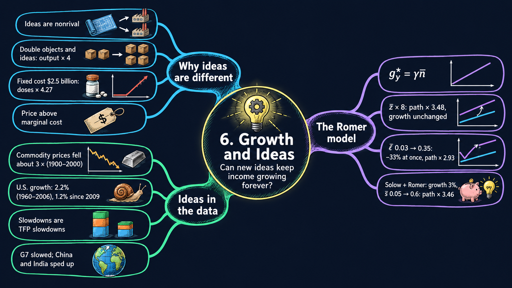
Learning goals

The Solow model of Chapter 5 could not explain sustained growth. This chapter adds the missing engine: new ideas. By the end of the chapter you will be able to:

explain why ideas are nonrival, show with exponents that nonrivalry means increasing returns, and show with a fixed cost why prices must lie above marginal cost if anyone is to pay for research;
derive the Romer model’s balanced growth path step by step: the stock of ideas, the level of income per person and the long-run growth rate $g_y^* = \gamma\bar{n}$, and the transition after a parameter change;
read the comparative statics as growth effects and level effects, including the hump-shaped effect of the research share, and run experiments with the Romer model and the combined Solow–Romer model;
derive the combined model’s growth rate $\tfrac{3}{2}\gamma\bar{n}$, its capital-output ratio and its level, and derive the growth-accounting decomposition;
read long-run data on commodity prices, U.S. growth and growth accounting;
simulate a model year by year with a for loop, draw ratio-scale charts in Plotly, and compute growth rates over periods with pandas;
go beyond the textbook’s data: compare 40 commodities and 185 countries with a picker of your own.

Model overview

In Chapter 5, Islandia got richer by building tools, but each extra boat added less than the one before, so tool building alone ran out of steam. Now an islander draws a better hull design. Harbor Boatworks can use that one drawing in every yard on the island at the same time, and the drawing never wears out. Can a steady stream of new ideas like this one keep Islandia getting richer year after year? This section answers with Paul Romer’s model of ideas, and we follow Islandia through every step.

The big idea

The question. Capital alone cannot sustain growth. What can keep income per person rising decade after decade?

The answer in one sentence. New ideas: because an idea is nonrival, it raises the output of every worker at once, so a research workforce that keeps growing keeps income per person growing.

What goes in and what comes out. We choose how productive research is, the share of people who do research, population growth, how much ideas matter in production and, once capital is back, the investment and depreciation rates. The model gives back the stock of ideas, the level of income per person on its balanced growth path, its long-run growth rate, and the path from any starting point.

Road map.

The economics of ideas: what makes ideas special, and why solving the model leads to increasing returns and prices above marginal cost.
The Romer model: the assumptions, the solution for the stock of ideas and long-run growth, and what the model predicts when research changes.
Combining Solow and Romer: capital comes back and amplifies the growth that ideas create.
Growth accounting: splitting measured growth into capital, labor composition and productivity.
Model in code: the key results as Python functions, checked with numbers.

Notation. A bar over a letter marks a parameter, a number we choose from outside the model; the exponent $\gamma$ (gamma) is a parameter too, written without a bar. Letters without a bar are endogenous variables, which the model determines. In the code we write z, l, n, gamma, s and d.

Symbol	Meaning	Type
$Y_t, A_t, N_t$	output, the stock of ideas and population in year $t$	endogenous
$L_{yt}, L_{at}$	workers who make goods and researchers who make ideas	endogenous
$K_t$	capital (combined model and growth accounting)	endogenous
$y_t, k_t$	output and capital per person, $Y_t/N_t$ and $K_t/N_t$	endogenous
$\gamma$	how much ideas matter: the degree of increasing returns	parameter
$\bar{z}$	research productivity: new ideas per researcher per year	parameter
$\bar{\ell}$	research share: the fraction of people who do research	parameter
$\bar{n}$	population growth rate	parameter
$\bar{s}, \bar{d}$	investment and depreciation rates (combined model)	parameters
$\bar{A}_0, \bar{N}_0, \bar{K}_0$	starting ideas, population and capital	parameters
$\bar{F}, c$	research (fixed) cost and the cost of each unit (first block)	parameters
$y_t^, A_t^$	a star marks the balanced growth path (BGP)	endogenous
$\Delta x_{t+1}$, $g_{xt}$	the change $x_{t+1}-x_t$, and the growth rate $\Delta x_{t+1}/x_t$	notation

The economics of ideas

Definitions

Objects and ideas. Romer splits all goods into two kinds. Objects are physical: land, oil, machines, buildings, workers. Ideas are instructions for arranging objects: a phone design, the formula of a medicine, a piece of software. On Islandia, the boats and nets are objects; the hull design is an idea.

Rival and nonrival. A good is rival when one person’s use leaves less of it for everyone else: a boat out at sea with one crew cannot carry a second crew at the same moment. Objects are rival, and that is why they are scarce. A good is nonrival when any number of people can use it at once without using it up. Ideas are nonrival: when a second yard builds from the hull design, the first yard has lost nothing. (Do not mix this up with excludability, the legal power to stop others from using a good. A patent can make an idea excludable, but it cannot make it rival.)

Production with ideas. Take the production function of Chapters 4 and 5 and put the stock of ideas $A_t$ where the productivity parameter $\bar{A}$ used to be:

\[Y_t = A_tK_t^{1/3}L_t^{2/3}.\]

Productivity now carries a time subscript, because new ideas keep adding to it.

Objects get used up when shared; ideas do not. Everything else in this chapter grows out of that difference.

Solving the model

Step 1: constant returns to objects. Scale both objects, capital and labor, by the same factor $\lambda > 0$, and hold the ideas fixed. The exponent rules (Appendix C.3) give $(\lambda K)^{1/3} = \lambda^{1/3}K^{1/3}$, so

\[A(\lambda K)^{1/3}(\lambda L)^{2/3} = \lambda^{1/3}\lambda^{2/3}\cdot AK^{1/3}L^{2/3} = \lambda^{1/3+2/3}\,Y = \lambda Y.\]

In words: the replication argument

To build twice as many boats, Harbor Boatworks can open a second yard that copies the first: new sheds, new tools, new workers. What it does not need is a second hull design. The one it already has is nonrival, so both yards work from the same drawing.

Step 2: increasing returns to objects and ideas together. Now scale the ideas too:

\[(\lambda A)(\lambda K)^{1/3}(\lambda L)^{2/3} = \lambda\cdot\lambda\cdot AK^{1/3}L^{2/3} = \lambda^2\,Y.\]

The logic needs nothing beyond nonrivalry. If copying the objects already doubles output, then also doubling the ideas must give more than double.

Key result: increasing returns

\[(\lambda A)(\lambda K)^{1/3}(\lambda L)^{2/3} = \lambda^2\,Y \tag{1}\]

Once ideas count as an input, scaling every input by $\lambda$ multiplies output by $\lambda^2$.

Islandia in numbers. If Islandia doubles its tools, its workers and its designs ($\lambda = 2$), it makes 4 times as much; if it triples all three, it makes 9 times as much.

Step 3: a fixed cost gives the same result. An idea is costly to discover and cheap to use afterwards. Let a firm pay a research cost $\bar{F}$ once, and then make each unit at a constant cost $c$. If it spends $X > \bar{F}$ in total, it makes $Y = (X-\bar{F})/c$ units. Dividing by $X$ gives the average product, output per dollar spent:

\[\frac{Y}{X} = \frac{X-\bar{F}}{cX} = \frac{1}{c}\left(1 - \frac{\bar{F}}{X}\right).\]

As spending grows, the fraction $\bar{F}/X$ shrinks, so output per dollar rises with scale. With no fixed cost, $Y/X = 1/c$ would never change. The antibiotic of Fig. 1 has $\bar{F}$ = 2.5 billion dollars and $c$ = 10 dollars a dose. Spending 3.6 billion buys 110 million doses, about 31 million per billion dollars. Spending twice that, 7.2 billion, buys 470 million doses, about 65 million per billion. Twice the input yields more than four times the output.

Step 4: pricing at marginal cost loses the fixed cost. The firm sells its $Y$ units at a price $p$. Its profit is revenue minus every cost:

\[\pi = pY - \bar{F} - cY = (p - c)\,Y - \bar{F}.\]

If competition drives the price down to marginal cost, $p = c$, profit is $-\bar{F}$: the research money is simply lost. Setting $\pi = 0$ and solving for $p$ gives the break-even price,

\[p = c + \frac{\bar{F}}{Y},\]

the marginal cost plus the research cost shared out over every unit sold. At the larger scale above, with $Y = 470$ million doses and $\bar{F} = 2{,}500$ million dollars, the firm needs at least $10 + 2{,}500/470 \approx 15.3$ dollars a dose.

Nonrival ideas mean increasing returns, and increasing returns mean that a price equal to marginal cost cannot pay for invention.

Check your understanding

1. Islandia scales its tools, its workers and its stock of designs all by $\lambda = 1.5$. By how much does output rise? And if only tools and workers grow by that factor?

Answer

By equation (1), output is multiplied by $1.5^2 = 2.25$ when all three grow. With the designs held fixed, step 1 gives constant returns to objects, so output is multiplied by just 1.5.

2. A rival copies the formula of the Fig. 1 antibiotic and sells it at 10 dollars, the marginal cost. Why can the inventor not match that price at 470 million doses?

Answer

At $p = c$ the inventor’s profit is $(p-c)Y - \bar{F} = -\bar{F}$, a loss of the whole 2.5 billion dollars spent on research. To break even it needs $p = c + \bar{F}/Y = 10 + 2{,}500/470 \approx 15.3$ dollars a dose. The copier never paid $\bar{F}$, which is why patents exist.

What the model predicts

Scale …	by	Output is multiplied by	Why
capital and labor only	2	2	constant returns to objects (step 1)
the stock of ideas only	2	2	output is proportional to $A$
objects and ideas	2	4	increasing returns, equation (1)
objects and ideas	3	9	increasing returns, equation (1)

Ideas, then nonrivalry, then increasing returns. Each link follows from the one before. Increasing returns are not assumed separately: they come out of nonrivalry as soon as ideas are counted as an input.
Average cost falls with scale. The cost of each unit is $X/Y = c + \bar{F}/Y$, so a bigger market spreads the research cost more thinly. The larger the market, the more ideas are worth inventing.
Perfect competition cannot pay for ideas. Research needs some wedge between price and marginal cost: patents and copyrights, trade secrets, or money from elsewhere, such as public research funding or prizes.
The wedge has a cost. A price above marginal cost turns away buyers who value the good at more than the cost of one more unit, but at less than the price. No single price can both reward the inventor and spread an existing idea as widely as possible.

Ideas need a reward above marginal cost, and that reward keeps some people from using them.

The Romer model

Assumptions

To see what ideas do on their own, the Romer model leaves capital out. Time runs in years, and Islandia has five endogenous variables: output $Y_t$, the stock of ideas $A_t$, workers who make goods $L_{yt}$, researchers $L_{at}$ and population $N_t$.

1. Making goods. Workers combine with the whole stock of ideas:

\[Y_t = A_t^{\gamma}L_{yt}.\]

With ideas held fixed, returns to the one object, workers, are constant: twice the workers make twice the goods. Scaling ideas and workers together by $\lambda$ multiplies output by $\lambda^{\gamma}\cdot\lambda = \lambda^{1+\gamma}$. The extra $\gamma$ is the degree of increasing returns, and it also tells us how much ideas matter in production.

2. Making ideas. Each researcher adds $\bar{z}$ new ideas a year to a stock that starts at $\bar{A}_0$:

\[\Delta A_{t+1} \equiv A_{t+1} - A_t = \bar{z}L_{at}.\]

Picture $A_t$ as Islandia’s library of blueprints. Researchers add new drawings every year, and since ideas do not wear out, no drawing is ever thrown away.

3. Using people. Every islander either makes goods or does research:

\[L_{yt} + L_{at} = N_t.\]

4. Population. The population grows at a constant rate $\bar{n}$ from its starting level $\bar{N}_0$, so $N_t = \bar{N}_0(1+\bar{n})^t$:

\[\frac{\Delta N_{t+1}}{N_t} = \bar{n}.\]

5. Allocation. A fixed share $\bar{\ell}$ of the population works in research:

\[L_{at} = \bar{\ell}N_t.\]

This rule of thumb plays the part of the constant investment rate $\bar{s}$ in the Solow model. In Romer’s original work, markets with patents and monopoly profits decide how many people do research, and they tend to pick too few.

Equation	Name	Parameters it uses
$Y_t = A_t^{\gamma}L_{yt}$	production of goods	$\gamma$
$\Delta A_{t+1} = \bar{z}L_{at}$	production of ideas	$\bar{z}$, and $\bar{A}_0$ to start
$L_{yt} + L_{at} = N_t$	resource constraint for people	none
$\Delta N_{t+1}/N_t = \bar{n}$	population growth	$\bar{n}$, and $\bar{N}_0$ to start
$L_{at} = \bar{\ell}N_t$	allocation of people	$\bar{\ell}$

Islanders either make goods or make ideas, and the library of ideas only ever grows.

Solving the model

Step 1: the two kinds of workers. The allocation rule gives $L_{at} = \bar{\ell}N_t$ directly. Substituting it into the resource constraint gives $L_{yt} = N_t - \bar{\ell}N_t = (1-\bar{\ell})N_t$. Both groups depend only on population, which grows at $\bar{n}$.

Step 2: output per person. Divide the production of goods by $N_t$ and use step 1:

\[y_t \equiv \frac{Y_t}{N_t} = \frac{A_t^{\gamma}(1-\bar{\ell})N_t}{N_t} = A_t^{\gamma}(1-\bar{\ell}).\]

In words: the whole library counts

An islander’s income depends on the whole stock of ideas, not on ideas per person. One new hull design helps every yard on the island, however many islanders there are. In the Solow model it was the other way round: $y = \bar{A}k^{1/3}$ depends on capital per person, because a boat helps only the crew that sails it.

Step 3: the growth rate of ideas. Divide the production of ideas by $A_t$ and use $L_{at} = \bar{\ell}N_t$:

\[g_{At} \equiv \frac{\Delta A_{t+1}}{A_t} = \frac{\bar{z}L_{at}}{A_t} = \frac{\bar{z}\bar{\ell}N_t}{A_t}.\]

Multiplying both sides by $A_t$ and dividing by $g_{At}$ writes the stock of ideas as $A_t = \bar{z}\bar{\ell}N_t/g_{At}$: the yearly flow of new ideas divided by their growth rate.

Step 4: the balanced growth path. On a balanced growth path (BGP), every growth rate stays constant. With a constant $g_A^*$, the expression above makes $A_t$ a fixed number, $\bar{z}\bar{\ell}/g_A^*$, times $N_t$. A constant times $N_t$ grows exactly as fast as $N_t$, so $g_A^* = \bar{n}$: ideas grow as fast as the number of researchers, and the number of researchers grows as fast as the population. Putting $g_A^* = \bar{n}$ back in gives $A_t^* = \bar{z}\bar{\ell}N_t/\bar{n}$.

The result also holds exactly in yearly steps: $A_{t+1}^* - A_t^* = \bar{z}\bar{\ell}(N_{t+1}-N_t)/\bar{n} = \bar{z}\bar{\ell}\,\bar{n}N_t/\bar{n} = \bar{z}\bar{\ell}N_t$, which is precisely the number of new ideas that researchers produce.

Key result: income per person and the stock of ideas

\[y_t = A_t^{\gamma}(1-\bar{\ell}) \tag{2}\]

\[A_t^* = \frac{\bar{z}\bar{\ell}N_t}{\bar{n}} \tag{3}\]

Equation (2) holds in every year. Equation (3) says that on the BGP the stock of ideas is proportional to the number of researchers, $\bar{\ell}N_t$: more people at work on ideas means more ideas.

Step 5: the level of income per person. Substitute equation (3) into equation (2):

\[y_t^* = (1-\bar{\ell})\left(\frac{\bar{z}\bar{\ell}N_t}{\bar{n}}\right)^{\gamma}.\]

Because $(ab)^{\gamma} = a^{\gamma}b^{\gamma}$, this is also $y_t^* = (1-\bar{\ell})\,\bar{\ell}^{\gamma}\left(\bar{z}N_t/\bar{n}\right)^{\gamma}$, where $\bar{\ell}$ shows up twice. Income per person rises with the number of researchers to the power $\gamma$. And since researchers are a fixed share of the population, it also rises with the size of the population itself.

Step 6: the long-run growth rate. Apply the growth rule for powers, $g_{x^a} = a\,g_x$ (Appendix C.5), to equation (2). The factor $1-\bar{\ell}$ is constant and adds nothing, so $g_{yt} = \gamma\,g_{At}$. On the BGP $g_A^* = \bar{n}$, so $g_y^* = \gamma\bar{n}$. Equation (4) agrees: its only part that changes over time is $N_t^{\gamma}$, which grows at $\gamma\bar{n}$.

Key result: the balanced growth path

\[y_t^* = (1-\bar{\ell})\left(\frac{\bar{z}\bar{\ell}N_t}{\bar{n}}\right)^{\gamma} \tag{4}\]

\[g_y^* = \gamma\bar{n} \tag{5}\]

Long-run growth is the degree of increasing returns times the growth rate of the research workforce.

Islandia in numbers. With $\gamma = 0.6$ and $\bar{n} = 0.05$ (Figs. 3 and 4), output per person grows by $0.6\times0.05 = 3$ percent a year; with $\gamma = 0.7$ (Fig. 2) it grows by 3.5 percent. In yearly steps the exact factor is $(1+\bar{n})^{\gamma}$, for example $1.05^{0.6} \approx 1.0297$.

In words: the engine the Solow model lacked

Each year Islandia has more people, so it has more researchers, so it adds more blueprints to the library. Every blueprint helps every islander at once. Growth never runs out, because the library has no diminishing returns of its own: it keeps pace with a research workforce that keeps growing.

Step 7: off the balanced growth path. Step 3 holds every year, on the BGP or off it. Multiply and divide its right side by $\bar{n}$, and use equation (3):

\[g_{At} = \frac{\bar{z}\bar{\ell}N_t}{A_t} = \bar{n}\cdot\frac{\bar{z}\bar{\ell}N_t/\bar{n}}{A_t} = \bar{n}\,\frac{A_t^*}{A_t}. \tag{6}\]

When the stock of ideas is below its BGP value ($A_t < A_t^*$), ideas grow faster than $\bar{n}$; when it is above, they grow more slowly. Either way the gap closes, because the fast growth pushes $A_t$ toward $A_t^*$. This is the Romer model’s form of the principle of transition dynamics: the further an economy falls short of its BGP, the faster it grows, and above the BGP it grows more slowly. Output per person then grows at $g_{yt} = \gamma\,g_{At}$ (exactly, in yearly steps, by the factor $(1+g_{At})^{\gamma}$).

Ideas grow as fast as the research workforce, so income per person grows at gamma times population growth, for ever.

Check your understanding

1. With $\gamma = 0.6$, Islandia’s population growth slows from 5 percent to 2 percent a year. What happens to long-run growth of output per person?

Answer

By equation (5), $g_y^* = \gamma\bar{n}$ falls from $0.6\times0.05 = 3$ percent to $0.6\times0.02 = 1.2$ percent a year. Fewer new islanders each year means fewer new researchers, so fewer new ideas.

2. Islandia’s starting population $\bar{N}_0$ were twice as large, with every parameter unchanged. Would it grow faster in the long run? Would it be richer?

Answer

It would not grow faster: $\bar{N}_0$ does not appear in equation (5). It would be richer: $N_t$ doubles in every year, so by equation (4) the BGP is higher by the factor $2^{\gamma} = 2^{0.6} \approx 1.52$. Twice the people means twice the researchers, and their ideas serve everyone.

What the model predicts

Growth effects and level effects. A growth effect changes the long-run growth rate of equation (5). A level effect moves the BGP of equation (4) up or down without changing its slope on a ratio scale. Taking logs of equation (4) (Appendix C.4),

\[\ln y_t^* = \ln(1-\bar{\ell}) + \gamma\ln\bar{\ell} + \gamma\ln\bar{z} + \gamma\ln N_t - \gamma\ln\bar{n}.\]

Each coefficient is an elasticity: the percentage change in $y_t^*$ when that parameter rises by 1 percent. For $\bar{\ell}$, use $\frac{d\ln(1-\bar{\ell})}{d\ln\bar{\ell}} = -\frac{\bar{\ell}}{1-\bar{\ell}}$ (Appendix C.7).

A permanent rise in …	Long-run growth $g_y^*$	Elasticity of the BGP level $y_t^*$	Output per person on impact
research productivity $\bar{z}$	unchanged	$+\gamma$	unchanged
research share $\bar{\ell}$	unchanged	$\gamma - \dfrac{\bar{\ell}}{1-\bar{\ell}}$ (positive for small $\bar{\ell}$)	falls by the factor $\dfrac{1-\bar{\ell}'}{1-\bar{\ell}}$
population growth $\bar{n}$	rises by $\gamma\,\Delta\bar{n}$	$-\gamma$, at a given $N_t$	unchanged
initial population $\bar{N}_0$	unchanged	$+\gamma$	unchanged

Experiment 1: Islandia’s researchers become more productive (Fig. 3). Long-run growth stays at $\gamma\bar{n}$, because $\bar{z}$ does not enter equation (5). By equation (4), the BGP rises by the factor $(\bar{z}'/\bar{z})^{\gamma}$: with $\gamma = 0.6$, an eightfold rise in $\bar{z}$ lifts it by $8^{0.6} \approx 3.48$. At the moment of the change, the library holds only what past research put there, so output per person does not jump. But $A_t^*$ is now eight times $A_t$, and by equation (6) ideas grow by $0.05\times8 = 40$ percent in the first year. Output per person grows by $1.40^{0.6} - 1 \approx 22$ percent, then more and more slowly as $A_t$ catches up with $A_t^*$.

Experiment 2: more islanders go into research (Fig. 4). Long-run growth is again unchanged. The BGP level contains $\bar{\ell}$ twice: more researchers make more ideas ($\bar{\ell}^{\gamma}$), but fewer islanders are left to make goods ($1-\bar{\ell}$). The elasticity $\gamma - \bar{\ell}/(1-\bar{\ell})$ equals zero where $\bar{\ell}/(1-\bar{\ell}) = \gamma$, that is, at

\[\bar{\ell} = \frac{\gamma}{1+\gamma},\]

which is $0.6/1.6 = 0.375$ for $\gamma = 0.6$ (Appendix C.8). Below that share, a larger $\bar{\ell}$ lifts the BGP; above it, the BGP falls. The relationship is hump shaped. On impact the stock of ideas is given, so by equation (2) output per person falls with $1-\bar{\ell}$. Raising $\bar{\ell}$ from 0.03 to 0.35 cuts output per person at once by the factor $0.65/0.97 \approx 0.67$, about 33 percent. In the long run the BGP is higher by $\dfrac{0.65\times0.35^{0.6}}{0.97\times0.03^{0.6}} \approx 2.93$. In between, Islandia sits far below its new BGP and grows fast.

A model of the world’s ideas. Equation (4) seems to say that a populous country should be far richer than a small one. That reading is wrong, because ideas travel through trade, multinational firms, licenses and migration. Islandia builds from designs drawn on Mainland as well as its own. So the Romer model describes the ideas of the whole world, and $N_t$ counts everyone, anywhere, who can create them. Why countries grow at different rates is a question for the combined model below.

Why ideas grow with the number of researchers, not faster. Romer’s original version let research raise the growth rate of ideas instead of their number: $\Delta A_{t+1}/A_t = \bar{z}L_{at}$. Then $g_{At} = \bar{z}\bar{\ell}N_t$ would itself grow at the rate $\bar{n}$, and growth of income per person would keep speeding up without limit. U.S. growth has stayed close to 2 percent a year for more than a century, with no such acceleration. The version used here keeps the insights and removes this problem.

Better or more research raises the level of Islandia’s path; only faster population growth changes its slope.

Check your understanding

1. Islandia’s research productivity doubles, with $\gamma = 0.6$ and $\bar{n} = 0.05$. How much higher is the new BGP? How fast do ideas and output per person grow in the first year?

Answer

By equation (4), the BGP rises by $2^{0.6} \approx 1.52$. Right after the change, $A_t^* = 2A_t$, so by equation (6) ideas grow by $0.05\times2 = 10$ percent, and output per person by $1.10^{0.6} - 1 \approx 5.9$ percent. Long-run growth stays at 3 percent.

2. With $\gamma = 0.6$, Islandia already has 40 percent of its people in research. Would moving more islanders into research raise its BGP?

Answer

No. The level effect peaks at $\bar{\ell} = \gamma/(1+\gamma) = 0.375$. At 40 percent Islandia is already past the top of the hump, so the goods lost from fewer workers outweigh the extra ideas.

Combining Solow and Romer

Assumptions

Now Islandia’s tools come back. The combined model has six endogenous variables, $Y_t$, $K_t$, $A_t$, $L_{yt}$, $L_{at}$ and $N_t$, and six equations:

Equation	Name	Comes from
$Y_t = A_t^{\gamma}K_t^{1/3}L_{yt}^{2/3}$	production of goods	both models
$\Delta K_{t+1} = \bar{s}Y_t - \bar{d}K_t$	capital accumulation, from $\bar{K}_0$	Solow
$\Delta A_{t+1} = \bar{z}L_{at}$	production of ideas, from $\bar{A}_0$	Romer
$L_{yt} + L_{at} = N_t$	resource constraint for people	Romer
$L_{at} = \bar{\ell}N_t$	allocation of people	Romer
$\Delta N_{t+1}/N_t = \bar{n}$	population growth, from $\bar{N}_0$	Romer

Returns to the two objects, capital and workers, are constant (the exponents $1/3$ and $2/3$ sum to one), and they become increasing once ideas are counted. Research uses only people. Letting it use tools too would lengthen the algebra without changing any result.

Solving the model

Step 1: output per person. Divide the production function by $N_t$, written as $N_t = N_t^{1/3}N_t^{2/3}$, and use $L_{yt} = (1-\bar{\ell})N_t$:

\[y_t = \frac{A_t^{\gamma}K_t^{1/3}L_{yt}^{2/3}}{N_t^{1/3}N_t^{2/3}} = A_t^{\gamma}\left(\frac{K_t}{N_t}\right)^{1/3}\left(\frac{L_{yt}}{N_t}\right)^{2/3} = A_t^{\gamma}k_t^{1/3}(1-\bar{\ell})^{2/3},\]

where $k_t \equiv K_t/N_t$ is capital per person.

Step 2: growth rates. By the growth rules for a product and for a power (Appendix C.5), the growth rate of $y_t$ adds up the growth rates of its factors, each multiplied by its exponent. The constant $(1-\bar{\ell})^{2/3}$ contributes nothing:

\[g_{yt} = \gamma\,g_{At} + \tfrac{1}{3}\,g_{kt}.\]

Step 3: ideas. Producing ideas and allocating people work exactly as in the Romer model, so the same steps give $g_A^* = \bar{n}$ and the BGP stock of ideas in equation (3).

Step 4: capital. Divide capital accumulation by $K_t$:

\[g_{Kt} = \frac{\Delta K_{t+1}}{K_t} = \bar{s}\,\frac{Y_t}{K_t} - \bar{d}.\]

On a BGP $g_{Kt}$ is constant, and so are $\bar{s}$ and $\bar{d}$, so $Y_t/K_t$ must be constant as well. A ratio stays put only when its top and bottom grow at the same rate, so $g_K^* = g_Y^*$. Subtracting $\bar{n}$ from both sides (the growth rule for a ratio) gives $g_k^* = g_y^*$: capital per person grows as fast as output per person.

Step 5: the long-run growth rate. Put $g_A^* = \bar{n}$ and $g_k^* = g_y^*$ into step 2, and solve for $g_y^*$:

\[g_y^* = \gamma\bar{n} + \tfrac{1}{3}g_y^* \quad\Longrightarrow\quad \tfrac{2}{3}\,g_y^* = \gamma\bar{n} \quad\Longrightarrow\quad g_y^* = \tfrac{3}{2}\gamma\bar{n}.\]

Key result: growth in the combined model

\[g_y^* = \tfrac{3}{2}\gamma\bar{n} \tag{7}\]

Ideas still set long-run growth, but capital multiplies it by $3/2$.

Islandia in numbers. With the values of Fig. 8, $\gamma = 2/3$ and $\bar{n} = 0.03$, output per person grows by $\tfrac{3}{2}\times\tfrac{2}{3}\times0.03 = 3$ percent a year, against $\gamma\bar{n} = 2$ percent in the Romer model. Total output grows at $g_Y^* = g_y^* + \bar{n}$, about 6 percent (exactly $1.03\times1.03 - 1 = 6.09$ percent in yearly steps).

In words: capital as an amplifier

A new design lets Islandia make more. Part of the extra output becomes new tools, and the new tools raise output again, by a third as much. Part of that is turned into tools in turn, and so on. The rounds add up to $1 + \tfrac{1}{3} + \tfrac{1}{9} + \dots = \tfrac{3}{2}$. Tools cannot drive growth on their own, but they magnify whatever ideas do.

Step 6: the capital-output ratio. On the BGP $g_K^* = g_Y^*$. Put this into step 4, $g_Y^* = \bar{s}\,Y_t^*/K_t^* - \bar{d}$, add $\bar{d}$ to both sides and solve for $K_t^*/Y_t^*$:

\[\frac{K_t^*}{Y_t^*} = \frac{\bar{s}}{g_Y^* + \bar{d}}. \tag{8}\]

This is the Solow capital-output ratio $\bar{s}/\bar{d}$ of Chapter 5, with $g_Y^* + \bar{d}$ in place of $\bar{d}$. Investment now has to replace the tools that wear out and keep the stock of tools growing as fast as output. With $\bar{s} = 0.05$, $\bar{d} = 0.02$ and $g_Y^* = 0.0609$, the ratio is $0.05/0.0809 \approx 0.62$.

Step 7: the level of income per person. Equation (8) says $K_t^* = \frac{\bar{s}}{g_Y^*+\bar{d}}\,Y_t^*$. Substitute it into the production function:

\[Y_t^* = (A_t^*)^{\gamma}\left(\frac{\bar{s}}{g_Y^*+\bar{d}}\right)^{1/3}(Y_t^*)^{1/3}L_{yt}^{2/3}.\]

Divide both sides by $(Y_t^*)^{1/3}$, leaving $(Y_t^*)^{2/3}$ on the left, and raise both sides to the power $3/2$. The exponents multiply: $\gamma\times\tfrac{3}{2}$, $\tfrac{1}{3}\times\tfrac{3}{2} = \tfrac{1}{2}$ and $\tfrac{2}{3}\times\tfrac{3}{2} = 1$:

\[Y_t^* = (A_t^*)^{3\gamma/2}\left(\frac{\bar{s}}{g_Y^*+\bar{d}}\right)^{1/2}L_{yt}.\]

Finally, divide by $N_t$ with $L_{yt}/N_t = 1-\bar{\ell}$:

\[y_t^* = \left(\frac{\bar{s}}{g_Y^*+\bar{d}}\right)^{1/2}(A_t^*)^{3\gamma/2}\,(1-\bar{\ell}).\]

The textbook prints this result with the exponent $3/2$ on $A_t^*$ (and with a constant labor force in the denominator), which holds only in the special case $\gamma = 1$. For any $\gamma$, the derivation above gives $3\gamma/2$.

Key result: the level of the balanced growth path

\[y_t^* = \left(\frac{\bar{s}}{g_Y^*+\bar{d}}\right)^{1/2}(A_t^*)^{3\gamma/2}\,(1-\bar{\ell}) \tag{9}\]

With $A_t^*$ from equation (3), the full solution in parameters and population is

\[y_t^* = \left(\frac{\bar{s}}{g_Y^*+\bar{d}}\right)^{1/2}(1-\bar{\ell})\left(\frac{\bar{z}\bar{\ell}N_t}{\bar{n}}\right)^{3\gamma/2}.\]

Its only part that changes over time, $N_t^{3\gamma/2}$, grows at $\tfrac{3}{2}\gamma\bar{n}$, which confirms equation (7). As in the Romer model, income rises with the whole stock of ideas; as in the Solow model, it rises with $\bar{s}^{1/2}$.

Islandia in numbers. If Islandia invested twice as much, its income per person would rise only by the factor $2^{1/2} \approx 1.41$.

Ideas set the long-run growth rate; saving and depreciation, as in Solow, only set how high the path lies.

Check your understanding

1. Suppose ideas mattered less in Islandia, with $\gamma = 1/3$ instead of $2/3$, and $\bar{n} = 0.03$. What is long-run growth in the combined model, and in the Romer model without capital?

Answer

By equation (7), $g_y^* = \tfrac{3}{2}\times\tfrac{1}{3}\times0.03 = 1.5$ percent a year. Without capital, equation (5) gives $\gamma\bar{n} = 1$ percent. Capital multiplies the growth from ideas by $3/2$ in both cases.

2. Islandia starts saving a larger share of its output. Why does that not change its long-run growth rate?

Answer

The investment rate $\bar{s}$ does not appear in equation (7). A higher $\bar{s}$ raises the capital-output ratio of equation (8), and so the level of the path in equation (9), but tools still face diminishing returns. Only new ideas keep growth going.

What the model predicts

Comparative statics. Take logs of the full solution: $\ln y_t^* = \tfrac{1}{2}\ln\bar{s} - \tfrac{1}{2}\ln(g_Y^*+\bar{d}) + \ln(1-\bar{\ell}) + \tfrac{3\gamma}{2}\left(\ln\bar{z} + \ln\bar{\ell} + \ln N_t - \ln\bar{n}\right)$.

A permanent rise in …	Long-run growth $g_y^*$	Elasticity of the BGP level $y_t^*$	With the Fig. 8 values
investment rate $\bar{s}$	unchanged	$+\tfrac{1}{2}$	$+0.5$
depreciation rate $\bar{d}$	unchanged	$-\tfrac{1}{2}\cdot\dfrac{\bar{d}}{g_Y^*+\bar{d}}$	$-0.12$
research productivity $\bar{z}$	unchanged	$+\tfrac{3\gamma}{2}$	$+1$
research share $\bar{\ell}$	unchanged	$\tfrac{3\gamma}{2} - \dfrac{\bar{\ell}}{1-\bar{\ell}}$	$+0.89$
population growth $\bar{n}$	rises by $\tfrac{3}{2}\gamma\,\Delta\bar{n}$	changes the path’s slope	—
starting capital $\bar{K}_0$ or ideas $\bar{A}_0$	unchanged	none: only the transition	—

Every parameter other than $\gamma$ and $\bar{n}$ has only a level effect. Each level elasticity tied to ideas is $3/2$ times its Romer value, for the same reason as in equation (7): capital amplifies whatever ideas do.

Transition dynamics. Step 4 holds in every year, and on the BGP $\bar{s} = (g_Y^*+\bar{d})\,K_t^*/Y_t^*$ by equation (8). Substituting,

\[g_{Kt} = \bar{s}\,\frac{Y_t}{K_t} - \bar{d} = (g_Y^*+\bar{d})\,\frac{K_t^*/Y_t^*}{K_t/Y_t} - \bar{d}.\]

When capital is low relative to output ($K_t/Y_t$ below its BGP value), capital grows faster than $g_Y^*$, and output with it; when it is high, both grow more slowly. That is the combined model’s principle of transition dynamics: the larger the percentage gap below the BGP, the faster the growth, and above the BGP growth is slower. Suppose Islandia raises $\bar{s}$ from 0.05 to 0.6 (Fig. 8). The BGP capital-output ratio becomes 12 times larger overnight, while the actual ratio has not moved. In the first year capital grows by $0.0809\times12 - 0.02 \approx 95$ percent, and output per person by about 26 percent (the code below confirms both). Growth then slows back toward 3 percent, and in the long run output per person is $(0.6/0.05)^{1/2} = \sqrt{12} \approx 3.46$ times its old path.

Why growth rates differ across countries. In the long run every country shares the growth rate of world ideas, equation (7). Over any decade, though, countries differ in how far they are from their BGPs, and policies that change $\bar{s}$, $\bar{\ell}$ or other parameters open new gaps. So the model accounts both for the steady growth of the richest countries and for decades of fast catch-up growth in countries such as Japan or South Korea.

A country far below its balanced growth path grows fast for a while, then settles back to the world’s pace.

Check your understanding

1. Instead of 0.6, Islandia raises its investment rate from 0.05 to 0.2, with the Fig. 8 values otherwise. How much higher is its new path in the long run, and what is long-run growth of output per person?

Answer

By equation (9), the path rises by $(0.2/0.05)^{1/2} = 2$: Islandia ends up twice as rich. Long-run growth does not change: by equation (7) it stays at $\tfrac{3}{2}\times\tfrac{2}{3}\times0.03 = 3$ percent a year. In between, growth is faster than 3 percent while capital catches up.

Growth accounting

Definitions

Growth accounting uses the combined production function with $\gamma = 1$, so that $A_t$ is plain total factor productivity (TFP):

\[Y_t = A_tK_t^{1/3}L_{yt}^{2/3}.\]

Here $L_t$ is the total number of hours worked, and $L_{yt}$ is the effective labor input, which also changes when Islandia’s workforce becomes more educated or more experienced. As before, $g_{Xt} \equiv \Delta X_{t+1}/X_t$ for each variable $X$.

Solving the model

Step 1: the growth rate of output. Take logs of the production function (Appendix C.4): $\ln Y_t = \ln A_t + \tfrac{1}{3}\ln K_t + \tfrac{2}{3}\ln L_{yt}$. A change in a log is approximately a growth rate (Appendix C.5), so the change of both sides from one year to the next is

\[g_{Yt} = g_{At} + \tfrac{1}{3}g_{Kt} + \tfrac{2}{3}g_{L_yt}.\]

Each input contributes its growth rate times its exponent; exponents below one reflect diminishing returns to each input.

Step 2: per hour worked. Subtract $g_{Lt}$ from both sides. On the right, write it as $g_{Lt} = \tfrac{1}{3}g_{Lt} + \tfrac{2}{3}g_{Lt}$, so that each input gives up its share:

\[\underbrace{g_{Yt}-g_{Lt}}_{\text{output per hour}} = \underbrace{\tfrac{1}{3}(g_{Kt}-g_{Lt})}_{\text{capital per hour}} + \underbrace{\tfrac{2}{3}(g_{L_yt}-g_{Lt})}_{\text{labor composition}} + \underbrace{g_{At}}_{\text{TFP growth}}.\]

Key result: growth accounting

\[g_{Yt}-g_{Lt} = \tfrac{1}{3}(g_{Kt}-g_{Lt}) + \tfrac{2}{3}(g_{L_yt}-g_{Lt}) + g_{At} \tag{10}\]

Growth of output per hour splits into three parts: more capital per hour, a better-skilled workforce, and TFP growth.

Islandia in numbers. If output per hour grows by 2.0 percent a year, capital per hour by 2.4 percent, and labor composition adds 0.2 points, capital per hour contributes $\tfrac{1}{3}\times2.4 = 0.8$ points, and TFP growth is $2.0 - 0.8 - 0.2 = 1.0$ point: half of all growth.

Step 3: TFP as the residual. Output, capital, hours and labor composition can all be measured; TFP cannot. So equation (10) is read the other way round: TFP growth is what remains of output-per-hour growth once the two measured contributions are taken out,

\[g_{At} = (g_{Yt}-g_{Lt}) - \tfrac{1}{3}(g_{Kt}-g_{Lt}) - \tfrac{2}{3}(g_{L_yt}-g_{Lt}).\]

That is why TFP growth is also called the Solow residual.

In words: what is left over

Islandia’s statisticians can count hours, tools and schooling, but nobody can count blueprints. So they measure everything they can, credit each piece its share of growth, and call whatever is left over TFP growth. The residual is our best gauge of new ideas, and also of everything else we failed to measure.

Check your understanding

1. Islandia’s output per hour grows by 1.5 percent a year, capital per hour by 1.8 percent, and labor composition adds 0.3 points. How much is TFP growth, and what share of growth is it?

Answer

By equation (10), capital per hour contributes $\tfrac{1}{3}\times1.8 = 0.6$ points, so TFP growth is $1.5 - 0.6 - 0.3 = 0.6$ points, or 40 percent of the growth in output per hour.

What the model predicts

A worked example. The numbers in the box above: with output per hour up 2.0 percent and TFP growth of 1.0 point, ideas and other unmeasured gains account for half of all growth.
Slowdowns are TFP slowdowns. In the U.S. data of Fig. 6, periods of slow productivity growth are mostly periods of slow TFP growth: the part that the Romer model ties to new ideas.
Accounting is not causation. On the BGP of the combined model with $\gamma = 1$, step 5 above gives $g_y^* = \tfrac{3}{2}g_A^*$, and capital per hour grows as fast as output per hour. Equation (10) would then credit one third of growth to capital, $\tfrac{1}{3}\times\tfrac{3}{2}g_A^* = \tfrac{1}{2}g_A^*$, although ideas cause all of it: the tools exist only because TFP growth made them worth building.
A test for balanced growth. On a BGP, output per hour and capital per hour grow at the same rate. An economy whose capital per hour grows much faster than its output per hour is still in transition, below its BGP.

TFP is the growth left unexplained by measured inputs, and much of what capital seems to explain is really caused by ideas.

Recap

Ideas are nonrival: sharing them costs nothing, so objects and ideas together have increasing returns (Fig. 1), and a price equal to marginal cost cannot cover a fixed research cost.
The Romer model: ideas grow as fast as the research workforce, so output per person grows at $g_y^* = \gamma\bar{n}$ for ever (the straight line on a ratio scale in Figs. 2–4).
Growth effects and level effects: better research or a different research share moves the level of the path, not its slope, and the research share has a hump-shaped effect (Fig. 3, Fig. 4).
Capital amplifies ideas: in the combined model $g_y^* = \tfrac{3}{2}\gamma\bar{n}$, and saving more lifts only the level (Fig. 8).
Growth accounting splits growth into capital, labor composition and the TFP residual; slowdowns are mostly TFP slowdowns (Fig. 6).

Model in code

Now we turn the Key results into Python. The section has four parts: the setup (folded, because it is the same in every chapter), the model as functions, numerical checks of the Key results, and the drawing and data tools that the figures use (folded too). Run its cells once, in order. Every later section of the notebook reuses them.

Setup

Run the setup cells once, before anything else. They load the Python libraries, give every chart the same look, store the address of the chapter’s data and define four helpers that only the book website needs. You can use the notebook without reading them; open the box if you are curious.

Show the setup code

The first cell loads the libraries and sets the look of the charts. Its comments explain each step.

# @title Setup: libraries, chart colors and the data location
# Text after a "#" is a comment: Python ignores it, it is there for human readers.

# Step 1: load the libraries. `import` loads a library, a toolbox written by
# other people, and `as np` gives it a short nickname, so the code stays short.
import numpy as np                              # numbers and arrays
import pandas as pd                             # data tables
import plotly.express as px                     # quick charts from data tables
import plotly.graph_objects as go               # charts built piece by piece
import plotly.io as pio                         # settings shared by every chart
from plotly.subplots import make_subplots       # several panels in one figure
# sliders, buttons and menus for the interactive figures
from ipywidgets import interact, fixed, FloatSlider, ToggleButtons, Dropdown, SelectMultiple

# Step 2: one light blue/green look for every chart
BLUE, TEAL, GREEN, GRAY = "#16528c", "#008070", "#7fb23a", "#8a96a3"
pio.templates.default = "plotly_white"
# the same chart size in Colab and on the website
pio.templates["plotly_white"].layout.update(width=860, height=480)
px.defaults.color_discrete_sequence = [BLUE, TEAL, GREEN, "#5aa0d8", "#0b4f47"]
WIDE = {"description_width": "initial"}         # show the full slider labels

# Step 3, Colab only: let Plotly charts appear inside the interactive widgets.
# `try` runs the indented lines; if the import fails (we are not in Colab),
# `except` skips them.
try:
    import google.colab
    google.colab.output.enable_custom_widget_manager()
except ImportError:
    pass                                        # not running in Colab: nothing to do

# Step 4: the data files of this chapter live in the book's GitHub repository
DATA_URL = "https://raw.githubusercontent.com/quarcs-lab/macro102-site/main/data/ch06/"

The website cannot run Python, so each interactive figure also gets a version with a precomputed slider. The next helper builds those versions. Run it and move on.

# @title Helper for the website versions (run this cell; you do not need to read it)
def slider_figure(make_figure, name, values, start, label=None):
    """Join precomputed versions of a figure with one slider (the website cannot run Python).

    Arguments
        make_figure : the function that draws the figure, e.g. romer_bgp
        name        : the argument the slider moves, e.g. "gamma"
        values      : the values of that argument to precompute
        start       : the value shown first
        label       : the slider's label (the argument name if None)
    Returns
        one Plotly figure with all versions and a slider that shows one at a time
    """
    # Step 1: draw the figure once for every value
    figures = [make_figure(**{name: v}) for v in values]
    first = values.index(start)
    # Step 2: copy every curve into one figure; only the start value's are visible
    fig = go.Figure(layout=figures[first].layout)
    owner = []                                  # which figure each trace comes from
    for i, f in enumerate(figures):
        for trace in f.data:
            trace.visible = (i == first)
            fig.add_trace(trace)
            owner.append(i)
    # Step 3: one slider step per value: its curves, title, labels and shapes
    steps = []
    for i, f in enumerate(figures):
        layout = {"title": f.layout.title.to_plotly_json(),
                  "annotations": [a.to_plotly_json() for a in f.layout.annotations],
                  "shapes": [s.to_plotly_json() for s in f.layout.shapes]}
        visible = [o == i for o in owner]
        steps.append(dict(method="update", label=str(values[i]), args=[{"visible": visible}, layout]))
    fig.update_layout(sliders=[dict(active=first, steps=steps, pad=dict(t=60),
                                    currentvalue=dict(prefix=(label or name) + " = "))])
    return fig

The multi-country charts have three more website helpers. region_menu adds a menu of world regions to a chart that holds many countries, because a legend with 180 names would be unreadable. region_groups lists the countries that each view of that menu shows together, so that we can give them different colors. legend_menu keeps the textbook’s lines on, puts the others in the legend, and adds two reset buttons.

# @title Helpers for the website versions with many countries (run this cell; you do not need to read it)
def region_menu(fig, regions, shown, label=None):
    """Add a region menu: the countries in `shown` stay on, the chosen region's go into the legend.

    The website cannot run Python, so this menu replaces the Colab country picker: pick a region,
    then click a country in the legend to add it.

    Arguments
        fig     : a Plotly figure with one trace per country
        regions : maps each country (trace name) to its region
        shown   : the countries that stay drawn in every view
        label   : the name of the first menu entry (the textbook countries if None)
    Returns
        the same figure, with only `shown` drawn and the region menu above the plot
    """
    # Step 1: the trace names, and each region once, A to Z
    names = [trace.name for trace in fig.data]
    groups = sorted(set(regions[n] for n in names if n in regions))
    # Step 2: for each menu entry, which traces are drawn, in the legend only, or hidden
    buttons = []
    for group in [label or "Textbook: " + ", ".join(shown)] + groups:
        visible = []
        for n in names:
            if n in shown:
                visible.append(True)                    # a textbook country: drawn
            elif regions.get(n) == group:
                visible.append("legendonly")            # in this region: a click away
            else:
                visible.append(False)                   # another region: hidden
        buttons.append(dict(label=group, method="restyle", args=[{"visible": visible}]))
    # Step 3: start with the textbook countries only, and add the menu
    for trace in fig.data:
        trace.visible = True if trace.name in shown else False
    fig.update_layout(updatemenus=[dict(buttons=buttons, active=0, direction="down", showactive=True,
                                        x=0, xanchor="left", y=1.02, yanchor="bottom")],
                      margin=dict(t=120), legend_title_text="")
    return fig


def region_groups(regions, shown):
    """The views of `region_menu`, for `group_colors`.

    Arguments
        regions : maps each country to its region
        shown   : the countries drawn in every view
    Returns
        a list of views: `shown` alone, then `shown` plus each region's countries
    """
    # the first view, then one view per region, A to Z
    groups = [list(shown)]
    for region in sorted(set(regions.values())):
        groups.append(list(shown) + [n for n in regions if regions[n] == region])
    return groups


def legend_menu(fig, shown, label="Textbook view"):
    """For a chart with up to 40 lines: `shown` stay on, the others wait in the legend.

    Two buttons above the plot go back to the textbook view or draw every line.

    Arguments
        fig   : a Plotly figure with one trace per line
        shown : the lines drawn at the start
        label : the name of the first button
    Returns
        the same figure, with the visibility set and the two buttons
    """
    # Step 1: the two views, the textbook lines (others in the legend) and every line
    book = [True if t.name in shown else "legendonly" for t in fig.data]
    everything = [True for t in fig.data]
    # Step 2: start with the textbook view, and add the two buttons
    for trace, v in zip(fig.data, book):
        trace.visible = v
    fig.update_layout(updatemenus=[dict(type="buttons", direction="right", x=0, xanchor="left", y=1.02,
                                        yanchor="bottom", buttons=[
                                            dict(label=label, method="restyle", args=[{"visible": book}]),
                                            dict(label="All lines", method="restyle",
                                                 args=[{"visible": everything}])])],
                      margin=dict(t=120), legend_title_text="")
    return fig

The model as functions

The Key results rest on two pieces of the model: production with objects and ideas, equation (1), and the Romer model’s five equations, simulated one year at a time. We write each one as a Python function: a named recipe that takes inputs and gives back a result. The first function is total output, which shows why ideas bring increasing returns.

# `def` creates a function. Its inputs are the arguments in parentheses.
# The text in triple quotes describes the function.
def output_with_ideas(K, L, A):
    """Total output, produced with objects (capital and labor) and ideas.

    Equation (1):  Y = A K^(1/3) L^(2/3); scaling K, L and A by the same factor
    scales Y by that factor squared

    Arguments
        K : capital
        L : labor
        A : the stock of ideas
    Returns
        total output, Y
    """
    # `return` gives back the result; `**` means "to the power of"
    return A * K ** (1 / 3) * L ** (2 / 3)

To draw the experiments of the chapter, we let a computer apply the five equations one year at a time. simulate_romer starts on the BGP in 2025, with the stock of ideas of equation (3), and changes $\bar{z}$ and $\bar{\ell}$ in change_year (2050 unless we say otherwise). It returns output per person and, for comparison, the BGP level of equation (4) for the parameters in force in each year. Both are scaled so that $y_{2025} = 1$: every number on the charts is a multiple of output per person in 2025.

# `gamma=0.6` gives gamma a default value, used whenever we do not pass one.
def simulate_romer(z_old=1.0, z_new=1.0, l_old=0.1, l_new=0.1, gamma=0.6, n=0.05,
                   change_year=2050, first_year=2025, last_year=2100):
    """The Romer model, year by year; z and l change to z_new and l_new in change_year.

    Equations (2) to (6): y = A^gamma (1 - l), new A = A + z l N, new N = (1 + n) N;
    the BGP level is equation (4), y* = (1 - l) (z l N / n)^gamma

    Arguments
        z_old, z_new : research productivity, z-bar, before and from change_year
        l_old, l_new : research share, l-bar, before and from change_year
        gamma        : the strength of ideas in production, gamma
        n            : population growth rate, n-bar
        change_year  : the year in which z and l change
        first_year, last_year : the first and last years of the simulation
    Returns
        the years, output per person y and its BGP level (both with y = 1 in first_year)
    """
    # Step 1: the years, and the starting point on the BGP.
    # `np.arange(2025, 2101)` gives the years 2025, 2026, ..., 2100.
    years = np.arange(first_year, last_year + 1)
    N = 1.0                                         # population in the first year
    A = z_old * l_old * N / n                       # BGP stock of ideas, equation (3)
    y_path, bgp_path = [], []
    # Step 2: one year at a time. The `for` loop runs its indented lines once per
    # year; `if ... else` chooses the old or the new parameters.
    for year in years:
        if year < change_year:
            z, l = z_old, l_old
        else:
            z, l = z_new, l_new
        # `.append(...)` adds a number to the end of a list
        y_path.append(A ** gamma * (1 - l))                  # y, equation (2)
        bgp_path.append((1 - l) * (z * l * N / n) ** gamma)  # BGP level, equation (4)
        A = A + z * l * N                           # new ideas from the researchers
        N = N * (1 + n)                             # population growth
    # Step 3: scale both paths so that y = 1 in the first year
    scale = 1 / y_path[0]
    return years, scale * np.array(y_path), scale * np.array(bgp_path)

Checking the key results

The formulas came from algebra. Now we check them with numbers, one Key result at a time. First, equation (1): doubling objects alone doubles output, but doubling objects and ideas together quadruples it. The last line counts how many ideas a few words can hold.

# Output at K = L = A = 1, the base for the ratios below
base = output_with_ideas(K=1, L=1, A=1)

# An f-string, f"... {value:.2f}", puts a value into the text;
# ":.2f" means "two decimals".
print(f"Double K and L only:       output x {output_with_ideas(K=2, L=2, A=1) / base:.2f}")
print(f"Double K, L and A:         output x {output_with_ideas(K=2, L=2, A=2) / base:.2f}")
print(f"Triple K, L and A:         output x {output_with_ideas(K=3, L=3, A=3) / base:.2f}   (equation 1: 3^2 = 9)")
# How many 100-word paragraphs can be written with 20,000 words?
# 20,000^100 = 10^(100 log10 20,000); `np.log10` is the logarithm with base 10
print(f"Possible idea paragraphs:  10 to the power {100 * np.log10(20000):.1f}")

Double K and L only:       output x 2.00
Double K, L and A:         output x 4.00
Triple K, L and A:         output x 9.00   (equation 1: 3^2 = 9)
Possible idea paragraphs:  10 to the power 430.1

Check 1: the fixed cost. With $\bar{F} = 2{,}500$ million dollars and $c = \$10$ a dose, output per dollar should rise with spending, and the break-even price should be $c + \bar{F}/Y$.

# Check 1: output per dollar and profit at two levels of research spending X
F, c = 2500, 10                                  # millions of dollars, dollars per dose
# `for X in (3600, 7200):` runs the indented lines once for each number,
# first with X = 3600 and then with X = 7200 (spending in millions of dollars)
for X in (3600, 7200):
    Y = (X - F) / c                              # millions of doses
    profit_at_cost = c * Y - X                   # profit when p = marginal cost c
    print(f"X = {X}: {Y:.0f} million doses, {1000 * Y / X:.1f} million per billion dollars, "
          f"profit at p = c: {profit_at_cost:.0f} million")
# break-even price: marginal cost plus the fixed cost per dose
print(f"Break-even price at X = 7200: {c + F / ((7200 - F) / c):.2f} dollars a dose")

X = 3600: 110 million doses, 30.6 million per billion dollars, profit at p = c: -2500 million
X = 7200: 470 million doses, 65.3 million per billion dollars, profit at p = c: -2500 million
Break-even price at X = 7200: 15.32 dollars a dose

Check 2: the long-run growth rate. With yearly steps, output per person on the BGP grows by the factor $(1+\bar{n})^{\gamma}$ each year, very close to $1 + \gamma\bar{n}$ from equation (5). It should be the same in the first year and in the last one.

# Step 1: simulate the BGP with gamma = 0.7 and n = 5%
years, y, y_bgp = simulate_romer(gamma=0.7, n=0.05)
# Step 2: growth in the first and last years ([-1] is the last element),
# the exact yearly factor, and equation (5)
print(f"Simulated growth of y in 2026:  {100 * (y[1] / y[0] - 1):.2f}% a year")
print(f"Simulated growth of y in 2100:  {100 * (y[-1] / y[-2] - 1):.2f}% a year")
print(f"Exact yearly factor (1+n)^gamma: {100 * (1.05 ** 0.7 - 1):.2f}% a year")
print(f"Equation (5), gamma * n:        {100 * 0.7 * 0.05:.2f}% a year")
print(f"Two textbook cases: gamma = 2, n = 1%: {2 * 1}%;  gamma = 1/2, n = 4%: {0.5 * 4:.0f}%")

Simulated growth of y in 2026:  3.47% a year
Simulated growth of y in 2100:  3.47% a year
Exact yearly factor (1+n)^gamma: 3.47% a year
Equation (5), gamma * n:        3.50% a year
Two textbook cases: gamma = 2, n = 1%: 2%;  gamma = 1/2, n = 4%: 2%

Check 3: transition dynamics and level effects. After $\bar{z}$ rises from 1 to 8 in 2050, equation (6) predicts growth of $(1 + 0.05\times8)^{0.6} - 1$ in the first year, and equation (4) a new BGP $8^{0.6}$ times the old one. After $\bar{\ell}$ rises from 0.03 to 0.35, equation (2) predicts an impact factor $0.65/0.97$. In the arrays, y[25] is 2050 and y[26] is 2051.

# Step 1: a rise in z from 1 to 8 in 2050, against no change at all
years, y, y_bgp = simulate_romer(z_new=8.0)
years, y_old, y_old_bgp = simulate_romer()
print(f"Rise in z, growth in 2051: {100 * (y[26] / y[25] - 1):.2f}% (simulated), "
      f"{100 * (1.4 ** 0.6 - 1):.2f}% (equation 6)")
print(f"Rise in z, new BGP / old:  {y_bgp[-1] / y_old[-1]:.3f} (simulated), {8 ** 0.6:.3f} (equation 4)")
# Step 2: a rise in l from 0.03 to 0.35 in 2050, against l = 0.03 throughout
years, y, y_bgp = simulate_romer(l_old=0.03, l_new=0.35)
years, y_old, y_old_bgp = simulate_romer(l_old=0.03, l_new=0.03)
print(f"Rise in l, impact in 2050: {y[25] / y_old[25]:.3f} (simulated), {0.65 / 0.97:.3f} (equation 2)")
# the ratio of the two BGP levels, equation (4)
formula = (0.65 * 0.35 ** 0.6) / (0.97 * 0.03 ** 0.6)
print(f"Rise in l, new BGP / old:  {y_bgp[-1] / y_old[-1]:.3f} (simulated), {formula:.3f} (equation 4)")

Rise in z, growth in 2051: 22.37% (simulated), 22.37% (equation 6)
Rise in z, new BGP / old:  3.482 (simulated), 3.482 (equation 4)
Rise in l, impact in 2050: 0.670 (simulated), 0.670 (equation 2)
Rise in l, new BGP / old:  2.926 (simulated), 2.926 (equation 4)

Check 4: the elasticities and the best research share. Raise $\bar{z}$ by 1 percent and the BGP level should rise by about $\gamma = 0.6$ percent. The research-share part of equation (4), $(1-\bar{\ell})\bar{\ell}^{\gamma}$, should peak at $\bar{\ell} = \gamma/(1+\gamma) = 0.375$.

# Step 1: the BGP level with z 1% higher, relative to no change
years, y, y_bgp = simulate_romer(z_old=1.0, z_new=1.01)
years, y_old, y_old_bgp = simulate_romer()
print(f"1% higher z: BGP level changes by {100 * (y_bgp[-1] / y_old[-1] - 1):+.3f}%   (elasticity gamma = 0.6)")
# Step 2: the research-share part of equation (4) on a fine grid of shares.
# `np.linspace(0.01, 0.99, 981)` gives 981 evenly spaced shares, 0.001 apart.
shares = np.linspace(0.01, 0.99, 981)
level = (1 - shares) * shares ** 0.6
# `np.argmax(level)` is the position of the largest value; `shares[...]` picks
# the share at that position
print(f"Best research share: {shares[np.argmax(level)]:.3f}   (formula gamma / (1 + gamma) = {0.6 / 1.6:.3f})")

1% higher z: BGP level changes by +0.599%   (elasticity gamma = 0.6)
Best research share: 0.375   (formula gamma / (1 + gamma) = 0.375)

Check 5: the combined model converges to its BGP. We start with ideas on their BGP but with very little capital, apply the six equations for 300 years, and compare with equations (7), (8) and (9). The values are those of Fig. 8.

# Step 1: the parameters of Fig. 8. One line gives several variables their
# values, in order: gamma = 2/3, n = 0.03, and so on.
gamma, n, d, s, z, l = 2 / 3, 0.03, 0.02, 0.05, 1.0, 0.1
g_y = (1 + n) ** (1.5 * gamma) - 1               # equation (7) in yearly steps
g_Y = (1 + g_y) * (1 + n) - 1                    # growth of total output
N, A, K = 1.0, z * l / n, 0.01                   # ideas on the BGP, K far below it
# Step 2: apply the six equations once a year. `range(301)` counts 0, 1, ..., 300,
# and `if year in (0, 50, 100, 300)` is true only in those years.
for year in range(301):
    Y = A ** gamma * K ** (1 / 3) * ((1 - l) * N) ** (2 / 3)
    y_star = (s / (g_Y + d)) ** 0.5 * A ** (1.5 * gamma) * (1 - l)       # equation (9)
    if year in (0, 50, 100, 300):
        print(f"Year {year:3d}: y / y* = {Y / N / y_star:.3f},  K/Y = {K / Y:.3f}")
    y_before = Y / N
    K = K + s * Y - d * K                        # investment minus depreciation
    A = A + z * l * N                            # new ideas from the researchers
    N = N * (1 + n)                              # population growth
# Step 3: compare the end point with equations (8) and (7)
y_next = A ** gamma * K ** (1 / 3) * ((1 - l) * N) ** (2 / 3) / N
print(f"Equation (8): K*/Y* = {s / (g_Y + d):.3f}")
print(f"Growth of y after 300 years: {100 * (y_next / y_before - 1):.3f}%  (equation 7: {100 * g_y:.3f}%)")

Year   0: y / y* = 0.190,  K/Y = 0.022
Year  50: y / y* = 0.962,  K/Y = 0.572
Year 100: y / y* = 0.997,  K/Y = 0.615
Year 300: y / y* = 1.000,  K/Y = 0.618
Equation (8): K*/Y* = 0.618
Growth of y after 300 years: 3.000%  (equation 7: 3.000%)

Check 6: the first year after a rise in the investment rate. Start on the BGP with $\bar{s} = 0.05$, raise it to 0.6, and apply the equations once. The transition formula for $g_{Kt}$ predicts about 95 percent growth of capital.

# Step 1: start on the old BGP, with s = 0.05
K_over_Y = 0.05 / (g_Y + d)                      # old BGP K/Y, equation (8)
ratio = (0.6 / (g_Y + d)) / K_over_Y             # new BGP ratio over the actual ratio
N, A = 1.0, z * l / n
Y = A ** gamma * ((1 - l) * N) ** (2 / 3)        # output with K = 1 ...
K = (K_over_Y * Y) ** 1.5                        # ... rescaled: K/Y on the old BGP
Y = A ** gamma * K ** (1 / 3) * ((1 - l) * N) ** (2 / 3)
# Step 2: one year with s = 0.6
K_next = K + 0.6 * Y - d * K
A_next, N_next = A + z * l * N, N * (1 + n)
Y_next = A_next ** gamma * K_next ** (1 / 3) * ((1 - l) * N_next) ** (2 / 3)
# Step 3: compare with equation (8) and the transition formula
print(f"K/Y before the change: {K / Y:.4f}   (equation 8: {K_over_Y:.4f})")
print(f"Growth of K: {100 * (K_next / K - 1):.1f}% (simulated), {100 * ((g_Y + d) * ratio - d):.1f}% (formula)")
print(f"Growth of y: {100 * ((Y_next / N_next) / (Y / N) - 1):.1f}%")
print(f"Long-run level effect: {(0.6 / 0.05) ** 0.5:.2f}")

K/Y before the change: 0.6180   (equation 8: 0.6180)
Growth of K: 95.1% (simulated), 95.1% (formula)
Growth of y: 26.2%
Long-run level effect: 3.46

Check 7: growth accounting. Plug the worked example into equation (10) and confirm that the contributions add up. Then check the BGP claim: with $\gamma = 1$, capital per hour accounts for one third of growth.

# Step 1: the worked example of equation (10), in percent a year
output_per_hour, capital_per_hour, composition = 2.0, 2.4, 0.2
tfp = output_per_hour - capital_per_hour / 3 - composition           # the residual
print(f"TFP growth: {tfp:.1f} points, {100 * tfp / output_per_hour:.0f}% of growth")
print(f"Sum of the three contributions: {capital_per_hour / 3 + composition + tfp:.1f}% = output per hour")
# Step 2: the BGP of the combined model with gamma = 1
g_A = 1.0                                         # TFP growth on a BGP, percent a year
g_y_bgp = 1.5 * g_A                               # equation (7) with gamma = 1
capital_part = g_y_bgp / 3                        # capital per hour grows as fast as y
print(f"BGP: output per hour {g_y_bgp:.1f}%, credited to capital {capital_part:.1f}, "
      f"residual {g_y_bgp - capital_part:.1f} = TFP growth {g_A:.1f}")

TFP growth: 1.0 points, 50% of growth
Sum of the three contributions: 2.0% = output per hour
BGP: output per hour 1.5%, credited to capital 0.5, residual 1.0 = TFP growth 1.0

Drawing and data tools

Figs. 2, 3, 4 and 8 share the same axes and the same way of drawing an experiment, and Figs. 5 and 6 give every commodity or country a fixed color. Run these tools and move on, or open the box to see how they work.

Show the drawing and data tools

Figs. 2, 3, 4 and 8 all plot output per person over time, so they share the same axes. On a ratio scale (a logarithmic axis), equal distances mean equal percentage changes, so a variable that grows at a constant rate is a straight line. vertical_axis sets up the axes and add_label writes a label at the end of a line.

# @title Drawing tools: the axes of the growth paths and a label at the end of a line
# Step 1: the fixed ranges and ticks of the vertical axis
Y_LOW, Y_HIGH = 0.4, 64                  # y as a multiple of its 2025 level
# ratio scale: each tick twice the one below, from 1, the 2025 level;
# no label at the bottom corner
TICKS = [1, 2, 4, 8, 16, 32, 64]
LINEAR_TICKS = [10, 20, 30, 40, 50, 60]  # linear scale: none at the corner


def vertical_axis(fig, scale):
    """Output per person on a ratio (log) or linear vertical axis, with fixed ranges.

    Arguments
        fig   : the figure to set up
        scale : "ratio" or "linear"
    """
    # Step 2: on a log axis Plotly wants the limits as powers of ten, hence
    # `np.log10`; `tickvals` sets the numbers printed on the axis
    if scale == "ratio":
        fig.update_yaxes(type="log", range=[np.log10(Y_LOW), np.log10(Y_HIGH)], tickvals=TICKS)
    else:
        fig.update_yaxes(type="linear", range=[0, Y_HIGH], tickvals=LINEAR_TICKS)
    # Step 3: the axis titles, and the years on the horizontal axis
    fig.update_yaxes(title_text=f"Output per person, y ({scale} scale, 2025 = 1)")
    fig.update_xaxes(title_text="Year", range=[2025, 2125], tickvals=[2025, 2050, 2075, 2100, 2125])


def add_label(fig, x, y, text):
    """Write a label just to the right of the point (x, y).

    Arguments
        fig  : the figure to draw on
        x, y : the point, e.g. the last year of a line and its value
        text : the label
    """
    # a trace with `mode="text"` writes words at a point of the chart
    fig.add_trace(go.Scatter(x=[x], y=[y], mode="text", text=[text], textposition="middle right",
                             cliponaxis=False, hoverinfo="skip"))

experiment_chart draws one experiment: the path of output per person, the old and the new BGPs after 2050, and a bar for the level effect between them.

# @title Drawing tool: an experiment, the path of y between the old and new BGPs
def experiment_chart(years, y, y_old, y_new, scale):
    """Figs. 3, 4 and 8: the path of y, the old and new BGPs after 2050 and the level effect.

    Arguments
        years : the years of the simulation
        y     : output per person
        y_old : the old BGP (the path without the change)
        y_new : the new BGP
        scale : "ratio" or "linear"
    Returns
        the Plotly figure
    """
    # Step 1: the two BGPs from 2050 on, the path of y and the level-effect bar
    after = years >= 2050                                  # True for 2050 and later
    fig = go.Figure()
    fig.add_trace(go.Scatter(x=years[after], y=y_old[after], name="Old BGP",
                             line=dict(color=GRAY, width=3, dash="dash")))
    fig.add_trace(go.Scatter(x=years[after], y=y_new[after], name="New BGP",
                             line=dict(color=GREEN, width=3, dash="dash")))
    fig.add_trace(go.Scatter(x=years, y=y, name="Output per person, y", line=dict(color=BLUE, width=3)))
    fig.add_trace(go.Scatter(x=[2103, 2103], y=[y_old[-1], y_new[-1]], name="Level effect",
                             mode="lines+markers", line=dict(color="black", width=2)))
    # Step 2: the distance between the two BGPs, as a share of the axis
    if scale == "ratio":
        gap = abs(np.log10(y_new[-1] / y_old[-1])) / np.log10(Y_HIGH / Y_LOW)
        middle = (y_old[-1] * y_new[-1]) ** 0.5
    else:
        gap = abs(y_new[-1] - y_old[-1]) / Y_HIGH
        middle = (y_old[-1] + y_new[-1]) / 2
    # Step 3: the labels at the right end, only those that do not overlap
    add_label(fig, 2105, y_old[-1], "Old BGP")
    if gap > 0.06:                      # else it would overlap the Old BGP label
        add_label(fig, 2105, y_new[-1], "New BGP")
    if gap > 0.2:                       # enough room between the two labels
        add_label(fig, 2105, middle, "Level effect")
    vertical_axis(fig, scale)
    fig.update_layout(showlegend=False)
    return fig

Figs. 5 and 6 let you add commodities or countries to a chart. A line should keep its color when you add or remove others, so we give every name one fixed color, once. Two lines that can appear together (in the same menu view) should not share a color, so each name takes the first color that its neighbors do not use.

# @title Data tools: a palette of 44 colors and the first free color
# Step 1: `PALETTE` starts as Plotly's 24 dark colors; the loop appends the colors
# of a second palette that are dark enough to read on white (not in `LIGHT`)
LIGHT = {"#F7E1A0", "#E2E2E2", "#FBE426", "#16FF32", "#1CFFCE", "#2ED9FF"}
PALETTE = list(px.colors.qualitative.Dark24)
for color in px.colors.qualitative.Alphabet:
    if color not in LIGHT:
        PALETTE.append(color)                       # 24 + 20 = 44 distinct colors
# Step 2: this blue is close to the U.S. navy: move it to the end, so it is used last
PALETTE.remove("#2E91E5")
PALETTE.append("#2E91E5")


def first_free(used, taken):
    """The first PALETTE color not in `used`, if possible one that no name has `taken` yet.

    Arguments
        used  : the colors of the names shown together with this one
        taken : the colors that any name has already
    Returns
        a color, e.g. "#2E91E5"
    """
    # Step 1: the first color that is free; `return` leaves as soon as it finds one
    for color in PALETTE:
        if color not in used and color not in taken:
            return color
    # Step 2: every color is used next to this name: share the least-used one
    # (`.count`), from the end of the palette (far from the default view)
    best = PALETTE[0]
    for color in PALETTE:
        if used.count(color) <= used.count(best):
            best = color
    return best

group_colors gives the colors, name by name, so that the names of a group never share one when the palette allows it.

# @title Data tools: one fixed color for every country or commodity
def group_colors(names, groups, fixed=None):
    """Give each name a color that no other name in its groups uses, as far as the palette allows.

    Arguments
        names  : every country (or commodity)
        groups : the lists of names shown together (the menu views)
        fixed  : {name: color} for the textbook's countries, so the default view keeps
                 the book's colors (None for none)
    Returns
        a dictionary {name: color}
    """
    # Step 1: start from the fixed colors. `fixed or {}` is `fixed` when it is given
    # and an empty dictionary when it is None; `dict(...)` copies it, so the
    # original stays unchanged.
    colors = dict(fixed or {})
    for name in names:
        # `continue` skips to the next name: this one has its color already
        if name in colors:
            continue
        # Step 2: `used` collects the colors of every name that shares a group
        # with `name`
        used = []
        for group in groups:
            if name in group:
                for other in group:
                    if other in colors:
                        used.append(colors[other])
        # Step 3: the first color that none of them uses
        colors[name] = first_free(used, list(colors.values()))
    return colors

Why ideas are different

Ideas cost a lot to discover and almost nothing to copy. A simple example with a new antibiotic shows how that fixed cost creates increasing returns.

Fig. 1: A fixed cost leads to increasing returns

Goal. See why a fixed cost of research turns a constant-returns technology into one with increasing returns.

Once a new antibiotic has been invented, making it is ordinary production: each $10 buys one dose, so $Y = X/10$ when $X$ dollars are spent. Doubling spending doubles the doses, and the average product $Y/X$ is constant. But first someone must pay the research cost $\bar{F} = \$2.5$ billion. Including it, $Y = (X-\bar{F})/10$ for $X > \bar{F}$, and

\[\frac{Y}{X} = \frac{1}{10}\left(1 - \frac{\bar{F}}{X}\right),\]

which rises with the scale of production $X$.

In the chart, $X$ is in billions of dollars and $Y$ in millions of doses, so $Y = 100\,(X - \bar{F})$.

def doses(X, F=0.0):
    """Antibiotic doses from spending X, with a fixed cost of research F (Fig. 1).

    Y = (X - F) / 10 doses for X dollars. In the chart's units (X in billions of
    dollars, Y in millions of doses) this is Y = 100 (X - F), and zero until F is paid.

    Arguments
        X : spending, in billions of dollars (a number or an array)
        F : fixed cost of research, F-bar, in billions of dollars (0: none)
    Returns
        the number of doses, in millions
    """
    # `np.maximum(X - F, 0)` takes, for each number, the larger of X - F and 0:
    # output is zero until the fixed cost is covered
    return 100 * np.maximum(X - F, 0)

fixed_cost_point computes the numbers that the figure reports: the average product $Y/X$ at the two scales, which is the slope of each dashed ray in panel (b), and the output gain from doubling $X$.

def fixed_cost_point(F, X):
    """The average product at two scales, and the output gain from doubling X (Fig. 1).

    Average product Y/X = (1/10) (1 - F/X); here doses(X, F) / X, in millions of doses
    per billion dollars: the slope of a ray from the origin to the point (X, Y).

    Arguments
        F : fixed cost of research, F-bar, in billions of dollars
        X : the larger scale of production, in billions of dollars
    Returns
        half     : the smaller scale, X / 2
        ray_half : the average product at X / 2
        ray_full : the average product at X
        gain     : how much output grows from X / 2 to X, as text for the title
    """
    half = X / 2                       # the smaller of the two scales we compare
    # Step 1: the average product, output divided by spending, at both scales
    ray_half = doses(half, F) / half
    ray_full = doses(X, F) / X
    # Step 2: the output gain. `elif` ("else if") adds a second test: Python runs
    # the first branch whose test is true
    if doses(half, F) > 0:
        gain = f"×{doses(X, F) / doses(half, F):.2f}"
    elif doses(X, F) > 0:
        gain = "from zero"
    else:
        gain = "still zero"            # all the spending goes to research
    return half, ray_half, ray_full, gain

Show the drawing code

# @title Drawing code: Fig. 1, the ray slopes, the axes and the title
def fixed_cost_layout(fig, F, X, half, ray_half, ray_full, gain):
    """The ray slopes, the axes and the title of Fig. 1.

    Arguments
        fig                : the two-panel figure of fixed_cost
        F                  : fixed cost of research, F-bar, in billions of dollars
        X, half            : the two scales of production
        ray_half, ray_full : the average product at the two scales
        gain               : the output gain in panel (b), as text
    """
    # Step 1: the slopes of the two rays, written in panel (b) (`xref="x2"` and
    # `yref="y2"` are the axes of the second panel)
    if F > 0:
        fig.add_annotation(
            x=2.6,
            y=620,
            xref="x2",
            yref="y2",
            showarrow=False,
            font=dict(size=13),
            text=(
                f"Ray slopes, doses per billion dollars:<br>{ray_half:.0f} at "
                f"X = {half:.1f}, {ray_full:.0f} at X = {X:.1f}"
            ),
        )
    # Step 2: the axes, with the same vertical scale in both panels, so that (b)
    # never leaves the chart
    fig.update_xaxes(
        title_text="Input, X (billions of dollars)",
        range=[0, 10],
        tickvals=[2, 4, 6, 8, 10],     # no label at the bottom-left corner
    )
    fig.update_yaxes(range=[0, 1000])
    # Step 3: the title reports the output gain in both panels
    fig.update_layout(
        title=(
            f"Doubling X from {half:.1f} to {X:.1f} billion: "
            f"output ×2 in (a), {gain} in (b)"
        ),
        yaxis=dict(title="Output, Y (millions of doses)"),
        showlegend=False,
    )

Show the drawing code

# @title Drawing code: Fig. 1, constant returns and a fixed cost
def fixed_cost(F=2.5, X=7.2):
    """Constant returns (a), and the same technology with a fixed cost F (b).

    Draws Fig. 1 (adapted from Fig. 6.1 in Jones): a dot at two scales of production
    in panel (a), and in panel (b) a dashed ray to each scale, whose slope is the
    average product Y/X.

    Arguments
        F : fixed cost of research, F-bar, in billions of dollars
        X : the larger scale of production, in billions of dollars
    Returns
        a Plotly figure
    """
    # Step 1: the numbers of the figure (fixed_cost_point)
    half, ray_half, ray_full, gain = fixed_cost_point(F, X)
    x = np.linspace(0, 10, 201)        # spending from 0 to 10 billion dollars

    # Step 2: `make_subplots(rows=1, cols=2)` makes two panels side by side, and
    # `row=..., col=...` tells `add_trace` which panel to draw in
    fig = make_subplots(
        rows=1,
        cols=2,
        subplot_titles=(
            "(a) Constant returns: Y = X/10",
            f"(b) Fixed cost F̄ = {F} billion",
        ),
    )
    # the production function without (a) and with (b) the fixed cost
    curve_a = go.Scatter(x=x, y=doses(x), line=dict(color=TEAL, width=3))
    fig.add_trace(curve_a, row=1, col=1)
    curve_b = go.Scatter(x=x, y=doses(x, F), line=dict(color=GREEN, width=3))
    fig.add_trace(curve_b, row=1, col=2)

    # Step 3: at both scales, a dot in (a) and a ray from the origin in (b)
    for scale in [half, X]:
        dot = go.Scatter(
            x=[scale],
            y=[doses(scale)],
            marker=dict(color="black", size=10),
        )
        fig.add_trace(dot, row=1, col=1)
        ray = go.Scatter(
            x=[0, scale],
            y=[0, doses(scale, F)],
            mode="lines+markers",
            marker=dict(color="black", size=[0, 10]),   # a dot at the far end only
            line=dict(color="black", dash="dash"),
        )
        fig.add_trace(ray, row=1, col=2)
    fixed_cost_layout(fig, F, X, half, ray_half, ray_full, gain)
    return fig

Now the interactive version. Move the sliders and compare the two panels.

# Fig. 1 with sliders. `interact` turns each argument of fixed_cost into a slider,
# and draws the figure again every time you move one. The `;` at the end only
# hides an extra line of text.
interact(
    fixed_cost,
    F=FloatSlider(value=2.5, min=0.0, max=5.0, step=0.5,
                  description="fixed cost F̄ (billions)", style=WIDE),
    X=FloatSlider(value=7.2, min=5.0, max=10.0, step=0.2,
                  description="scale of production X", style=WIDE),
);

Show the code of the website version

# @title Website version: Fig. 1 with a precomputed slider for the fixed cost
# one picture of Fig. 1 per value of F
slider_figure(
    fixed_cost,
    "F",
    [0.0, 0.5, 1.0, 1.5, 2.0, 2.5, 3.0, 3.5],     # the values of F
    start=2.5,
    label="fixed cost F̄ (billions)",
)

Source. Adapted from Fig. 6.1 in Jones (2024), Macroeconomics, 6th ed.

What to notice.

In panel (a) both black dots lie on a straight line through the origin: doubling the input exactly doubles the doses. That is constant returns to scale.
In panel (b) the first $2.5 billion produce nothing. Doubling the input from 3.6 to 7.2 billion multiplies output by more than four, and the dashed ray to the larger scale is steeper: the average product rises with scale.
Set $\bar{F} = 0$ and panel (b) becomes panel (a). The increasing returns come only from the fixed cost.

Key numbers: pricing at marginal cost

If the firm had to sell each dose at its marginal cost of $10, the revenue would just cover the production cost of the doses, and nothing would be left to pay for the research.

# Pricing at marginal cost: spend 2.5 billion on research and 2.5 on production
X = 5.0                            # total spending, billions of dollars
Y = doses(X, F=2.5)                # millions of doses
revenue = Y * 10 / 1000            # billions of dollars at a price of $10 a dose
print(f"Spending {X} billion gives {Y:.0f} million doses")
# profit: revenue minus all the spending, research included
print(
    f"Revenue at marginal cost: {revenue:.1f} billion; "
    f"profit: {revenue - X:.1f} billion"
)

Spending 5.0 billion gives 250 million doses
Revenue at marginal cost: 2.5 billion; profit: -2.5 billion

The firm loses exactly the research cost. This is why new ideas need a gap between price and marginal cost (from patents, for example), or another way of paying for research, such as public funding or prizes.

Your turn. At what price per dose would the firm in the cell above just break even? Compute it in the empty cell below. Then keep $X = 7.2$ and set $\bar{F}$ to 1.0 and then to 3.5. How does the output gain in the title of panel (b) change, and why?

Hint

The firm breaks even when the price times the number of doses equals the total spending of 5 billion. For the second part, the gain is $(7.2-\bar{F})/(3.6-\bar{F})$: the closer the smaller scale is to the fixed cost, the less output it produces.

# Your turn: try it here

The Romer model: growth from ideas

We first draw the balanced growth path of the Romer model and then run two experiments: more productive researchers and more of them.

Fig. 2: The balanced growth path in the Romer model

Goal. See that the Romer model produces sustained growth in output per person, at the rate $g_y^* = \gamma\bar{n}$.

More people means more researchers, and more researchers find more ideas. Because ideas are nonrival, every new idea raises the income of everyone. So as long as the population grows, output per person grows too, at a constant rate.

On a ratio scale a variable that grows at a constant rate is a straight line, and the slope of the line is the growth rate. The chart uses vertical_axis and add_label from “Model in code”.

romer_growth simulates the balanced growth path and computes its growth rate, the number in the title.

def romer_growth(gamma, n):
    """The balanced growth path of the Romer model, and its growth rate (Fig. 2).

    Equation (5): g_y* = gamma n-bar; simulate_romer gives the path year by year.

    Arguments
        gamma : the importance of ideas, gamma
        n     : population growth rate, n-bar
    Returns
        years  : the years 2025-2100
        y      : output per person in each year (2025 = 1)
        growth : the growth rate of y, in percent a year
    """
    years, y, y_bgp = simulate_romer(gamma=gamma, n=n)
    # growth from the first year to the second: on the BGP it is the same every year
    growth = 100 * (y[1] / y[0] - 1)
    return years, y, growth

Show the drawing code

# @title Drawing code: Fig. 2, the balanced growth path
def romer_bgp(gamma=0.7, n=0.05, scale="ratio"):
    """Output per person on the balanced growth path of the Romer model (2025 = 1).

    Draws Fig. 2 (adapted from Fig. 6.2 in Jones).

    Arguments
        gamma : the importance of ideas, gamma
        n     : population growth rate, n-bar
        scale : "ratio" or "linear", the vertical scale
    Returns
        a Plotly figure
    """
    # Step 1: the path and its growth rate (romer_growth)
    years, y, growth = romer_growth(gamma, n)

    # Step 2: `go.Figure()` starts an empty chart, and `add_trace` adds a line
    fig = go.Figure()
    fig.add_trace(
        go.Scatter(
            x=years,
            y=y,
            name="Output per person, y",
            line=dict(color=BLUE, width=3),
        )
    )
    # a label at the end of the line, and the axes (tools from "Model in code")
    add_label(fig, 2101, y[-1], "Constant growth")
    vertical_axis(fig, scale)

    # Step 3: the title reports the growth rate, gamma*n and y in 2100
    fig.update_layout(
        title=(
            f"Constant growth of {growth:.2f}% a year "
            f"(γ·n = {100 * gamma * n:.2f}%); "
            f"y in 2100 = {y[-1]:.1f} × its 2025 level"
        ),
        showlegend=False,
    )
    return fig

# Fig. 2 with sliders. `ToggleButtons` shows its options as buttons: here the
# vertical scale. n moves in steps of 0.005, shown with three decimals
interact(
    romer_bgp,
    gamma=FloatSlider(value=0.7, min=0.1, max=1.0, step=0.1,
                      description="importance of ideas γ", style=WIDE),
    n=FloatSlider(value=0.05, min=0.01, max=0.05, step=0.005,
                  description="population growth n",
                  style=WIDE, readout_format=".3f"),
    scale=ToggleButtons(options=["ratio", "linear"], description="vertical scale"),
);

Show the code of the website version

# @title Website version: Fig. 2 with a precomputed slider for γ and scale buttons
# Step 1: one picture of Fig. 2 per value of gamma
fig = slider_figure(
    romer_bgp,
    "gamma",
    [0.2, 0.3, 0.4, 0.5, 0.6, 0.7, 0.8, 0.9, 1.0],     # the values of gamma
    start=0.7,
    label="importance of ideas γ",
)
# Step 2: two buttons switch the vertical axis between a ratio and a linear scale,
# with the same ranges and ticks as `vertical_axis`
fig.update_layout(
    updatemenus=[
        dict(
            type="buttons",
            direction="right",
            x=0.01,
            y=0.98,
            xanchor="left",
            yanchor="top",
            buttons=[
                dict(
                    label="ratio scale",
                    method="relayout",
                    args=[{
                        "yaxis.type": "log",
                        "yaxis.range": [np.log10(Y_LOW), np.log10(Y_HIGH)],
                        "yaxis.tickvals": TICKS,
                        "yaxis.title.text":
                            "Output per person, y (ratio scale, 2025 = 1)",
                    }],
                ),
                dict(
                    label="linear scale",
                    method="relayout",
                    args=[{
                        "yaxis.type": "linear",
                        "yaxis.range": [0, Y_HIGH],
                        "yaxis.tickvals": LINEAR_TICKS,
                        "yaxis.title.text":
                            "Output per person, y (linear scale, 2025 = 1)",
                    }],
                ),
            ],
        )
    ]
)
fig

Source. Adapted from Fig. 6.2 in Jones (2024), Macroeconomics, 6th ed.

What to notice.

On the ratio scale the path is a straight line: output per person grows at the same rate every year. With $\gamma = 0.7$ and $\bar{n} = 0.05$ it grows about 3.5 percent a year, and by 2100 it is almost 13 times its 2025 level.
Switch to the linear scale: the same path now curves upward, because a constant percentage growth adds more and more dollars each year.
Growth rises with both $\gamma$ (how important ideas are) and $\bar{n}$ (how fast the number of researchers grows). With $\bar{n} = 0$ there would be no long-run growth at all.

Your turn. The United States has grown at about 2 percent a year for more than 150 years. Find two combinations of $\gamma$ and $\bar{n}$ on the sliders that give a growth rate of about 2 percent.

Hint

You need $\gamma \times \bar{n} \approx 0.02$. Try $\bar{n} = 0.04$ first, then $\bar{n} = 0.025$.

# Your turn: try it here

Fig. 3: A rise in research productivity

Goal. Run the first experiment: in 2050, research productivity $\bar{z}$ rises permanently, for example because artificial intelligence makes it easier to find new ideas.

Step 1: the long run. The growth rate $g_y^* = \gamma\bar{n}$ does not depend on $\bar{z}$, so long-run growth is unchanged. But the BGP level in equation (4) is proportional to $\bar{z}^{\gamma}$, so the new BGP is higher by the factor $(\bar{z}'/\bar{z})^{\gamma}$: a level effect.

Step 2: the transition. In 2050 the stock of ideas has not changed yet, so the economy is suddenly below its new BGP. By the principle of transition dynamics, it grows fast at first, and then more and more slowly as it gets close to the new path.

We reuse simulate_romer. The old BGP is simply a simulation in which nothing changes, and experiment_chart from “Model in code” draws the three paths.

z_experiment runs the experiment and computes the numbers in the title: the level effect and three growth rates.

def z_experiment(z_new):
    """The experiment of Fig. 3: research productivity rises from 1 to z_new in 2050.

    The Romer model with and without the change (simulate_romer). By equation (4),
    the new BGP is higher than the old one by the factor (z_new / z)^gamma.

    Arguments
        z_new : new research productivity, z-bar'
    Returns
        years  : the years 2025-2100
        y      : output per person with the change
        y_old  : output per person without it, the old BGP
        y_bgp  : the new BGP
        level  : the new BGP over the old one, the level effect
        growth : the growth of y in 2051, in 2100 and on the old BGP, in percent
    """
    # Step 1: the economy with the change, and the old BGP: a simulation in which
    # nothing changes
    years, y, y_bgp = simulate_romer(z_new=z_new)
    years, y_old, y_old_bgp = simulate_romer()
    # Step 2: the level effect in the last year, 2100
    level = y_bgp[-1] / y_old[-1]
    # Step 3: growth rates; y[25] is 2050, y[26] is 2051 and y[-1] is 2100
    growth = (
        100 * (y[26] / y[25] - 1),     # just after the change
        100 * (y[-1] / y[-2] - 1),     # in 2100
        100 * (y[1] / y[0] - 1),       # on the old BGP, before the change
    )
    return years, y, y_old, y_bgp, level, growth

Show the drawing code

# @title Drawing code: Fig. 3, a rise in research productivity
def rise_in_z(z_new=8.0, scale="ratio"):
    """Output per person when research productivity rises from 1 to z_new in 2050.

    Draws Fig. 3 (adapted from Fig. 6.3 in Jones).

    Arguments
        z_new : new research productivity, z-bar'
        scale : "ratio" or "linear", the vertical scale
    Returns
        a Plotly figure
    """
    # Step 1: the experiment (z_experiment)
    years, y, y_old, y_bgp, level, growth = z_experiment(z_new)
    growth_2051, growth_2100, growth_bgp = growth
    # Step 2: the path between the two BGPs (experiment_chart, from "Model in
    # code"), and a title with the level effect and the growth rates
    fig = experiment_chart(years, y, y_old, y_bgp, scale)
    fig.update_layout(
        title=(
            f"New BGP ×{level:.2f} the old | growth {growth_2051:.1f}% in 2051, "
            f"{growth_2100:.1f}% in 2100 (BGP: {growth_bgp:.1f}%)"
        )
    )
    return fig

# Fig. 3 with a slider for the new research productivity, and buttons for the scale
interact(
    rise_in_z,
    z_new=FloatSlider(value=8.0, min=0.5, max=10.0, step=0.5,
                      description="new research productivity z̄'", style=WIDE),
    scale=ToggleButtons(options=["ratio", "linear"], description="vertical scale"),
);

Show the code of the website version

# @title Website version: Fig. 3 with a precomputed slider for research productivity
# one picture of Fig. 3 per value of z-bar'
slider_figure(
    rise_in_z,
    "z_new",
    [0.5, 1.0, 2.0, 4.0, 6.0, 8.0, 10.0],     # the values of z-bar'
    start=8.0,
    label="new research productivity z̄'",
)

Source. Adapted from Fig. 6.3 in Jones (2024), Macroeconomics, 6th ed.

What to notice.

With $\gamma = 0.6$, an eightfold rise in $\bar{z}$ lifts the BGP by $8^{0.6} \approx 3.48$. Output per person jumps onto a steep path: growth is about 22 percent in 2051, then it falls back toward the old 3 percent as the economy approaches the new BGP.
The change has a permanent effect on the level of income but not on its long-run growth rate.
Set $\bar{z}' = 0.5$: research becomes less productive, growth slows for a while, and the economy settles on a lower BGP.

Your turn. Suppose research productivity falls by 10 percent (set $\bar{z}' = 0.9$ in the empty cell below, since the slider moves in steps of 0.5). By what percentage is the new BGP below the old one?

Hint

Call rise_in_z(z_new=0.9) to see the chart, and compare the level effect in its title with $0.9^{0.6}$.

# Your turn: try it here

Fig. 4: A rise in the research share

Goal. Run the second experiment: in 2050 the economy permanently puts a larger share $\bar{\ell}$ of its people into research.

Step 1: the long run. Again $g_y^* = \gamma\bar{n}$ does not change. The BGP level, equation (4), can be written $y_t^* = (1-\bar{\ell})\,\bar{\ell}^{\gamma}\,(\bar{z}N_t/\bar{n})^{\gamma}$, so $\bar{\ell}$ enters twice: more researchers mean more ideas ($\bar{\ell}^{\gamma}$), but fewer workers making goods ($1-\bar{\ell}$). For a research share that is not too large, the first effect wins and the new BGP is higher.

Step 2: the transition. In 2050 the stock of ideas is still the same, but fewer people produce goods. So output per person falls on impact. After that, the economy is far below its new BGP and grows fast to catch up.

l_experiment runs the experiment and computes the numbers in the title: the change on impact, the level effect and the growth rate in 2051.

def l_experiment(l_new):
    """The experiment of Fig. 4: the research share rises from 0.03 to l_new in 2050.

    The Romer model with and without the change (simulate_romer). By equation (4),
    the new BGP is higher than the old one by (1 - l') l'^gamma / ((1 - l) l^gamma).

    Arguments
        l_new : new research share, l-bar'
    Returns
        years       : the years 2025-2100
        y           : output per person with the change
        y_old       : output per person without it, the old BGP
        y_bgp       : the new BGP
        level       : the new BGP over the old one, the level effect
        impact      : the change of y in 2050 compared with the old path, in percent
        growth_2051 : the growth of y in 2051, in percent
    """
    # Step 1: the economy with the change, and the old BGP (no change)
    years, y, y_bgp = simulate_romer(l_old=0.03, l_new=l_new)
    years, y_old, y_old_bgp = simulate_romer(l_old=0.03, l_new=0.03)
    # Step 2: the level effect in 2100, and the change on impact in 2050 (y[25])
    level = y_bgp[-1] / y_old[-1]
    impact = 100 * (y[25] / y_old[25] - 1)
    # Step 3: growth in 2051 (y[26]), the first year after the change
    growth_2051 = 100 * (y[26] / y[25] - 1)
    return years, y, y_old, y_bgp, level, impact, growth_2051

Show the drawing code

# @title Drawing code: Fig. 4, a rise in the research share
def rise_in_l(l_new=0.35, scale="ratio"):
    """Output per person when the research share rises from 0.03 to l_new in 2050.

    Draws Fig. 4 (adapted from Fig. 6.4 in Jones).

    Arguments
        l_new : new research share, l-bar'
        scale : "ratio" or "linear", the vertical scale
    Returns
        a Plotly figure
    """
    # Step 1: the experiment (l_experiment)
    years, y, y_old, y_bgp, level, impact, growth_2051 = l_experiment(l_new)
    # Step 2: the path between the two BGPs (experiment_chart), and a title with
    # the impact, the level effect and the growth in 2051
    fig = experiment_chart(years, y, y_old, y_bgp, scale)
    fig.update_layout(
        title=(
            f"Impact in 2050: {impact:+.1f}% | new BGP ×{level:.2f} the old | "
            f"growth in 2051: {growth_2051:.1f}%"
        )
    )
    return fig

# Fig. 4 with a slider for the new research share, and buttons for the scale
interact(
    rise_in_l,
    l_new=FloatSlider(value=0.35, min=0.05, max=0.75, step=0.05,
                      description="new research share ℓ̄'", style=WIDE),
    scale=ToggleButtons(options=["ratio", "linear"], description="vertical scale"),
);

Show the code of the website version

# @title Website version: Fig. 4 with a precomputed slider for the new research share
# one picture of Fig. 4 per value of l-bar'
slider_figure(
    rise_in_l,
    "l_new",
    [0.05, 0.1, 0.2, 0.35, 0.5, 0.65, 0.75],     # the values of l-bar'
    start=0.35,
    label="new research share ℓ̄'",
)

Source. Adapted from Fig. 6.4 in Jones (2024), Macroeconomics, 6th ed.

What to notice.

When $\bar{\ell}$ rises from 0.03 to 0.35, output per person first falls by 33 percent: many workers have left goods production, and their new ideas have not arrived yet.
Then output grows very fast, and in the long run the new BGP is about 2.9 times the old one.
Move $\bar{\ell}'$ to 0.65 or 0.75. The impact drop is deeper and the level effect smaller: too many researchers leave too few workers to use the ideas.

Key numbers: the best research share

The level effect $\dfrac{(1-\bar{\ell}')\,\bar{\ell}'^{\,\gamma}}{(1-\bar{\ell})\,\bar{\ell}^{\gamma}}$ is hump shaped in the new share $\bar{\ell}'$. The table computes it for several shares, starting from $\bar{\ell} = 0.03$ with $\gamma = 0.6$.

def bgp_level(l, gamma=0.6):
    """The part of the BGP level that depends on the research share.

    Equation (4): y* is proportional to (1 - l) l^gamma.

    Arguments
        l     : the research share, l-bar
        gamma : the importance of ideas, gamma
    Returns
        (1 - l) l^gamma
    """
    return (1 - l) * l ** gamma


# Step 1: the level effect of each new share, against the old share 0.03.
# `rows = []` starts an empty list, and the loop appends one [share, ratio] pair
rows = []
for l_new in [0.03, 0.1, 0.2, 0.3, 0.35, 0.4, 0.5, 0.65, 0.8]:
    rows.append([l_new, bgp_level(l_new) / bgp_level(0.03)])
print(f"The level effect is largest at l = gamma / (1 + gamma) = {0.6 / 1.6:.3f}")
# Step 2: `pd.DataFrame(rows, columns=[...])` turns the list of rows into a table,
# and `.round(2)` keeps two decimals
pd.DataFrame(rows, columns=["new research share", "new BGP / old BGP"]).round(2)

The level effect is largest at l = gamma / (1 + gamma) = 0.375

	new research share	new BGP / old BGP
0	0.03	1.00
1	0.10	1.91
2	0.20	2.57
3	0.30	2.87
4	0.35	2.93
5	0.40	2.93
6	0.50	2.79
7	0.65	2.28
8	0.80	1.48

Your turn. Suppose that, with $\gamma = 2/3$, the research share falls from 0.10 to 0.05. Use bgp_level with gamma=2/3 to find how much poorer the economy is on its new BGP.

Hint

Compute bgp_level(0.05, gamma=2/3) / bgp_level(0.10, gamma=2/3). A result below 1 means a lower BGP.

# Your turn: try it here

Ideas and growth in the data

Two long time series put the theory to work: a century of commodity prices, and the growth rate of U.S. GDP per person decade by decade.

Fig. 5: The real price of industrial commodities

Goal. Ask whether a growing world economy must run out of natural resources, using a century of commodity prices.

The world’s supply of aluminum, coal or copper is finite, and in the twentieth century the demand for them rose enormously. Simple supply and demand would predict rising prices. The Romer model suggests another possibility: new ideas, such as new ways to find, extract and use resources, can expand supply faster than demand.

# Load the data of Fig. 5. `pd.read_csv` reads a data file into a DataFrame, a
# table with named columns; `.head()` shows its first five rows, always a good
# first look at new data.
prices = pd.read_csv(DATA_URL + "fig6-5.csv")
prices.head()

	year	commodity_index	aluminum_real_1900_100	coal_real_1900_100	copper_real_1900_100	lead_real_1900_100	iron_ore_real_1900_100	zinc_real_1900_100
0	1900	100.0000	100.0000	100.0000	100.0000	100.0000	100.0000	100.0000
1	1901	92.3121	99.6936	99.7363	98.2953	97.8871	70.6218	91.5872
2	1902	89.3555	98.4982	105.1100	66.4937	90.9035	75.5896	107.6060
3	1903	93.8080	96.3043	113.7790	78.0370	92.5919	76.3423	112.7430
4	1904	87.8967	100.9570	99.7638	74.6883	93.0258	62.2125	105.9230

Each row is a year. The six ..._real_1900_100 columns are real prices (divided by the U.S. consumer price index) of aluminum, coal, copper, lead, iron ore and zinc, each set to 100 in 1900. commodity_index combines them with equal weights, and extended_with_world_bank marks the years 2021–2025, which were added from a second source (World Bank prices). The textbook uses proprietary data, so our index differs somewhat in levels but has the same ups and downs.

# The index, with the years as labels: `prices.set_index("year")` makes the years
# the row labels, so that `index[2000]` picks the value for 2000
index = prices.set_index("year").commodity_index

Show the drawing code

# @title Drawing code: Fig. 5, the real commodity price index
# Step 1: `px.line` draws a line chart straight from the table: `x` and `y` name
# its columns, and `labels` gives them readable names on the axes
fig = px.line(
    prices,
    x="year",
    y="commodity_index",
    labels={
        "year": "Year",
        "commodity_index": "Equally weighted price index (1900 = 100)",
    },
    title=(
        f"Real commodity prices fell from 100 in 1900 to {index[2000]:.0f} in 2000, "
        f"then rose to {index[2011]:.0f} in 2011"
    ),
)
fig.update_traces(line=dict(color=TEAL, width=3))
# Step 2: `add_hline` draws a horizontal line: here at 100 (1900) and at 20
fig.add_hline(y=100, line_dash="dash", line_color=GRAY)
fig.add_hline(y=20, line_dash="dash", line_color=GRAY)
# Step 3: fixed axes, with no label at the bottom-left corner
fig.update_layout(yaxis_range=[0, 140], xaxis_range=[1900, 2026])
fig.update_yaxes(tickvals=[20, 40, 60, 80, 100, 120, 140])
fig.show()

Sources. Data: Jacks (2019), “From Boom to Bust: A Typology of Real Commodity Prices in the Long Run”, Cliometrica 13(2), data file “Real commodity prices, 1850–2020” (archived copy of the author’s data page), for 1900–2020; extended to 2025 with the World Bank, Commodity Price Data (The Pink Sheet), deflated by the U.S. Bureau of Labor Statistics, Consumer Price Index for All Urban Consumers (CPIAUCSL), via FRED. The textbook’s figure uses proprietary Global Financial Data, so our index is built from these open sources instead. Prepared file: data/ch06/fig6-5.csv (see the data notes). Chart: inspired by Fig. 6.5 in Jones (2024), Macroeconomics, 6th ed.

What to notice.

Hover over the line. Apart from the World War I spike, prices fell for most of the century, with a trough in 2002.
After 2002 prices rose steeply, which the textbook links to the fast growth of China and India. The latest years have fallen back again.

Key numbers: the fall and the rise

# The fall and the rise of the index. `.idxmin()` gives the year of the lowest
# value, and `.min()` the value itself
print(f"Peak during World War I, 1916:  {index[1916]:.1f}")
print(f"Lowest value, {index.idxmin()}:            {index.min():.1f}")
print(
    f"Fall from 1900 to 2000:         factor {index[1900] / index[2000]:.1f} "
    f"(textbook: almost 5)"
)
print(f"Rise from 2000 to 2011:         factor {index[2011] / index[2000]:.2f}")
print(f"Latest year, 2025:              {index[2025]:.1f}")

Peak during World War I, 1916:  124.1
Lowest value, 2002:            30.1
Fall from 1900 to 2000:         factor 2.9 (textbook: almost 5)
Rise from 2000 to 2011:         factor 2.43
Latest year, 2025:              58.9

With our data, prices fell by a factor of about 3 between 1900 and 2000, rather than the textbook’s “almost five”, but the main point stands: during a century of massive industrialization, the real price of these raw materials fell rather than rose.

Inside the index: six commodities

How was the index built? A simple average of the six prices is not a good choice: one commodity whose price shoots up would dominate it. The index here is a geometric mean: the average of the logarithms of the prices, turned back into a price with np.exp. Let us check that this rebuilds the index, and compare it with a simple (arithmetic) mean.

# Step 1: the six price columns; `prices[COMMODITIES]` keeps only these columns
COMMODITIES = [
    "aluminum_real_1900_100",
    "coal_real_1900_100",
    "copper_real_1900_100",
    "lead_real_1900_100",
    "iron_ore_real_1900_100",
    "zinc_real_1900_100",
]
# Step 2: the index rebuilt two ways. `.mean(axis=1)` averages across the columns
# of each row (one average per year); the geometric mean averages the logs, and
# `np.exp` turns the result back into a price
check = pd.DataFrame(
    {
        "year": prices.year,
        "index in the file": prices.commodity_index,
        "geometric mean": np.exp(np.log(prices[COMMODITIES]).mean(axis=1)),
        "arithmetic mean": prices[COMMODITIES].mean(axis=1),
    }
)
# Step 3: a few years; `.isin([...])` keeps the listed years
check[check.year.isin([1900, 1950, 2000, 2022, 2025])].round(1)

	year	index in the file	geometric mean	arithmetic mean
0	1900	100.0	100.0	100.0
50	1950	68.0	68.0	83.4
100	2000	34.5	34.5	46.3
122	2022	83.8	83.8	190.8
125	2025	58.9	58.9	85.9

The geometric mean reproduces the index exactly. The arithmetic mean is much higher in 2022 because of a single commodity. The chart below shows which one. It uses a ratio scale, because the six prices differ a lot. Click a name in the legend to hide or show that line.

First we stack the seven price columns into one long table, with one row per series and year and a readable name for each series.

# Step 1: readable names for the index and the six prices
NAMES = {
    "commodity_index": "Index",
    "aluminum_real_1900_100": "Aluminum",
    "coal_real_1900_100": "Coal",
    "copper_real_1900_100": "Copper",
    "lead_real_1900_100": "Lead",
    "iron_ore_real_1900_100": "Iron ore",
    "zinc_real_1900_100": "Zinc",
}
# Step 2: `.melt(id_vars="year")` turns the price columns into rows: the old
# column names go into a new column (`var_name`) and the numbers into another
# (`value_name`)
long = prices.melt(
    id_vars="year",
    value_vars=list(NAMES),
    var_name="series",
    value_name="price",
)
# `.map(NAMES)` replaces each column name with its readable name, using the
# dictionary NAMES
long["commodity"] = long.series.map(NAMES)

Show the drawing code

# @title Drawing code: Fig. 5, the six commodities and the index
# Step 1: one line per commodity, on a ratio scale (`log_y=True`)
fig = px.line(
    long,
    x="year",
    y="price",
    color="commodity",
    log_y=True,
    color_discrete_sequence=[
        "black", "#5aa0d8", "#7fb23a", "#e0a33b", "#b04a5a", "#16528c", "#008070",
    ],
    labels={
        "year": "Year",
        "price": "Real price (1900 = 100, ratio scale)",
        "commodity": "Commodity",
    },
    title="Aluminum became far cheaper; coal spiked in 2022",
)
# Step 2: thin lines, and a thick black line for the index (`selector` picks the
# line named "Index")
fig.update_traces(line=dict(width=1.5))
fig.update_traces(line=dict(color="black", width=4), selector=dict(name="Index"))
# Step 3: the ticks and the range of the ratio scale, with no corner label
fig.update_yaxes(
    tickvals=[10, 20, 50, 100, 200, 500, 1000],
    range=[np.log10(4), np.log10(1000)],
)
fig.show()

Sources. Data: Jacks (2019), “From Boom to Bust: A Typology of Real Commodity Prices in the Long Run”, Cliometrica 13(2), data file “Real commodity prices, 1850–2020” (archived copy of the author’s data page), for 1900–2020; extended to 2025 with the World Bank, Commodity Price Data (The Pink Sheet), deflated by the U.S. Bureau of Labor Statistics, Consumer Price Index for All Urban Consumers (CPIAUCSL), via FRED. Prepared file: data/ch06/fig6-5.csv (see the data notes). Chart: inspired by Fig. 6.5 in Jones (2024), Macroeconomics, 6th ed.

The cell below lists the six real prices in 2025, and the price of coal in 2022.

# The six real prices in the latest year; `.loc[2025, COMMODITIES]` picks the row
# of 2025 and the six price columns
latest = prices.set_index("year").loc[2025, COMMODITIES]
print("Real prices in 2025 (1900 = 100):")
print(latest.round(1))
# coal in 2022, the year of its spike; `round(x, 1)` keeps one decimal
print(
    "Coal in 2022:",
    round(prices.set_index("year").loc[2022, "coal_real_1900_100"], 1),
)

Real prices in 2025 (1900 = 100):
aluminum_real_1900_100      8.0
coal_real_1900_100        226.8
copper_real_1900_100       72.8
lead_real_1900_100         53.2
iron_ore_real_1900_100     73.6
zinc_real_1900_100         81.2
Name: 2025, dtype: float64
Coal in 2022: 794.1

What to notice.

Aluminum is the big winner: in 2025 its real price was 8 percent of its 1900 level. Better ways of producing it, and cheaper electricity, turned it into an everyday material.
Coal is the only one of the six that cost more in 2025 than in 1900. Its price jumped in 2022, during the energy crisis that followed Russia’s invasion of Ukraine, and that single jump lifts the arithmetic mean far above the geometric one.

Beyond the six: 40 commodities

The textbook picks six industrial commodities. Our source, Jacks (2019), covers 40: metals, energy, grains, “softs” such as coffee and cotton, animal products and minerals. A wider file holds all of them, in the same units.

# Load the wider file: the real prices of 40 commodities, one row per commodity
# and year
commodities = pd.read_csv(DATA_URL + "commodity_prices.csv")
commodities.head()

	commodity	group	year	real_price_1900_100
0	Beef	Animal products	1900	100.000
1	Beef	Animal products	1901	98.786
2	Beef	Animal products	1902	97.602
3	Beef	Animal products	1903	90.868
4	Beef	Animal products	1904	94.322

The file is long: one row per commodity and year. group is the commodity’s group, and extended_with_world_bank again marks the years after 2020 added from World Bank prices. Ten commodities (hides, pork, rye, chromium, manganese, steel, bauxite, sulfur, cottonseed and wool) have no matching World Bank price, so they stop in 2020. Always check where each series ends before you compare “latest” values.

commodity_data keeps the rows of the chosen commodities and counts how many of them cost less in their latest year than in 1900.

# The commodities of the list, A to Z, and the textbook's six (the default choice)
ALL_COMMODITIES = sorted(commodities.commodity.unique())
SIX = ("Aluminum", "Coal", "Copper", "Iron ore", "Lead", "Zinc")


def commodity_data(names):
    """The rows of the chosen commodities, and how many became cheaper (Fig. 5).

    Arguments
        names : the commodities to keep
    Returns
        chosen  : their rows of `commodities`, one per commodity and year
        latest  : the latest row of each commodity
        cheaper : how many of them cost less in their latest year than in 1900
    """
    # Step 1: `.isin(names)` keeps the rows whose commodity is in `names`
    chosen = commodities[commodities.commodity.isin(names)]
    # Step 2: `.groupby("commodity").last()` keeps the last row of each commodity,
    # its latest year; a price below 100 is below its 1900 level
    latest = chosen.groupby("commodity").last()
    cheaper = (latest.real_price_1900_100 < 100).sum()
    return chosen, latest, cheaper

Show the drawing code

# @title Drawing code: Fig. 5, a fixed color for every commodity
# `group_colors` (from "Model in code") gives each commodity one color, different
# from the others in the two website views: the textbook's six, and all 40
COMMODITY_COLORS = group_colors(ALL_COMMODITIES, [SIX, ALL_COMMODITIES])

Show the drawing code

# @title Drawing code: Fig. 5, any of the 40 commodities
def commodity_chart(names=SIX):
    """Real prices of any of the 40 commodities (1900 = 100, ratio scale).

    Draws Fig. 5, extended (inspired by Fig. 6.5 in Jones).

    Arguments
        names : the commodities to draw
    Returns
        a Plotly figure
    """
    # Step 1: the data (commodity_data); a chart with only a title when nothing
    # is chosen
    chosen, latest, cheaper = commodity_data(names)
    if len(chosen) == 0:
        return go.Figure(layout=dict(title="Pick at least one commodity"))
    # Step 2: the title; with a single commodity, its latest price
    title = (
        f"{cheaper} of these {len(latest)} commodities cost less in their latest "
        "year than in 1900"
    )
    if len(latest) == 1:
        price, year = latest.real_price_1900_100.iloc[0], latest.year.iloc[0]
        title = f"{names[0]}: {price:.0f} in {year} (1900 = 100)"
    # Step 3: one line per commodity, on a ratio scale; `color_discrete_map` gives
    # each line its fixed color from COMMODITY_COLORS
    fig = px.line(
        chosen,
        x="year",
        y="real_price_1900_100",
        color="commodity",
        log_y=True,
        hover_name="commodity",
        color_discrete_map=COMMODITY_COLORS,
        title=title,
        labels={
            "year": "Year",
            "real_price_1900_100": "Real price (1900 = 100, ratio scale)",
            "commodity": "Commodity",
        },
    )
    # Step 4: the vertical axis runs between whole powers of ten (`np.floor`
    # rounds down, `np.ceil` rounds up), with a dashed line at the 1900 level
    low = 10 ** np.floor(np.log10(chosen.real_price_1900_100.min()))
    high = 10 ** np.ceil(np.log10(chosen.real_price_1900_100.max()))
    fig.add_hline(y=100, line_dash="dash", line_color=GRAY)
    fig.update_yaxes(
        range=[np.log10(low), np.log10(high)],
        tickvals=[1, 2, 5, 10, 20, 50, 100, 200, 500, 1000, 2000, 5000],
    )
    fig.update_xaxes(
        range=[1900, 2026],
        tickvals=[1920, 1940, 1960, 1980, 2000, 2020],     # no corner label
    )
    return fig

In Colab, pick commodities in the list below. On the website, the chart holds all 40 commodities. The textbook’s six are shown; click a name in the legend to add it, and double-click a name to show it alone.

# Fig. 5 with a list of commodities. A `SelectMultiple` is a list in which you can
# pick several items: hold Ctrl (Cmd on a Mac) while you click
interact(
    commodity_chart,
    names=SelectMultiple(options=ALL_COMMODITIES, value=SIX, rows=10,
                         description="commodities", style=WIDE),
);

Show the code of the website version

# @title Website version: Fig. 5 with all 40 commodities (click a name to add it)
# Step 1: every commodity in one chart, with two buttons: the textbook's six
# (the others a click away in the legend) or all 40
fig = commodity_chart(tuple(ALL_COMMODITIES))
legend_menu(fig, SIX, label="The textbook's six")
# Step 2: the title counts the cheaper commodities among all 40
last_rows = commodities.groupby("commodity").last()
cheaper_all = (last_rows.real_price_1900_100 < 100).sum()
fig.update_layout(
    title=(
        f"{cheaper_all} of the 40 commodities cost less in their latest year "
        "than in 1900"
    )
)
fig.update_yaxes(autorange=True)          # the axis adapts to the commodities you add
fig

Sources. Data: Jacks (2019), “From Boom to Bust: A Typology of Real Commodity Prices in the Long Run”, Cliometrica 13(2), data file “Real commodity prices, 1850–2020” (archived copy of the author’s data page), for 1900–2020; extended to 2025 with the World Bank, Commodity Price Data (The Pink Sheet), deflated by the U.S. Bureau of Labor Statistics, Consumer Price Index for All Urban Consumers (CPIAUCSL), via FRED; the World Bank extension covers 30 of the 40 commodities. Prepared file: data/ch06/commodity_prices.csv (see the data notes). Chart: inspired by Fig. 6.5 in Jones (2024), Macroeconomics, 6th ed.

The next cell computes the numbers behind the notes below: the Simon-Ehrlich bet, and the commodities that cost more than in 1900.

# Step 1: the Simon-Ehrlich bet, the change of four metal prices from 1980 to 1990,
# in percent. `.pivot` makes one column per commodity, with the years as labels
change = commodities.pivot(
    index="year",
    columns="commodity",
    values="real_price_1900_100",
)
bet = change.loc[[1980, 1990], ["Chromium", "Copper", "Nickel", "Tin"]]
print((100 * (bet.loc[1990] / bet.loc[1980] - 1)).round(1))
# Step 2: how many of the 40 are cheaper than in 1900 (`last_rows` comes from the
# website cell), and the latest prices of the others, from low to high
print(
    "Cheaper than in 1900:",
    (last_rows.real_price_1900_100 < 100).sum(),
    "of",
    len(last_rows),
)
print(
    last_rows[last_rows.real_price_1900_100 > 100]
    .real_price_1900_100.sort_values()
    .round(1)
)

commodity
Chromium   -11.9
Copper     -23.2
Nickel     -14.3
Tin        -77.1
dtype: float64
Cheaper than in 1900: 28 of 40
commodity
Coffee         103.7
Manganese      115.1
Natural gas    115.6
Lamb           128.1
Chromium       143.3
Tin            145.3
Silver         155.7
Platinum       192.3
Coal           226.8
Beef           231.9
Petroleum      296.5
Gold           421.0
Name: real_price_1900_100, dtype: float64

What to notice.

28 of the 40 commodities cost less in real terms in their latest year than in 1900. Rubber (5 percent of its 1900 price) and aluminum (8 percent) fell the most.
The exceptions are mostly energy and precious metals: oil, coal and natural gas, and gold, silver and platinum, together with beef, lamb, tin, chromium, manganese and coffee. Gold is more than four times as expensive as in 1900.
In 1980 the economist Julian Simon bet the biologist Paul Ehrlich that the real prices of five metals would fall over the next ten years. Four of them are in the file, and all four fell between 1980 and 1990: chromium by 12 percent, copper by 23, nickel by 14 and tin by 77 percent. Simon won the bet.

Your turn. Find the year in which the real price of copper was lowest, and its value in that year.

Hint

prices.set_index("year").copper_real_1900_100 gives the copper column with years as labels. Then use .idxmin() for the year and .min() for the value, as in the key-numbers cell above.

# Your turn: try it here

Fig. 6: A slowdown in U.S. economic growth?

Goal. Look at how fast U.S. GDP per person has grown, decade by decade, since 1960.

A single year’s growth jumps around with booms and recessions. To see the trend, the textbook averages growth over the preceding ten years. In year $t$, with $y$ the real GDP per person,

\[\text{average growth} = 100 \times \frac{\ln y_t - \ln y_{t-10}}{10}\ \text{percent a year}.\]

We load real GDP per person for every year since 1929 and the dates of the U.S. recessions.

# Load real GDP per person for every year, and the dates of the U.S. recessions;
# `.tail()` shows the last five rows
gdp = pd.read_csv(DATA_URL + "us_gdp_pc.csv")
recessions = pd.read_csv(DATA_URL + "recessions.csv")
gdp.tail()

	year	gdp_pc
92	2021	64829.5
93	2022	66037.8
94	2023	67413.3
95	2024	68789.3
96	2025	70021.1

gdp_pc is real GDP per person in dollars of 2017. In recessions, peak_year and trough_year give the start and end of each recession as decimal years (1960.25 is April 1960).

slowdown_data computes the average growth over the preceding window years, and its mean before and after the Great Recession.

def slowdown_data(window):
    """Average growth of U.S. GDP per person over the preceding years (Fig. 6).

    average growth = 100 (ln y_t - ln y_(t - window)) / window, percent a year

    Arguments
        window : the number of years in the average
    Returns
        table  : one row per year from 1960, with the average growth in `growth`
        before : its mean over 1960-2006
        since  : its mean from 2009 on
    """
    # Step 1: `gdp.copy()` makes a copy of the table, so that adding a column here
    # leaves `gdp` itself unchanged
    table = gdp.copy()
    # Step 2: `.shift(window)` moves a column down by `window` rows, so in each row
    # it gives the value from `window` years earlier; `np.log` is the natural log
    table["growth"] = (
        100 * (np.log(table.gdp_pc) - np.log(table.gdp_pc.shift(window))) / window
    )
    table = table[table.year >= 1960]
    # Step 3: the mean before the Great Recession, and since its end
    before = table[table.year <= 2006].growth.mean()
    since = table[table.year >= 2009].growth.mean()
    return table, before, since

Show the drawing code

# @title Drawing code: Fig. 6, a slowdown in U.S. growth
def slowdown_chart(window=10):
    """Average annual growth of U.S. GDP per person over the preceding years.

    Draws Fig. 6 (inspired by Fig. 6.6 in Jones), with the recessions shaded.

    Arguments
        window : the number of years in the average
    Returns
        a Plotly figure
    """
    # Step 1: the data (slowdown_data)
    table, before, since = slowdown_data(window)
    # Step 2: the line of average growth, with both means in the title
    fig = px.line(
        table,
        x="year",
        y="growth",
        labels={"year": "Year", "growth": f"{window}-year average growth (%)"},
        title=(
            f"{window}-year average growth of GDP per person: {before:.1f}% in "
            f"1960–2006, {since:.1f}% since 2009"
        ),
    )
    fig.update_traces(line=dict(color=BLUE, width=3))
    # Step 3: a band for each recession. The `for` loop with `zip` hands over one
    # (start, end) pair at a time, and `fig.add_vrect` shades the band between them
    for start, end in zip(recessions.peak_year, recessions.trough_year):
        fig.add_vrect(x0=start, x1=end, fillcolor=BLUE, opacity=0.12, line_width=0)
    fig.update_layout(yaxis_range=[-0.5, 4.5], xaxis_range=[1959, 2026])
    return fig

# Fig. 6 with a menu. A `Dropdown` is a menu of choices: here the number of years
# in the average
interact(
    slowdown_chart,
    window=Dropdown(options=[5, 10, 15, 20], value=10,
                    description="years in the average", style=WIDE),
);

Show the code of the website version

# @title Website version: Fig. 6 with a precomputed slider for the years averaged
# one picture of Fig. 6 per number of years in the average
slider_figure(
    slowdown_chart,
    "window",
    [5, 10, 15, 20],     # the numbers of years
    start=10,
    label="years in the average",
)

Sources. Data: U.S. Bureau of Economic Analysis, Real Gross Domestic Product (GDPCA), via FRED and U.S. Bureau of Economic Analysis, Population (B230RC0A052NBEA), via FRED; recessions from the NBER based Recession Indicators (USREC), via FRED, which follow the NBER Business Cycle Dating Committee. Prepared files: data/ch06/us_gdp_pc.csv, data/ch06/recessions.csv (see the data notes). Chart: inspired by Fig. 6.6 in Jones (2024), Macroeconomics, 6th ed.

What to notice.

From 1960 to 2006 the 10-year average moved between about 1.2 and 3.4 percent, around a fairly stable mean of 2.2 percent. After the Great Recession of 2007–2009 it fell below 1 percent.
The textbook’s data end in 2018. With seven more years, the 10-year average has recovered to about 1.8 percent, still below the pre-2007 mean.
Shorter windows (5 years) show more ups and downs; longer windows (20 years) smooth them away.

Key numbers: the slowdown and growth accounting (Table 6.2)

# The 10-year averages of the textbook's figure, with the years as labels;
# `.loc[1960:2006]` picks the years 1960 to 2006
ten = pd.read_csv(DATA_URL + "fig6-6.csv").set_index("year").gdp_pc_growth_10yr
print(
    f"Mean 1960-2006: {ten.loc[1960:2006].mean():.2f}%   (range "
    f"{ten.loc[1960:2006].min():.2f} to {ten.loc[1960:2006].max():.2f})"
)
print(
    f"Mean 2009-2018: {ten.loc[2009:2018].mean():.2f}%   "
    f"(lowest: {ten.min():.2f} in {ten.idxmin()})"
)
print(
    f"1983: {ten[1983]:.2f}%   1985: {ten[1985]:.2f}%   "
    "(the quick rebound after 1982)"
)
print(f"2019-2025:", ten.loc[2019:2025].round(2).tolist())

Mean 1960-2006: 2.18%   (range 1.24 to 3.36)
Mean 2009-2018: 0.87%   (lowest: 0.70 in 2016)
1983: 1.24%   1985: 2.43%   (the quick rebound after 1982)
2019-2025: [1.64, 1.2, 1.72, 1.75, 1.82, 1.86, 1.82]

What is behind the slowdown? Growth accounting splits the growth of output per hour into three parts, using the production function $Y_t = A_tK_t^{1/3}L_{yt}^{2/3}$ (equation 10, derived in “Model overview”):

\[\underbrace{g_{Y}-g_{L}}_{\text{output per hour}} = \underbrace{\tfrac{1}{3}(g_{K}-g_{L})}_{\text{capital per hour}} + \underbrace{\tfrac{2}{3}(g_{L_y}-g_{L})}_{\text{labor composition}} + \underbrace{g_{A}}_{\text{TFP}}\]

The Bureau of Labor Statistics publishes an index for each of the four terms. The average growth of an index between years $a$ and $b$ is $100 \times \ln(X_b/X_a)/(b-a)$.

# The four indexes of the BLS, one row per year
accounts = pd.read_csv(DATA_URL + "growth_accounting.csv").set_index("year")


def period_growth(start, end):
    """Average annual growth of every index from start to end (Table 6.2).

    100 ln(X_end / X_start) / (end - start), in percent a year (log points)

    Arguments
        start, end : the first and the last year
    Returns
        one growth rate per index: output per hour, K/L, labor composition and TFP
    """
    # `.loc[end]` picks the row of one year. Dividing two rows divides them column
    # by column, so one line gives the growth of all four indexes
    return 100 * np.log(accounts.loc[end] / accounts.loc[start]) / (end - start)


# Table 6.2: one column per period, then a dictionary of columns becomes a table
columns = {}
for start, end in [
    (1948, 2021), (1948, 1973), (1973, 1995),
    (1995, 2003), (2003, 2021), (2003, 2025),
]:
    columns[f"{start}–{end}"] = period_growth(start, end)
table62 = pd.DataFrame(columns)
table62.index = [
    "Output per hour, Y/L",
    "Contribution of K/L",
    "Labor composition",
    "Contribution of TFP, A",
]
table62.round(1)

	1948–2021	1948–1973	1973–1995	1995–2003	2003–2021	2003–2025
Output per hour, Y/L	2.4	3.3	1.5	3.2	1.9	1.8
Contribution of K/L	0.9	1.0	0.8	1.4	0.8	0.7
Labor composition	0.2	0.2	0.2	0.3	0.3	0.3
Contribution of TFP, A	1.3	2.1	0.5	1.5	0.8	0.8

The textbook’s Table 6.2 for comparison (the last column is new):

# The textbook's Table 6.2, with the same row names as ours
book = pd.DataFrame(
    {
        "1948–2021": [2.4, 0.9, 0.2, 1.2],
        "1948–1973": [3.3, 1.0, 0.2, 2.1],
        "1973–1995": [1.5, 0.8, 0.2, 0.5],
        "1995–2003": [3.2, 1.4, 0.3, 1.5],
        "2003–2021": [1.8, 0.8, 0.3, 0.7],
    },
    index=table62.index,
)
book

	1948–2021	1948–1973	1973–1995	1995–2003	2003–2021
Output per hour, Y/L	2.4	3.3	1.5	3.2	1.8
Contribution of K/L	0.9	1.0	0.8	1.4	0.8
Labor composition	0.2	0.2	0.2	0.3	0.3
Contribution of TFP, A	1.2	2.1	0.5	1.5	0.7

Where do our numbers differ from the book’s? We subtract the two tables (rounded to one decimal) and check that the three contributions add up to the growth of output per hour, as equation (10) says.

# Step 1: our table (the book's periods only, one decimal) minus the book's
print("Our table minus the book's table:")
print(table62[book.columns].round(1) - book)
# Step 2: equation (10): the three contributions should add up to output per hour
gap = table62.iloc[1:].sum() - table62.iloc[0]      # in every period
print(
    "\nLargest gap between the sum of contributions and output per hour: "
    f"{gap.abs().max():.3f}"
)

Our table minus the book's table:
                        1948–2021  1948–1973  1973–1995  1995–2003  2003–2021
Output per hour, Y/L          0.0        0.0        0.0        0.0        0.1
Contribution of K/L           0.0        0.0        0.0        0.0        0.0
Labor composition             0.0        0.0        0.0        0.0        0.0
Contribution of TFP, A        0.1        0.0        0.0        0.0        0.1

Largest gap between the sum of contributions and output per hour: 0.001

Only three cells differ, by 0.1 point each, because the BLS has revised its data since the book was written: TFP growth over 1948–2021, and output per hour and TFP over 2003–2021. The productivity slowdown after 1973 and the new slowdown after 2003 are both mostly slowdowns in TFP growth, the part that the Romer model attributes to new ideas.

Beyond the United States

Was the slowdown an American story? The Penn World Table (PWT) measures real GDP per person for 185 countries since 1950, in 2021 U.S. dollars. A wider file holds it, one row per country and year, with the country’s World Bank region.

# Load the Penn World Table data: one row per country and year
world = pd.read_csv(DATA_URL + "gdp_pc_countries.csv")
world.head()

	iso3	country	region	year	gdp_pc
0	ALB	Albania	Europe & Central Asia	1970	4590.7
1	ALB	Albania	Europe & Central Asia	1971	4659.5
2	ALB	Albania	Europe & Central Asia	1972	4731.6
3	ALB	Albania	Europe & Central Asia	1973	4806.6
4	ALB	Albania	Europe & Central Asia	1974	4882.3

Many series start later than 1950: in 1960, 1970, or 1990 for the former Soviet and Yugoslav republics. So a country’s 10-year average appears only ten years after its data start. For the United States, the PWT growth rates differ from the BEA numbers above by at most 0.2 points.

growth_table computes the average growth of each chosen country, as for the United States above, and growth_extremes finds the fastest and the slowest grower in the latest year.

# The countries of the list, and each country's region: `zip` pairs the two
# columns row by row, and `dict(...)` turns the pairs into a dictionary
ALL_COUNTRIES = sorted(world.country.unique())
GROWTH_REGIONS = dict(zip(world.country, world.region))


def growth_table(names, window):
    """Average growth of GDP per person over the preceding `window` years (Fig. 6).

    100 (ln y_t - ln y_(t - window)) / window, for the chosen countries, 1960 on

    Arguments
        names  : the countries
        window : the number of years in the average
    Returns
        one table, with a row per country and year that has a growth rate
    """
    pieces = [world.head(0)]           # an empty table first, so concat always works
    # one country at a time, the growth rate with `.shift(window)` as before
    for name in names:
        one = world[world.country == name].copy()
        one["growth"] = (
            100 * (np.log(one.gdp_pc) - np.log(one.gdp_pc.shift(window))) / window
        )
        pieces.append(one[one.year >= 1960].dropna(subset=["growth"]))
    # `pd.concat` stacks the pieces into one table
    return pd.concat(pieces)


def growth_extremes(table, names):
    """The fastest and the slowest country in the latest year (Fig. 6).

    Arguments
        table : rows of growth_table (at least one)
        names : the countries that were asked for
    Returns
        latest               : each country's latest row
        fast, slow           : the countries with the highest and the lowest growth
        fast_rate, slow_rate : their growth rates, rounded to one decimal
        missing              : the countries asked for that have no growth rate
    """
    # Step 1: `.groupby("country").last()` keeps each country's latest row, and
    # `.idxmax()` gives the country with the highest growth (`.idxmin()`, lowest)
    latest = table.groupby("country").last()
    fast, slow = latest.growth.idxmax(), latest.growth.idxmin()
    # `round(x, 1) + 0.0` turns a rounded -0.0 into 0.0
    fast_rate = round(latest.growth[fast], 1) + 0.0
    slow_rate = round(latest.growth[slow], 1) + 0.0
    # Step 2: `set(a) - set(b)` lists the names in a that are not in b: here, the
    # countries with no data
    missing = sorted(set(names) - set(table.country))
    return latest, fast, slow, fast_rate, slow_rate, missing

Show the drawing code

# @title Drawing code: Fig. 6, a fixed color for every country
# the website's default view, colored first
GROWTH_SHOWN = ["United States", "China", "India"]
# one color per country, different from the others in each website view (the
# default view, then one view per region); the United States keeps the book's blue
COUNTRY_COLORS = group_colors(
    GROWTH_SHOWN + ALL_COUNTRIES,
    region_groups(GROWTH_REGIONS, GROWTH_SHOWN),
    {"United States": BLUE},
)

Show the drawing code

# @title Drawing code: Fig. 6, growth in any countries
def growth_by_country(names=("United States",), window=10):
    """Fig. 6 for any countries, with the highest and lowest latest growth in the title.

    Draws Fig. 6, extended (inspired by Fig. 6.6 in Jones).

    Arguments
        names  : the countries to draw
        window : the number of years in the average
    Returns
        a Plotly figure
    """
    # Step 1: the data (growth_table); a chart with only a title when no country
    # has data. `", ".join(names)` glues the names into one line of text, and
    # `or` gives "pick a country" when that text is empty
    table = growth_table(names, window)
    if len(table) == 0:
        chosen = ", ".join(names) or "pick a country"
        return go.Figure(
            layout=dict(title=f"No {window}-year growth rates for: " + chosen)
        )
    # Step 2: the title, with the fastest and the slowest country (growth_extremes)
    latest, fast, slow, fast_rate, slow_rate, missing = growth_extremes(table, names)
    title = f"{window}-year growth in {latest.year.max()}: {fast} {fast_rate:.1f}%"
    if slow != fast:
        title = title + f", {slow} {slow_rate:.1f}%"
    if missing:
        title = title + " (no data: " + ", ".join(missing) + ")"
    # Step 3: one line per country, in its fixed color
    fig = px.line(
        table,
        x="year",
        y="growth",
        color="country",
        hover_name="country",
        color_discrete_map=COUNTRY_COLORS,
        title=title,
        labels={
            "year": "Year",
            "growth": f"{window}-year average growth (%)",
            "country": "Country",
        },
    )
    # Step 4: the textbook's range, widened only when needed: the loop stops
    # (`break`) at the first range that holds every growth rate
    for low, high in [(-0.5, 4.5), (-2.5, 10.5), (-10.5, 20.5), (-40.5, 40.5)]:
        if table.growth.min() >= low and table.growth.max() <= high:
            break
    fig.update_layout(yaxis_range=[low, high], xaxis_range=[1959, 2024])
    # no label at the bottom-left corner
    fig.update_xaxes(tickvals=[1970, 1980, 1990, 2000, 2010, 2020])
    return fig

In Colab, pick countries in the list below. On the website, the chart holds all 185 countries with a 10-year window. Pick a region in the menu, then click a country in the legend to add it.

# Fig. 6 for any countries: a list of countries and a menu for the window
interact(
    growth_by_country,
    names=SelectMultiple(options=ALL_COUNTRIES, value=("United States",), rows=10,
                         description="countries", style=WIDE),
    window=Dropdown(options=[5, 10, 15, 20], value=10,
                    description="years in the average", style=WIDE),
);

Show the code of the website version

# @title Website version: Fig. 6 for every country (pick a region, then a country)
# Step 1: every country with a 10-year window, and a menu of regions
fig = growth_by_country(tuple(ALL_COUNTRIES), window=10)
region_menu(fig, GROWTH_REGIONS, shown=GROWTH_SHOWN, label="U.S., China, India")
# Step 2: the title of the default view
fig.update_layout(
    title="Growth slowed after 2007 in every G7 country, but rose in China and India"
)
fig.update_yaxes(autorange=True)          # the axis adapts to the countries you add
fig

Sources. Data: Penn World Table 11.0, Groningen Growth and Development Centre (DOI 10.34894/FABVLR), variables rgdpna (real GDP at constant national prices) and pop (population); cite as Feenstra, Inklaar and Timmer (2015), “The Next Generation of the Penn World Table”, American Economic Review 105(10). Regions: World Bank country and lending groups. Prepared file: data/ch06/gdp_pc_countries.csv (see the data notes). Chart: inspired by Fig. 6.6 in Jones (2024), Macroeconomics, 6th ed.

The next cell compares the 10-year growth of six countries before and after the Great Recession.

# The 10-year growth of six countries: the means over 1960-2006 and 2009-2023,
# and the values in 1970 and 2000. `.get(1970, np.nan)` gives the value for 1970,
# or "not a number" when the series has no such year
for name in ["United States", "Japan", "Germany", "Italy", "China", "India"]:
    one = world[world.country == name].set_index("year").gdp_pc
    g10 = 100 * (np.log(one) - np.log(one.shift(10))) / 10
    print(
        f"{name:14s} 1960-2006: {g10.loc[1960:2006].mean():4.1f}%   "
        f"2009-2023: {g10.loc[2009:2023].mean():4.1f}%"
        f"   1970: {g10.get(1970, np.nan):4.1f}%   "
        f"2000: {g10.get(2000, np.nan):4.1f}%"
    )

United States  1960-2006:  2.2%   2009-2023:  1.0%   1970:  2.9%   2000:  2.3%
Japan          1960-2006:  4.5%   2009-2023:  0.6%   1970:  8.6%   2000:  1.0%
Germany        1960-2006:  3.0%   2009-2023:  1.1%   1970:  3.6%   2000:  1.7%
Italy          1960-2006:  3.2%   2009-2023: -0.3%   1970:  5.5%   2000:  1.7%
China          1960-2006:  5.4%   2009-2023:  7.8%   1970:  0.9%   2000:  9.0%
India          1960-2006:  2.3%   2009-2023:  4.9%   1970:  2.1%   2000:  3.4%

What to notice.

Add Japan: its 10-year growth fell from 8.6 percent a year in 1970 to 1.0 percent in 2000. Japan’s slowdown came decades before the American one and was much deeper.
Every G7 country grew more slowly in 2009–2023 than in 1960–2006; Italy’s GDP per person even shrank.
Add China and India: they grew faster after 2009 than before. Countries far below the frontier can grow fast for decades by catching up, a theme of Chapters 5 and 6.

Your turn. Add a column for 2019–2025 to the growth-accounting table with period_growth. Did TFP grow faster or slower than in 2003–2021?

Hint

period_growth(2019, 2025).round(2) gives the four numbers. Compare the last one with the TFP value in the 2003–2021 column of table62.

# Your turn: try it here

Fixed costs in practice: software

A worked exercise applies the economics of ideas to a product with a huge development cost and almost no cost per copy.

Fig. 7: The word processor production function

Goal. Apply the economics of ideas to software: a large fixed cost and a tiny marginal cost.

This figure comes from a worked exercise in the textbook. A word processor with perfect speech recognition costs $100 million to create, and each copy then costs $1 to distribute. With $X$ million dollars spent, the number of copies (in millions) is

\[Y = X - 100 \quad \text{for } X > 100, \qquad Y = 0 \text{ otherwise.}\]

If the firm sells copies at a price $p$ above the marginal cost of $1, it breaks even when revenue covers the total cost: $pY = 100 + Y$, so $Y = 100/(p-1)$ million copies.

software_economics computes the production function and the break-even point, the two things the figure shows.

def software_economics(F, p):
    """The production function and the break-even point of the word processor (Fig. 7).

    Y = X - F copies for X > F, zero otherwise (X and Y in millions); at a price p
    the firm breaks even when pY = F + Y, so Y = F / (p - 1).

    Arguments
        F : fixed cost of creating the program, in millions of dollars
        p : price per copy, in dollars
    Returns
        X         : spending from 0 to 320 million dollars
        copies    : the copies it produces, in millions
        breakeven : the copies needed to cover all costs at price p, in millions
    """
    X = np.linspace(0, 320, 321)
    copies = np.maximum(X - F, 0)      # nothing until the program exists
    breakeven = F / (p - 1)            # copies needed to cover all costs at price p
    return X, copies, breakeven

Show the drawing code

# @title Drawing code: Fig. 7, the word processor production function
def word_processor(F=100.0, p=20.0):
    """Copies against spending, with a fixed cost F and $1 per copy.

    Draws Fig. 7 (adapted from Fig. 6.7 in Jones), with the break-even point at p.

    Arguments
        F : fixed cost of creating the program, in millions of dollars
        p : price per copy, in dollars
    Returns
        a Plotly figure
    """
    # Step 1: the numbers of the figure (software_economics)
    X, copies, breakeven = software_economics(F, p)
    # Step 2: the production function, and a black dot at the break-even point
    fig = go.Figure()
    fig.add_trace(
        go.Scatter(
            x=X,
            y=copies,
            name="Production function",
            line=dict(color=TEAL, width=4),
        )
    )
    fig.add_trace(
        go.Scatter(
            x=[F + breakeven],
            y=[breakeven],
            name=f"Break-even point at a price of {p:.0f} dollars",
            mode="markers",
            marker=dict(color="black", size=12),
        )
    )
    # Step 3: the axes, wider only when the break-even point is far out
    x_max, y_max = 210, 105
    if F + breakeven > 200:
        x_max, y_max = 320, 160
    fig.update_layout(
        title=(
            f"At a price of {p:.0f} dollars a copy, the firm breaks even at "
            f"{breakeven:.2f} million copies"
        ),
        xaxis=dict(
            title="Input, X (millions of dollars)",
            range=[0, x_max],
            tickvals=list(range(50, x_max, 50)),     # no corner label
        ),
        yaxis=dict(title="Output, Y (millions of copies)", range=[0, y_max]),
    )
    return fig

# Fig. 7 with sliders for the fixed cost and the price per copy
interact(
    word_processor,
    F=FloatSlider(value=100, min=50, max=150, step=10,
                  description="fixed cost F (millions of $)", style=WIDE),
    p=FloatSlider(value=20, min=2, max=100, step=1,
                  description="price per copy p ($)", style=WIDE),
);

Show the code of the website version

# @title Website version: Fig. 7 with a precomputed slider for the price per copy
# one picture of Fig. 7 per price
slider_figure(
    word_processor,
    "p",
    [2, 3, 5, 10, 20, 50, 100],     # the prices, in dollars
    start=20,
    label="price per copy p ($)",
)

Source. Adapted from Fig. 6.7 in Jones (2024), Macroeconomics, 6th ed., which illustrates a worked exercise.

What to notice.

The production function is flat at zero up to $100 million and then rises one for one. It “curves up” from the origin: spending $200 million gives 100 million copies, but spending half as much gives none at all. That is increasing returns.
At a price of $20 the firm needs 5.26 million copies to break even; at $100 it needs only 1.01 million.
At a price of $2 the break-even point is at 100 million copies: the firm can survive at a low price only if the market is huge. Scale matters.

Key numbers: profits at marginal cost

# Profits when the price equals the marginal cost of $1 (in millions of dollars)
copies = 1.0                       # one million copies sold
# price = marginal cost = $1; the cost includes the fixed cost of 100 million
revenue, cost = 1.0 * copies, 100 + 1.0 * copies
print(f"Profit at a price of $1: {revenue - cost:.0f} million dollars")
# the break-even sales, Y = 100 / (p - 1), at two prices
for p in [20, 100]:
    print(f"Break-even sales at p = ${p}: {100 / (p - 1):.2f} million copies")

Profit at a price of $1: -100 million dollars
Break-even sales at p = $20: 5.26 million copies
Break-even sales at p = $100: 1.01 million copies

Your turn. The firm can sell 2 million copies. What is the lowest price at which it does not lose money? Find it with the sliders, then compute it in the empty cell below.

Hint

Break even means $pY = F + Y$. With $Y = 2$ and $F = 100$, solve for $p$.

# Your turn: try it here

Combining Solow and Romer

Finally, we put capital back into the model. Ideas still drive long-run growth, while the investment rate moves the level of the growth path.

Fig. 8: Output after a rise in the investment rate

Goal. Combine the two models: a Solow economy with capital that sits on top of the Romer growth in ideas. Then raise the investment rate.

The combined model (the textbook’s appendix to this chapter) adds capital to the Romer model. Output is $Y_t = A_t^{\gamma}K_t^{1/3}L_{yt}^{2/3}$, capital accumulates as in Chapter 5, $\Delta K_{t+1} = \bar{s}Y_t - \bar{d}K_t$, and ideas, workers and population follow the Romer equations. On the balanced growth path (equations 7 and 9),

\[g_y^* = \tfrac{3}{2}\gamma\bar{n} \qquad\qquad y_t^* = \left(\frac{\bar{s}}{g_Y^* + \bar{d}}\right)^{1/2} \left(A_t^*\right)^{3\gamma/2}(1-\bar{\ell})\]

where $g_Y^* = g_y^* + \bar{n}$ is the growth of total output. (The textbook prints the level for the case $\gamma = 1$, where the exponent on $A_t^*$ is $3/2$.) Growth is faster than in the Romer model: ideas raise output, the extra output is partly invested, and the extra capital raises output again. A higher investment rate $\bar{s}$ raises the level of the BGP, not its growth rate.

The function below is the combined model’s version of simulate_romer. In yearly steps, output per person on the BGP grows by the factor $(1+\bar{n})^{3\gamma/2}$, which is close to $1 + \tfrac{3}{2}\gamma\bar{n}$.

def simulate_combined(s_old=0.05, s_new=0.05, gamma=2 / 3, n=0.03, d=0.02, z=1.0, l=0.1,
                      change_year=2050, first_year=2025, last_year=2100):
    """The combined Solow-Romer model, year by year; s changes to s_new in change_year.

    Y = A^gamma K^(1/3) L_y^(2/3), capital accumulates as in Chapter 5, and ideas,
    workers and population follow the Romer model. It starts on its BGP
    (equations 7 to 9).

    Arguments
        s_old, s_new : investment rate before and from change_year, s-bar and s-bar'
        gamma        : the importance of ideas, gamma
        n            : population growth rate, n-bar
        d            : depreciation rate, d-bar
        z            : research productivity, z-bar
        l            : research share, l-bar
        change_year  : the year of the change
        first_year, last_year : the first and the last year of the simulation
    Returns
        years    : the years, first_year to last_year
        y_path   : output per person in each year (1 in the first year)
        bgp_path : the BGP level for each year's investment rate (same scale)
    """
    # Step 1: the BGP growth rates, in yearly steps
    years = np.arange(first_year, last_year + 1)
    g_y = (1 + n) ** (1.5 * gamma) - 1     # output per person, equation (7)
    g_Y = (1 + g_y) * (1 + n) - 1          # total output
    # Step 2: start on the old BGP
    N = 1.0
    A = z * l * N / n                      # stock of ideas, as in the Romer model
    K = (s_old / (g_Y + d)) ** 1.5 * A ** (1.5 * gamma) * (1 - l) * N   # equation (8)
    # Step 3: one pass of the loop per year
    y_path, bgp_path = [], []
    for year in years:
        if year < change_year:
            s = s_old
        else:
            s = s_new
        Y = A ** gamma * K ** (1 / 3) * ((1 - l) * N) ** (2 / 3)   # production
        y_path.append(Y / N)
        # the BGP level, equation (9)
        bgp_path.append((s / (g_Y + d)) ** 0.5 * A ** (1.5 * gamma) * (1 - l))
        K = K + s * Y - d * K              # capital accumulation
        A = A + z * l * N                  # new ideas
        N = N * (1 + n)                    # population growth
    # Step 4: normalize, so that y = 1 in the first year
    scale = 1 / y_path[0]
    return years, scale * np.array(y_path), scale * np.array(bgp_path)

As in Figs. 3 and 4, s_experiment runs the experiment and computes the numbers in the title: the level effect and three growth rates.

def s_experiment(s_old, s_new):
    """The experiment of Fig. 8: the investment rate rises from s_old to s_new in 2050.

    The combined model with and without the change (simulate_combined). By equation
    (9), the new BGP is higher than the old one by the factor (s_new / s_old)^(1/2).

    Arguments
        s_old : old investment rate, s-bar
        s_new : new investment rate, s-bar'
    Returns
        years  : the years 2025-2100
        y      : output per person with the change
        y_old  : output per person without it, the old BGP
        y_bgp  : the new BGP
        level  : the new BGP over the old one, the level effect
        growth : the growth of y in 2051, in 2100 and on the old BGP, in percent
    """
    # Step 1: the economy with the change, and the old BGP (no change)
    years, y, y_bgp = simulate_combined(s_old=s_old, s_new=s_new)
    years, y_old, y_old_bgp = simulate_combined(s_old=s_old, s_new=s_old)
    # Step 2: the level effect in the last year, 2100
    level = y_bgp[-1] / y_old[-1]
    # Step 3: growth rates; y[25] is 2050, y[26] is 2051 and y[-1] is 2100
    growth = (
        100 * (y[26] / y[25] - 1),     # just after the change
        100 * (y[-1] / y[-2] - 1),     # in 2100
        100 * (y[1] / y[0] - 1),       # on the old BGP, before the change
    )
    return years, y, y_old, y_bgp, level, growth

Show the drawing code

# @title Drawing code: Fig. 8, a rise in the investment rate
def rise_in_s(s_old=0.05, s_new=0.6, scale="ratio"):
    """Output per person when the investment rate rises from s_old to s_new in 2050.

    Draws Fig. 8 (adapted from Fig. 6.8 in Jones).

    Arguments
        s_old : old investment rate, s-bar
        s_new : new investment rate, s-bar'
        scale : "ratio" or "linear", the vertical scale
    Returns
        a Plotly figure
    """
    # Step 1: the experiment (s_experiment)
    years, y, y_old, y_bgp, level, growth = s_experiment(s_old, s_new)
    growth_2051, growth_2100, growth_bgp = growth
    # Step 2: the path between the two BGPs (experiment_chart), and a title with
    # the level effect and the growth rates
    fig = experiment_chart(years, y, y_old, y_bgp, scale)
    fig.update_layout(
        title=(
            f"New BGP ×{level:.2f} the old | growth {growth_2051:.1f}% in 2051, "
            f"{growth_2100:.1f}% in 2100 (BGP: {growth_bgp:.1f}%)"
        )
    )
    return fig

# Fig. 8 with sliders for the old and the new investment rate, and buttons for
# the scale
interact(
    rise_in_s,
    s_old=FloatSlider(value=0.05, min=0.05, max=0.8, step=0.05,
                      description="old investment rate s̄", style=WIDE),
    s_new=FloatSlider(value=0.6, min=0.05, max=0.8, step=0.05,
                      description="new investment rate s̄'", style=WIDE),
    scale=ToggleButtons(options=["ratio", "linear"], description="vertical scale"),
);

Show the code of the website version

# @title Website version: Fig. 8 with a precomputed slider for the new investment rate
# one picture of Fig. 8 per value of s-bar'
slider_figure(
    rise_in_s,
    "s_new",
    [0.05, 0.1, 0.2, 0.3, 0.4, 0.5, 0.6, 0.7, 0.8],     # the values of s-bar'
    start=0.6,
    label="new investment rate s̄'",
)

Source. Adapted from Fig. 6.8 in Jones (2024), Macroeconomics, 6th ed.

What to notice.

Before 2050 output per person grows at 3 percent a year, which is $\tfrac{3}{2}\gamma\bar{n}$ with $\gamma = 2/3$ and $\bar{n} = 0.03$. In the Romer model with the same parameters it would be only 2 percent.
In 2050 the investment rate jumps from 0.05 to 0.6. Output does not jump, because the capital stock needs time to grow, but growth rises at once to about 26 percent, then slows back toward 3 percent.
In the long run, output per person is $\sqrt{0.6/0.05} \approx 3.46$ times higher: a level effect, just like in the Solow model. The long-run growth rate is still set by ideas.

Your turn. Set the old investment rate to 0.6 and the new one to 0.3. Describe the path of output per person after 2050. Is it ever falling?

Hint

The economy is now above its new BGP. The principle of transition dynamics says it grows slower than 3 percent for a while. Read the growth rate for 2051 in the title.

# Your turn: try it here

Concluding remarks

Romer divides goods into objects and ideas. Ideas are nonrival: they can be used by any number of people at once, so there are constant returns to objects and increasing returns to objects and ideas together, equation (1).
Increasing returns come with fixed research costs. If prices equaled marginal cost, nobody could pay for research, so innovation needs patents, secrecy, public funding or prizes.
In the Romer model, income per person depends on the total stock of ideas, equation (2), and the stock of ideas is proportional to the number of researchers, equation (3). On the balanced growth path the level is equation (4) and long-run growth is $g_y^* = \gamma\bar{n}$, equation (5). Changes in research productivity or the research share have level effects and transition dynamics (equation 6), but leave long-run growth unchanged.
The combined Solow–Romer model grows at $\tfrac{3}{2}\gamma\bar{n}$, equation (7): capital amplifies the growth of ideas. Investment rates and other Solow parameters set the capital-output ratio and the level of the BGP, equations (8) and (9), and the principle of transition dynamics explains why countries grow at different rates for decades.
Growth accounting, equation (10), splits the growth of output per hour into capital, labor composition and TFP; in the U.S. data, the productivity slowdowns are mostly TFP slowdowns.
The next chapter turns from long-run growth to the labor market: wages and unemployment.

Practice problems

Here you apply the chapter in three ways: conceptual problems use the economics of ideas and the growth models on real cases, data-based problems send you back to the chapter’s data, and modeling problems answer policy questions with the interactive models. Each problem is marked Basic, Intermediate or Challenge; try it on your own first, then open the Hint, and open the Solution last. The sliders under the modeling problems run in Colab (open the notebook with the badge at the top), while on the website you can use the website version of each figure above.

Conceptual problems

Problem 1 (Basic): Paying for an antibiotic that doctors keep in reserve. Doctors are asked to save new antibiotics for the infections that older drugs no longer cure, so that bacteria do not become resistant to them as well. That is good for patients, but it keeps sales small. In a pilot, England’s National Health Service started in July 2022 to pay companies a fixed yearly fee for two new antibiotics, based on their value to the health service rather than on the number of doses used, and it has since opened the scheme to more drugs (NHS England). Use the numbers of Fig. 1: a research cost $\bar{F}$ of 2.5 billion dollars and a marginal cost $c$ of 10 dollars a dose.

A hypothetical reserve antibiotic sells 50 million doses over its patent life, and a hypothetical common antibiotic sells 1 billion doses. At what price per dose does each firm just break even?
Under a subscription, the health service buys the doses at their marginal cost and adds a fixed fee every year for 10 years. How large must the yearly fee be for the maker of the reserve antibiotic to break even? (Ignore interest.)
Why does a fixed fee suit a drug that should be used sparingly better than a high price per dose? In England, the highest fee band is £20 million a year per drug (The Pharmaceutical Journal). Compare it with your answer to (b): what does nonrivalry suggest about who should pay for the research?

Hint

Use the break-even price of the Model overview, $p = c + \bar{F}/Y$. With $\bar{F}$ in millions of dollars and $Y$ in millions of doses, the units match. In (b), doses sold at marginal cost just pay for their own production, so the fees must cover something else.

Your answer:

Solution

(a) The break-even price is marginal cost plus the research cost per dose sold:

\[p_{\text{reserve}} = 10 + \frac{2{,}500}{50} = 10 + 50 = 60 \text{ dollars}, \qquad p_{\text{common}} = 10 + \frac{2{,}500}{1{,}000} = 10 + 2.5 = 12.50 \text{ dollars}.\]

Both drugs cost the same to invent, but the reserve drug spreads that cost over 20 times fewer doses, so each dose must carry 50 dollars of research cost instead of 2.50. Scale matters: a small market makes a nonrival idea expensive per unit.

(b) At $p = c$ the revenue from doses equals their production cost, so profit is the fees minus the research cost. Breaking even over 10 years needs $10 \times \text{fee} = 2{,}500$ million dollars, a fee of 250 million dollars a year.

(c)

With a fixed fee, the firm’s income no longer rises with the number of doses, so it gains nothing from pushing sales. That is exactly what doctors who keep the drug in reserve want.
The doses are sold at marginal cost, so no hospital is priced out when a patient really needs the drug: the wedge between price and marginal cost, and its cost (see “What the model predicts” in the economics of ideas), disappears. The research is paid for by taxpayers instead of by sick patients.
The formula of an antibiotic is nonrival: once it is discovered, it can cure patients in every country at once. A fee of £20 million a year is a small fraction of the 250 million dollars a year in (b), because England is only a small part of the world market. If each country pays only for its own patients and waits for others to pay for the research, too little research gets done. A nonrival idea is best paid for jointly, for example through similar fees in many countries.

Problem 2 (Intermediate): Why did U.S. productivity growth slow down after 1973? The BLS growth-accounting data of Fig. 6 give these averages, in percent a year (the table table62 above, rounded):

Period	Output per hour	Capital per hour	Labor composition	TFP
1948–1973	3.3	1.0	0.2	2.1
1973–1995	1.5	0.8	0.2	0.5

By how many points did the growth of output per hour fall from the first period to the second? How much of that fall does growth accounting, equation (10), assign to TFP, and how much to capital per hour?
Now use the combined Solow–Romer model with $\gamma = 1$, so that $A_t$ is TFP, and leave labor composition aside. On a balanced growth path, how fast does output per hour grow when TFP grows by 2.1 percent a year, and when it grows by 0.5 percent? How much of each would growth accounting credit to capital per hour? Compare your first answer with the 1948–1973 row.
In the model, how much of the long-run slowdown is caused by slower TFP growth? Why is this more than the share you found in (a)?

Hint

In (b), equation (7) with $\gamma = 1$ links the growth of output per hour to TFP growth. On a balanced growth path, capital per hour grows as fast as output per hour, and it enters equation (10) with the weight 1/3.

Your answer:

Solution

(a) Output per hour slowed by $3.3 - 1.5 = 1.8$ points. TFP growth fell by $2.1 - 0.5 = 1.6$ points and the contribution of capital per hour by $1.0 - 0.8 = 0.2$ points; labor composition did not change. Growth accounting therefore assigns $1.6/1.8 \approx 89$ percent of the slowdown to TFP.

(b) With $\gamma = 1$, equation (7) says $g_y^* = \tfrac{3}{2}g_A$, and on the balanced growth path capital per hour grows at the same rate as output per hour.

TFP growth of 2.1 percent: $g_y^* = 1.5 \times 2.1 = 3.15$ percent a year. Growth accounting credits capital per hour with $\tfrac{1}{3}\times 3.15 = 1.05$ points and TFP with 2.1 points.
TFP growth of 0.5 percent: $g_y^* = 1.5 \times 0.5 = 0.75$ percent a year, of which $\tfrac{1}{3}\times 0.75 = 0.25$ points are credited to capital.

In 1948–1973, output per hour grew by $3.3 - 0.2 = 3.1$ percent a year once labor composition is left aside, and capital contributed 1.0 point. Both are very close to the model’s 3.15 and 1.05: the postwar U.S. economy looks like a balanced growth path driven by TFP.

(c) In the model, the long-run slowdown is $3.15 - 0.75 = 2.4$ points, and all of it is caused by slower TFP growth: 1.6 points directly, and $1.05 - 0.25 = 0.8$ points because capital per hour grows more slowly once TFP does. Growth accounting books those 0.8 points under capital. But in the model capital per hour keeps growing only because TFP growth keeps raising output and so the amount worth investing. This is the sense in which accounting is not causation. In the data for 1973–1995, capital per hour still contributed 0.8 points, far more than the 0.25 of the new balanced growth path: the capital stock adjusts slowly (transition dynamics), so output per hour fell by 1.8 points in that period rather than by the full 2.4.

Problem 3 (Challenge): Are ideas getting harder to find? Moore’s law says that the number of transistors on a computer chip doubles about every two years, a steady growth rate of about 35 percent a year. Bloom, Jones, Van Reenen and Webb (2020), “Are Ideas Getting Harder to Find?”, American Economic Review 110(4), find that the research effort behind it rose by a factor of 18 from 1971 to 2014, while that growth rate stayed about the same. Call the growth rate of ideas per researcher, $g_{At}/L_{at}$, research productivity.

In the Romer model, use the production of ideas to show that research productivity equals $\bar{z}/A_t$. How fast does it change on the balanced growth path?
Chip density kept growing at a constant rate while research effort rose 18-fold over the 43 years from 1971 to 2014. By what factor did research productivity fall, and at what average rate per year? Use $100\times\ln(\text{factor})/43$.
In Romer’s original version, $\Delta A_{t+1}/A_t = \bar{z}L_{at}$ (see the Model overview). What growth rate of chip density would that version predict after an 18-fold rise in research effort? Which version fits the facts?
Is the finding that ideas get harder to find bad news for the model of this chapter? What change in the world would make it bad news for long-run growth?

Hint

Divide both sides of $\Delta A_{t+1} = \bar{z}L_{at}$ by $A_t$, and then by $L_{at}$. (b) Write research productivity in 1971 and in 2014 as the growth rate of chip density divided by research effort, and divide one by the other. (d) Look at $g_{At} = \bar{z}\bar{\ell}N_t/A_t$ from step 3 of the Romer model when $N_t$ stops growing.

Your answer:

Solution

(a) Divide the production of ideas by $A_t$, and then by $L_{at}$:

\[g_{At} = \frac{\Delta A_{t+1}}{A_t} = \frac{\bar{z}L_{at}}{A_t} \quad\Longrightarrow\quad \frac{g_{At}}{L_{at}} = \frac{\bar{z}}{A_t}.\]

$\bar{z}$ is constant and the stock of ideas only grows, so research productivity falls every year: from one year to the next it is multiplied by $A_t/A_{t+1} = 1/(1+g_{At})$. On the balanced growth path $g_A^* = \bar{n}$, so research productivity falls at about the rate $\bar{n}$, exactly as fast as the number of researchers grows. Each researcher still adds $\bar{z}$ ideas a year, but each new idea is a smaller percentage of an ever larger stock.

(b) The growth rate stayed the same while the number of researchers rose 18-fold, so the growth rate per researcher fell by a factor of 18. Per year, that is $100\times\ln 18/43 = 100 \times 2.890/43 \approx 6.7$ log points. (The authors report about 6.8 percent a year; their factor is a little more than 18.)

(c) In the original version, the growth rate of ideas is proportional to the number of researchers. With 18 times as many researchers, chip density would grow $18 \times 35 = 630$ percent a year instead of 35 percent. Instead, the growth rate stayed at about 35 percent. The chapter’s version fits: $g_{At} = \bar{z}L_{at}/A_t$ stays constant when researchers and ideas grow at the same rate.

(d) It is not bad news for the model: it is what the model predicts. On the balanced growth path, research productivity $\bar{z}/A_t$ falls at the rate $\bar{n}$, and steady growth needs a research workforce that keeps growing. The same paper finds the pattern for the U.S. economy as a whole: since the 1930s, research effort has grown by 4.3 percent a year, while research productivity has fallen by 5.1 percent a year. It would be bad news if the number of researchers stopped growing. With $N_t$ constant, $g_{At} = \bar{z}\bar{\ell}N_t/A_t$ falls toward zero as $A_t$ keeps rising, and so does the growth of income per person, $g_{yt} = \gamma g_{At}$. In this model, slower growth of the world’s population, and so of its researchers, is a threat to long-run growth.

Data-based problems

Problem 4 (Basic): Growth miracles and growth disasters. The file gdp_pc_countries.csv holds real GDP per person for 185 countries from the Penn World Table 11.0 (Feenstra, Inklaar and Timmer 2015).

Keep the countries with data in both 1960 and 2023, and compute each one’s average growth rate of GDP per person, $100\times\ln(y_{2023}/y_{1960})/63$ percent a year. Which five countries grew fastest, and which five grew slowest?
How many of these countries were poorer in 2023 than in 1960?
Before you trust a ranking, look at the levels. Sort the countries by GDP per person in 2023: which number is not plausible?

Hint

If you load the file as pwt, then pwt.pivot(index="country", columns="year", values="gdp_pc") gives a table with one row per country and one column per year. Keep the columns 1960 and 2023 with [[1960, 2023]], and drop the countries with a missing value with .dropna(). A negative growth rate means that the country became poorer.

# Your answer here

Solution

Load the file, turn it into one row per country, keep the two years, compute the growth rates and sort them.

pwt = pd.read_csv(DATA_URL + "gdp_pc_countries.csv")
wide = pwt.pivot(index="country", columns="year", values="gdp_pc")
both = wide[[1960, 2023]].dropna()                    # countries with data in both years
growth = 100 * np.log(both[2023] / both[1960]) / 63   # percent a year
print(len(growth), "countries")
print(growth.sort_values(ascending=False).head(5).round(2))
print(growth.sort_values().head(5).round(2))
print("Poorer in 2023 than in 1960:", (growth < 0).sum())
print(both.sort_values(2023).head(3).round(1))

(a) Of the 111 countries, the fastest growers are China (6.12 percent a year), Taiwan (5.44 percent), South Korea (5.38 percent), Singapore (4.61 percent) and Malta (4.53 percent). The slowest are DR Congo (−1.47), Venezuela (−1.19), the Central African Republic (−0.92), Madagascar (−0.78) and Niger (−0.42).
(b) Six countries were poorer in 2023 than in 1960: those five and Guinea-Bissau.
(c) Venezuela’s GDP per person in 2023 is 187.4 dollars, less than a fifth of the next lowest value among the countries of (a) (Burundi, 976.8 dollars). As in Chapter 5, the price data behind this level broke down during Venezuela’s hyperinflation, so it should be dropped. Without it, the slowest five are DR Congo, the Central African Republic, Madagascar, Niger and Guinea-Bissau.

Growing at 6.1 percent a year for 63 years multiplied China’s GDP per person by about 47 (from 463 to 21,825 dollars), while DR Congo’s fell by about 60 percent. In the combined model, decades of growth this fast or this slow are transition dynamics: the fastest growers raised their balanced growth paths (for example by investing more, as Problem 7 shows for South Korea) and grew fast while they caught up, while the paths of the slowest economies fell.

Problem 5 (Intermediate): Which raw materials became cheaper? The file commodity_prices.csv holds the real prices of 40 commodities, with 1900 = 100, from Jacks (2019), “From Boom to Bust”, extended with the World Bank’s Pink Sheet. Ten of the series stop in 2020, so compare 1900 with 2020.

For each commodity, compute the average yearly change in its real price, $100\times\ln(p_{2020}/p_{1900})/120$ percent a year. How many of the 40 became cheaper?
Average these rates within each group (column group). Which groups became cheaper fastest, and which became more expensive?
2020 was the first year of the pandemic, an unusual year for prices. Redo the count with the average prices of 1900–1904 and of 2016–2020, which are 116 years apart. Does the main finding survive?
The world economy grew many times over during these 120 years. What does the Romer model suggest about why most of these prices fell anyway?

Hint

Make a table with one column per commodity with pivot, as in the cell that checked the Simon–Ehrlich bet. Then table.loc[2020] / table.loc[1900] divides two rows, one commodity at a time. For (b), put the rates and the groups side by side in a DataFrame and use .groupby("group").

# Your answer here

Your answer:

Solution

Build the table, compute one rate per commodity, then average the rates by group.

jacks = pd.read_csv(DATA_URL + "commodity_prices.csv")
table = jacks.pivot(index="year", columns="commodity", values="real_price_1900_100")
groups = jacks.drop_duplicates("commodity").set_index("commodity").group
rate = 100 * np.log(table.loc[2020] / table.loc[1900]) / 120
print("Cheaper in 2020 than in 1900:", (rate < 0).sum(), "of", len(rate))
summary = pd.DataFrame({"rate": rate, "group": groups})
print(summary.groupby("group").rate.mean().sort_values().round(2))
print(rate[rate > 0].sort_values().round(2))
first5 = table.loc[1900:1904].mean()                  # average price in 1900-1904
last5 = table.loc[2016:2020].mean()                   # average price in 2016-2020
rate5 = 100 * np.log(last5 / first5) / 116
print("Cheaper with five-year averages:", (rate5 < 0).sum(), "of", len(rate5))
summary5 = pd.DataFrame({"rate": rate5, "group": groups})
print(summary5.groupby("group").rate.mean().sort_values().round(2))

(a) 32 of the 40 commodities were cheaper in real terms in 2020 than in 1900. Rubber (−2.57 percent a year) and aluminum (−2.29) fell fastest. Wheat fell by 1.11 percent a year, so after 120 years it cost about a quarter of its 1900 price.
(b) By group, softs (−1.16 percent a year), minerals (−1.06) and grains (−1.02) became cheaper fastest, followed by animal products (−0.61) and metals (−0.44). Energy (+0.30) and precious metals (+0.41) became more expensive. The eight commodities that rose are manganese, chromium, coal, platinum, lamb, beef, petroleum and gold (+0.83 percent a year); silver and iron ore barely changed.
(c) With five-year averages, 30 of the 40 became cheaper, and the groups keep their signs: grains (−1.13), softs (−1.11), minerals (−0.93), animal products (−0.53) and metals (−0.36) fell, while precious metals (+0.33) and energy (+0.57) rose. The main finding does not depend on the pandemic year.
(d) Demand for raw materials rose enormously, so with fixed technology their prices should have risen. In the Romer model, new ideas keep arriving: better ways to find, mine, grow and use resources, and substitutes for them. Each of these ideas is nonrival, so it raises the output of every mine and every farm at once, and supply grew faster than demand. Energy and precious metals are the exceptions in our data.

Problem 6 (Challenge): Do poor countries catch up? In the combined Solow–Romer model, every country grows at the rate of world ideas in the long run, but a country far below its own balanced growth path grows faster for a while. If poor countries were simply further below similar paths, they would grow faster than rich ones and catch up: convergence. Test this with the Penn World Table file of Problem 4, leaving out Venezuela.

For the countries with data in 1960, compute the correlation between the log of GDP per person in 1960 and the average growth rate from 1960 to 1990.
For the same countries, compute the correlation between the log of GDP per person in 2000 and the average growth rate from 2000 to 2023.
Repeat (a) for the countries in the region Europe & Central Asia.
What do the signs tell you? Use the principle of transition dynamics to explain the difference between (a) and (c), and suggest what may have changed after 2000.

Hint

A negative correlation means that the countries that started poorer grew faster. np.corrcoef(x, y)[0, 1] gives the correlation of two columns, and .isin(names) keeps the rows of the listed countries. In the model, each country converges to its own balanced growth path, which depends on its investment rate and its access to ideas.

# Your answer here

Your answer:

Solution

Keep the countries that have all four years, compute the two growth rates, and correlate each one with the log of the starting level.

pwt = pd.read_csv(DATA_URL + "gdp_pc_countries.csv")
pwt = pwt[pwt.country != "Venezuela"]                 # implausible levels (Problem 4)
wide = pwt.pivot(index="country", columns="year", values="gdp_pc")
sample = wide[[1960, 1990, 2000, 2023]].dropna()      # the countries with data in 1960
early = 100 * np.log(sample[1990] / sample[1960]) / 30
late = 100 * np.log(sample[2023] / sample[2000]) / 23
print(len(sample), "countries")
print(f"1960-1990: correlation {np.corrcoef(np.log(sample[1960]), early)[0, 1]:.2f}")
print(f"2000-2023: correlation {np.corrcoef(np.log(sample[2000]), late)[0, 1]:.2f}")
names = pwt[pwt.region == "Europe & Central Asia"].country.unique()
europe = sample[sample.index.isin(names)]
europe_growth = 100 * np.log(europe[1990] / europe[1960]) / 30
print(len(europe), "countries in Europe & Central Asia")
print(f"1960-1990: correlation {np.corrcoef(np.log(europe[1960]), europe_growth)[0, 1]:.2f}")

(a) For the 110 countries, the correlation is +0.12. The poorer countries of 1960 did not grow faster on average; if anything, they grew a little more slowly.
(b) For the same 110 countries, the correlation from 2000 to 2023 is −0.33: this time, poorer countries grew faster.
(c) For the 21 countries of Europe & Central Asia with data in 1960, the correlation is −0.82. Portugal, Greece and Spain, for example, grew much faster than Switzerland.
(d) The principle of transition dynamics says that a country grows faster the further it is below its own balanced growth path. In 1960–1990, those paths differed a lot across the world, because investment rates, education, institutions and access to world ideas differed. Many poor countries were poor because their paths were low, so they had no reason to grow fast. The European countries had similar parameters, so the poorer ones were further below similar paths and caught up. After 2000, the negative correlation suggests that the parameters of many poorer countries improved, which raised their paths and opened gaps that brought fast growth (China and India are examples), while growth at the frontier slowed (Fig. 6). Kremer, Willis and You (2021), “Converging to Convergence”, document the same trend toward convergence since 2000, and find that human capital, policies and institutions converged across countries over the same period, toward the levels found in richer countries.

Modeling problems

Problem 7 (Basic): Can investing more keep growth high for ever? South Korea’s investment rate rose from 10.6 percent of GDP in 1960 to 41.7 percent in 1991 (World Bank, Gross capital formation (% of GDP)), and the country grew very fast for decades. Take a stylized version in the combined model of Fig. 8: an economy on its balanced growth path raises its investment rate from 0.10 to 0.40 in 2050. A minister claims that the new rate will keep growth high for ever.

Set the new investment rate to 0.40. How fast does output per person grow in 2051 and in 2100? How much higher is the new BGP than the old one?
Is the minister right? Explain with equations (7) and (9) and the principle of transition dynamics.

Hint

The title of the chart gives all three numbers. Then look for $\bar{s}$ in equation (7) and in equation (9).

interact(rise_in_s,
         s_old=fixed(0.10),
         s_new=FloatSlider(value=0.2, min=0.15, max=0.45, step=0.05, description="new investment rate s̄'", style=WIDE),
         scale=ToggleButtons(options=["ratio", "linear"], description="vertical scale"));

Source. The model of Fig. 8 above, adapted from Fig. 6.8 in Jones (2024), Macroeconomics, 6th ed.

# Your answer here

Your answer:

Solution

(a) With $\bar{s}' = 0.40$ the title reads “New BGP ×2.00 the old | growth 10.3% in 2051, 3.2% in 2100 (BGP: 3.0%)”. Output per person grows by 10.3 percent in 2051 and by 3.2 percent in 2100, and the new BGP is twice the old one. Equation (9) gives the same factor: $y_t^*$ is proportional to $\bar{s}^{1/2}$, and $(0.40/0.10)^{1/2} = \sqrt{4} = 2$. The code confirms the numbers:

years, y, y_bgp = simulate_combined(s_old=0.10, s_new=0.40)
print(f"Growth in 2051: {100 * (y[26] / y[25] - 1):.1f}%, in 2100: {100 * (y[-1] / y[-2] - 1):.1f}%")
print(f"New BGP / old BGP: {(0.40 / 0.10) ** 0.5:.2f}   (equation 9)")
print(f"y in 2100 / new BGP: {y[-1] / y_bgp[-1]:.3f}")

(b) No. The investment rate does not appear in equation (7): long-run growth is $g_y^* = \tfrac{3}{2}\gamma\bar{n} = 3$ percent with any $\bar{s}$. A higher $\bar{s}$ raises the level of the path, equation (9). Growth jumps in 2051 because the capital-output ratio, $0.10/0.0809 \approx 1.24$, is far below its new BGP value from equation (8), $0.40/0.0809 \approx 4.94$. As capital builds up, the gap shrinks and growth slows down: in 2100 output per person is still 2.9 percent below the new BGP (the ratio is 0.971), so it still grows a little faster than 3 percent. South Korea followed this pattern: in our Penn World Table data, its GDP per person grew by 8.21 percent a year in 1980–1990 and by 2.26 percent a year in 2013–2023.

Problem 8 (Intermediate): Two research plans, one long-run payoff. A hypothetical government wants to move more of its people into research. As in Fig. 4, the research share starts at $\bar{\ell} = 0.03$, with $\gamma = 0.6$. Adviser A proposes a new share $\bar{\ell}' = 0.15$, and adviser B proposes $\bar{\ell}' = 0.65$.

With the slider, read the impact on output per person in 2050 and the long-run level effect of each plan.
For each plan, find the first year in which output per person is back above the old BGP. Hover over the lines, then confirm with simulate_romer in the answer cell.
Which plan would you recommend? Why does the bigger push not pay more in the long run?

Hint

The title shows the impact and the level effect. In code, simulate_romer(l_old=0.03, l_new=0.03) gives the old BGP, and years[(years >= 2050) & (y >= y_old)] keeps the years from 2050 on in which the new path is at or above it. For (c), recall the hump in the Key numbers of Fig. 4.

interact(rise_in_l,
         l_new=FloatSlider(value=0.4, min=0.1, max=0.7, step=0.05, description="new research share ℓ̄'", style=WIDE),
         scale=ToggleButtons(options=["ratio", "linear"], description="vertical scale"));

Source. The model of Fig. 4 above, adapted from Fig. 6.4 in Jones (2024), Macroeconomics, 6th ed.

# Your answer here

Your answer:

Solution

(a) Plan A ($\bar{\ell}' = 0.15$): output per person falls by 12.4 percent in 2050, and the new BGP is 2.30 times the old one. Plan B ($\bar{\ell}' = 0.65$): output per person falls by 63.9 percent, and the new BGP is 2.28 times the old one. The two plans have almost the same long-run payoff.

(b) The code finds the first year in which each path is back above the old BGP:

years, y_old, y_old_bgp = simulate_romer(l_old=0.03, l_new=0.03)   # the old BGP
for l_new in [0.15, 0.65]:
    years, y, y_bgp = simulate_romer(l_old=0.03, l_new=l_new)
    back = years[(years >= 2050) & (y >= y_old)]                   # at or above the old BGP
    print(f"l' = {l_new}: impact {100 * (y[25] / y_old[25] - 1):+.1f}%, "
          f"long run x{y_bgp[-1] / y_old[-1]:.2f}, back above the old BGP in {back[0]}")

Plan A is back above the old path in 2052, plan B only in 2055, after a much deeper fall.

(c) Plan A: it delivers nearly the same long-run gain with a fifth of the fall in 2050, and it pays off sooner. The BGP level contains $(1-\bar{\ell})\,\bar{\ell}^{\gamma}$, which peaks at $\bar{\ell} = \gamma/(1+\gamma) = 0.375$. Plan B lies on the far side of the hump: there, the elasticity $\gamma - \bar{\ell}/(1-\bar{\ell}) = 0.6 - 0.65/0.35 \approx -1.26$ is negative, so the extra researchers lower the BGP, because too few people are left to make goods with the ideas. Plan A, at $0.6 - 0.15/0.85 \approx 0.42$, is still on the rising side. Moving many people out of production costs a lot of output today, and beyond the peak it buys no extra income tomorrow.

Problem 9 (Challenge): Should China invest less? China invested 40.5 percent of its GDP in 2024 (World Bank, Gross capital formation (% of GDP)), and the IMF has urged it to rebalance demand toward consumption (IMF, 2024 Article IV consultation). Take a stylized version in the combined model of Fig. 8: an economy on its balanced growth path cuts its investment rate from 0.40 to a lower value in 2050. Consumption per person is what is not invested, $c_t = (1-\bar{s})\,y_t$.

Set the new investment rate to 0.30. By how much is output per person lower on the new BGP, and how fast does it grow in 2051?
Use equation (9) to show that on a BGP consumption per person is proportional to $(1-\bar{s})\,\bar{s}^{1/2}$. Is long-run consumption per person higher or lower after the cut to 0.30, and by how much?
Find the investment rate that maximizes long-run consumption per person. Does it depend on $\gamma$, $\bar{n}$ or $\bar{d}$?
What happens to consumption per person in 2050, the year of the cut, and in the years after it? Is the rebalancing a sacrifice for anyone?

Hint

In equation (9), ask which terms change when only $\bar{s}$ changes: everything else is a constant. For (c), it is easier to maximize the log of the expression in (b). For (d), simulate_combined gives output per person on both paths; multiply each by its own $1-\bar{s}$.

interact(rise_in_s,
         s_old=fixed(0.40),
         s_new=FloatSlider(value=0.35, min=0.2, max=0.35, step=0.05, description="new investment rate s̄'", style=WIDE),
         scale=ToggleButtons(options=["ratio", "linear"], description="vertical scale"));

Source. The model of Fig. 8 above, adapted from Fig. 6.8 in Jones (2024), Macroeconomics, 6th ed.

# Your answer here

Your answer:

Solution

(a) The title reads “New BGP ×0.87 the old | growth 2.3% in 2051, 2.9% in 2100 (BGP: 3.0%)”. On the new BGP, output per person is $(0.30/0.40)^{1/2} = 0.866$ times the old path, 13.4 percent lower, and it grows by only 2.3 percent in 2051 while the capital-output ratio falls toward its new, lower BGP value.

(b) In equation (9), $g_Y^* = g_y^* + \bar{n}$ depends only on $\gamma$ and $\bar{n}$ (equation 7), and $\bar{d}$, $A_t^*$ and $1-\bar{\ell}$ do not depend on $\bar{s}$ either. So $y_t^* = \text{constant}\times\bar{s}^{1/2}$, and

\[c_t^* = (1-\bar{s})\,y_t^* = \text{constant}\times(1-\bar{s})\,\bar{s}^{1/2}.\]

The cut from 0.40 to 0.30 changes long-run consumption by the factor

\[\frac{c^{*\prime}}{c^*} = \frac{0.70}{0.60}\times\left(\frac{0.30}{0.40}\right)^{1/2} = 1.1667\times0.8660 = 1.0104,\]

so consumption per person is 1.0 percent higher in the long run, although output is 13.4 percent lower.

(c) Take logs: $\ln c^* = \text{constant} + \ln(1-\bar{s}) + \tfrac{1}{2}\ln\bar{s}$. Set the derivative with respect to $\bar{s}$ to zero:

\[-\frac{1}{1-\bar{s}} + \frac{1}{2\bar{s}} = 0 \quad\Longrightarrow\quad 2\bar{s} = 1-\bar{s} \quad\Longrightarrow\quad \bar{s} = \frac{1}{3}.\]

The investment rate that maximizes long-run consumption equals the exponent on capital, 1/3, whatever the values of $\gamma$, $\bar{n}$ and $\bar{d}$: they move the constant, not the shape of $(1-\bar{s})\,\bar{s}^{1/2}$. On the slider grid, 0.35 gives the highest long-run consumption (1.34 percent above the old path), just below the 1.43 percent at exactly 1/3.

(d) In 2050 the capital stock is given, so output does not change, and consumption jumps by $0.70/0.60 - 1 = 16.7$ percent. After that, output grows more slowly than on the old path, but consumption stays above its old path in every year: the ratio falls from 1.167 in 2050 to 1.023 in 2100 and approaches 1.010 in the long run.

years, y, y_bgp = simulate_combined(s_old=0.40, s_new=0.30, last_year=2400)
years, y_old, y_old_bgp = simulate_combined(s_old=0.40, s_new=0.40, last_year=2400)
ratio = (1 - 0.30) * y / ((1 - 0.40) * y_old)          # new consumption / old consumption
print(f"Consumption ratio in 2050: {ratio[25]:.3f}, 2100: {ratio[75]:.3f}, 2400: {ratio[-1]:.3f}")
print(f"Lowest ratio from 2050 on: {ratio[25:].min():.3f}")

The lowest ratio from 2050 on, 1.010, comes at the very end, so consumption never falls below its old path. The rebalancing is no sacrifice for anyone in the model: with an investment rate above 1/3, the economy invests more than is worth it for consumption. The caveat is that this stylized economy starts on its balanced growth path, while China is still catching up.

Problem 10 (Challenge): How long until a research breakthrough pays off? Suppose that AI tools make researchers twice as productive from 2050 on (a hypothetical scenario): in the Romer model of Fig. 3, $\bar{z}$ rises from 1 to 2, with $\gamma = 0.6$ and $\bar{n} = 0.05$.

Set $\bar{z}' = 2$ with the slider. What is the long-run level effect, and how fast does output per person grow in 2051?
Let $x_t \equiv A_t/A_t^*$ be the stock of ideas relative to its new BGP value. Use the production of ideas and equation (3) to show that $x_{t+1} = (x_t + \bar{n})/(1+\bar{n})$, so that the gap $1 - x_t$ shrinks by the factor $1/(1+\bar{n})$ every year.
How many years does it take to close half of the gap in ideas? Does the answer depend on $\bar{z}'$ or $\gamma$?
In which year is output per person within 10 percent of its new BGP when $\bar{z}' = 2$, and when $\bar{z}' = 8$? Use $y_t/y_t^* = x_t^{\gamma}$, then confirm with simulate_romer.
A politician promises that the gains from AI will arrive within a decade. Is that right?

Hint

For (b), write the production of ideas as $A_{t+1} = A_t + \bar{z}\bar{\ell}N_t$, note from equation (3) that $\bar{z}\bar{\ell}N_t = \bar{n}A_t^*$ and $A_{t+1}^* = (1+\bar{n})A_t^*$, and divide. In 2050 the stock of ideas has not moved yet, so $x_{2050} = \bar{z}/\bar{z}'$. For (d), solve $x_t^{0.6} \geq 0.9$ for the gap $1 - x_t$.

interact(rise_in_z,
         z_new=FloatSlider(value=4.0, min=1.5, max=10.0, step=0.5, description="new research productivity z̄'", style=WIDE),
         scale=ToggleButtons(options=["ratio", "linear"], description="vertical scale"));

Source. The model of Fig. 3 above, adapted from Fig. 6.3 in Jones (2024), Macroeconomics, 6th ed.

# Your answer here

Your answer:

Solution

(a) The title reads “New BGP ×1.52 the old | growth 5.9% in 2051, 3.1% in 2100 (BGP: 3.0%)”. The new BGP is $2^{0.6} \approx 1.52$ times the old one (equation 4), and output per person grows by 5.9 percent in 2051: by equation (6), ideas grow by $0.05\times2 = 10$ percent in that first year, and $1.10^{0.6} - 1 \approx 5.9$ percent.

(b) From equation (3), $A_t^* = \bar{z}\bar{\ell}N_t/\bar{n}$, so the yearly flow of new ideas is $\bar{z}\bar{\ell}N_t = \bar{n}A_t^*$, and $A_t^*$ grows with $N_t$: $A_{t+1}^* = (1+\bar{n})A_t^*$. Then

\[x_{t+1} = \frac{A_{t+1}}{A_{t+1}^*} = \frac{A_t + \bar{n}A_t^*}{(1+\bar{n})A_t^*} = \frac{x_t + \bar{n}}{1+\bar{n}},\]

\[1 - x_{t+1} = \frac{1 + \bar{n} - x_t - \bar{n}}{1+\bar{n}} = \frac{1 - x_t}{1+\bar{n}}.\]

The gap between the stock of ideas and its BGP value shrinks by the same factor, $1/1.05 \approx 0.952$, every year.

(c) After $T$ years the gap is $(1-x_{2050})/(1+\bar{n})^T$. Half of it is closed when $(1+\bar{n})^T = 2$, that is after

\[T = \frac{\ln 2}{\ln(1+\bar{n})} = \frac{0.693}{0.0488} \approx 14.2 \text{ years},\]

so by 2065. Neither $\bar{z}'$ nor $\gamma$ appears: the speed at which the gap in ideas closes depends only on $\bar{n}$, the growth of the research workforce.

(d) Output per person is within 10 percent of its new BGP when $x_t^{0.6} \geq 0.9$, that is $x_t \geq 0.9^{1/0.6} = 0.839$, or a gap $1 - x_t \leq 0.161$. With $\bar{z}' = 2$, $x_{2050} = 1/2$ and the gap starts at 0.5, so we need $1.05^T \geq 0.5/0.161$, $T \geq 23.2$: the year 2074. With $\bar{z}' = 8$, the gap starts at $1 - 1/8 = 0.875$, so $T \geq 34.7$: the year 2085.

for z_new in [2.0, 8.0]:
    years, y, y_bgp = simulate_romer(z_new=z_new)
    close = years[(years >= 2050) & (y >= 0.9 * y_bgp)]      # within 10% of the new BGP
    print(f"z' = {z_new}: within 10% of the new BGP from {close[0]}")
print(f"Half-life of the gap in ideas: {np.log(2) / np.log(1.05):.1f} years")

(e) No. With $\bar{z}' = 2$, after ten years the gap in ideas is still $0.5/1.05^{10} = 0.307$, so output per person is $0.693^{0.6} \approx 0.80$ times its new BGP: about 42 percent of the long-run gain has arrived (output is 1.22 times the old path, out of an eventual 1.52). Because the gap closes by only $1 - 1/1.05$, less than 5 percent, each year whatever the size of the boost, the full gains of a better research technology take decades, not years.

A permanent rise in …	Long-run growth \(g_y^*\)	Elasticity of the BGP level \(y_t^*\)	Output per person on impact
research productivity \(\bar{z}\)	unchanged	\(+\gamma\)	unchanged
research share \(\bar{\ell}\)	unchanged	\(\gamma - \dfrac{\bar{\ell}}{1-\bar{\ell}}\) (positive for small \(\bar{\ell}\))	falls by the factor \(\dfrac{1-\bar{\ell}'}{1-\bar{\ell}}\)
population growth \(\bar{n}\)	rises by \(\gamma\,\Delta\bar{n}\)	\(-\gamma\), at a given \(N_t\)	unchanged
initial population \(\bar{N}_0\)	unchanged	\(+\gamma\)	unchanged

A permanent rise in …	Long-run growth \(g_y^*\)	Elasticity of the BGP level \(y_t^*\)	With the Fig. 8 values
investment rate \(\bar{s}\)	unchanged	\(+\tfrac{1}{2}\)	\(+0.5\)
depreciation rate \(\bar{d}\)	unchanged	\(-\tfrac{1}{2}\cdot\dfrac{\bar{d}}{g_Y^*+\bar{d}}\)	\(-0.12\)
research productivity \(\bar{z}\)	unchanged	\(+\tfrac{3\gamma}{2}\)	\(+1\)
research share \(\bar{\ell}\)	unchanged	\(\tfrac{3\gamma}{2} - \dfrac{\bar{\ell}}{1-\bar{\ell}}\)	\(+0.89\)
population growth \(\bar{n}\)	rises by \(\tfrac{3}{2}\gamma\,\Delta\bar{n}\)	changes the path’s slope	—
starting capital \(\bar{K}_0\) or ideas \(\bar{A}_0\)	unchanged	none: only the transition	—