# @title Setup: libraries, chart colors and the data location
# Text after a "#" is a comment: Python ignores it, it is there for human readers.

# Step 1: load the libraries. `import` loads a library, a toolbox written by
# other people, and `as np` gives it a short nickname, so the code stays short.
import numpy as np                    # numbers and arrays
import pandas as pd                   # data tables
import plotly.express as px           # quick charts from data tables
import plotly.graph_objects as go     # charts built piece by piece
import plotly.io as pio               # settings shared by every chart
# two tools from ipywidgets for the country picker of Lesson 2
from ipywidgets import interact, SelectMultiple

# Step 2: one light blue/green look for every chart
BLUE, TEAL, GREEN, GRAY = "#16528c", "#008070", "#7fb23a", "#8a96a3"
pio.templates.default = "plotly_white"
# the same chart size in Colab and on the website
pio.templates["plotly_white"].layout.update(width=860, height=480)
px.defaults.color_discrete_sequence = [BLUE, TEAL, GREEN, "#5aa0d8", "#0b4f47"]
WIDE = {"description_width": "initial"}         # show the full widget labels

# Step 3, Colab only: let Plotly charts appear inside the interactive widgets.
# `try` runs the indented lines; if the import fails (we are not in Colab),
# `except` skips them.
try:
    import google.colab
    google.colab.output.enable_custom_widget_manager()
except ImportError:
    pass                                        # not running in Colab: nothing to do

# Step 4: the data files of this chapter live in the book's GitHub repository
DATA_URL = "https://raw.githubusercontent.com/quarcs-lab/macro102-site/main/data/ch21/"21. Parting Thoughts
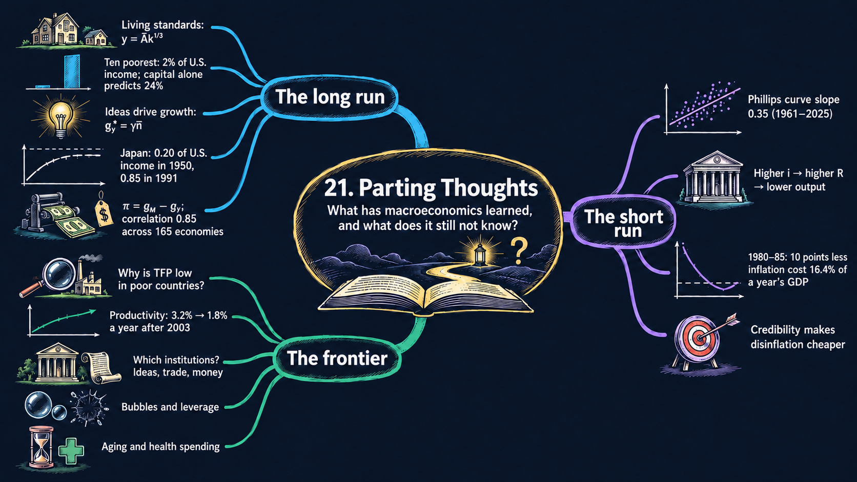



Learning goals
The textbook ends by looking back at what macroeconomics has learned and ahead at what it still does not know. By the end of this notebook you will be able to:
- state the five main lessons of the book in your own words: living standards, transition dynamics, the classical dichotomy, the short-run Phillips curve trade-off and central-bank credibility;
- restate the key results of every model in the book and derive them step by step from their building blocks: development accounting, the Solow steady state, long-run growth from ideas, the natural rate of unemployment, the quantity theory, the IS, Phillips and AD curves, the path of inflation in a disinflation, the Euler equation, the user cost of capital and the government’s budget constraint;
- read the comparative statics of each model: which parameter moves which result, in which direction and by how much, and check the headline results with short Python simulations;
- find the model and the figure in earlier notebooks where each lesson was built;
- recompute a key number for each lesson from real data, such as Japan’s catch-up growth or the slope of the U.S. Phillips curve, and compare Japan’s catch-up with any of 167 other economies in a country picker;
- name a few open questions at the frontier of research, such as the productivity slowdown after 2003;
- reuse the Python you have learned:
read_csv, filtering rows,merge,pivot, short functions andnp.polyfit.
Model overview
For twenty chapters we have followed Islandia, our small imaginary island country. We watched its tools pile up and wear out and new ideas spread, and we followed its jobs, money, booms and slumps, its households, Harbor Boatworks, its Treasury and its trade with Mainland. This overview builds no new model. It lays the book’s models side by side, so that we can look back at Islandia’s whole story before five lessons test it with data.
NoteThe big idea
The question. Looking back at the whole book, what makes an economy like Islandia rich or poor, what makes it grow, and what causes its booms and slumps?
The answer in one sentence. Over decades, real forces (tools, skills and above all ideas) set the level and the growth of income while money sets only prices; over a year or two, sticky inflation lets demand and the central bank move output.
What goes in and what comes out. Each block takes the parameters of its own chapters and gives back its headline results, numbered (1) to (20), which the code and the five lessons reuse.
Road map.
- Long run: the production model.
- Long run: the Solow model.
- Long run: ideas, the Romer model and the combined model.
- Long run: unemployment, money and inflation.
- Short run: the IS curve, the MP curve and the Phillips curve.
- Short run: stabilization and the AS/AD framework.
- Behind the curves: consumption and investment.
- The government and the open economy.
- Model in code: each headline result checked a second way in Python.
Notation. As everywhere in the book, a bar marks a parameter, a number taken as given; letters without a bar are endogenous variables, which the models determine.
| Symbol | Meaning | Type |
|---|---|---|
| \(Y, K, L\) | output, capital and labor | endogenous |
| \(y, k\) | output and capital per person | endogenous |
| \(A_t, u, \pi, i, R\) | ideas, unemployment, inflation, nominal and real interest rates | endogenous |
| \(\bar{A}, \bar{s}, \bar{d}, \bar{n}\) | TFP, investment rate, depreciation rate, population growth | parameters |
| \(y^*\) | a star marks a long-run value, such as a steady state | notation |
| \(\tilde{Y}_t\) | a tilde marks short-run output, the percent gap between actual and potential output | notation |
| \(g_x\), \(\Delta x_{t+1}\) | the growth rate of \(x\), and its change \(x_{t+1} - x_t\) | notation |
Long run: the production model
Back to Chapter 4.
Building blocks
Islandia makes one good with capital \(K\), its tools, and labor \(L\). Total factor productivity \(\bar{A}\), how well the islanders combine the two, is a parameter:
\[Y = F(K, L) = \bar{A}K^{1/3}L^{2/3}.\]
Firms such as Harbor Boatworks rent capital at the price \(r\) and hire workers at the wage \(w\) to maximize profit \(\Pi = F(K,L) - rK - wL\). The inputs are given, \(K = \bar{K}\) and \(L = \bar{L}\), so the prices adjust until firms want exactly those amounts.
Key results
Factor prices. Profit peaks where one more unit of an input adds just as much output as it costs (Appendix C.8). That extra output is the marginal product, the derivative of \(F\) with respect to the input. The power rule (Appendix C.7) brings the exponent down and lowers it by one:
\[MPK = \tfrac{1}{3}\bar{A}K^{1/3-1}L^{2/3} = \tfrac{1}{3}\cdot\frac{\bar{A}K^{1/3}L^{2/3}}{K} = \tfrac{1}{3}\cdot\frac{Y}{K}, \qquad MPL = \tfrac{2}{3}\cdot\frac{Y}{L}.\]
So \(r^* = \frac{1}{3}Y^*/\bar{K}\) and \(w^* = \frac{2}{3}Y^*/\bar{L}\). Multiply each price by its input to get the factor shares: capital receives \(r^*\bar{K}/Y^* = 1/3\) of output and labor receives \(w^*\bar{L}/Y^* = 2/3\). The shares sum to one, so profit is zero: constant returns to scale at work.
Output per person. Divide the production function by \(\bar{L}\), use \(\bar{L}^{2/3}/\bar{L} = \bar{L}^{-1/3}\) (Appendix C.3), and write capital per person as \(\bar{k} \equiv \bar{K}/\bar{L}\). The result is equation (1) in the box below.
Comparing two economies. Write equation (1) for economy 1 and for economy 2, then divide the first by the second. The result is equation (2).
ImportantKey result: output per person and development accounting
\[y^* = \bar{A}\bar{k}^{1/3}. \tag{1}\]
\[\frac{y_1^*}{y_2^*} = \frac{\bar{A}_1}{\bar{A}_2}\times\left(\frac{\bar{k}_1}{\bar{k}_2}\right)^{1/3}. \tag{2}\]
In equation (2), the second factor is the relative income that capital alone predicts; the first is relative TFP.
Islandia in numbers. Compare young Islandia (economy 1) with today’s (economy 2), as in Check 1 of the code: with half of today’s TFP and \(1/27\) of its tools per person, \(y_1^*/y_2^* = 0.5 \times (1/27)^{1/3} \approx 0.167\), about a sixth.
In the data, economy 2 is the United States (for Islandia, the richer Mainland). We can measure \(y^*\) and \(\bar{k}\), but not \(\bar{A}\), so TFP is found as the part that capital leaves unexplained, \(\bar{A} = y^*/\bar{k}^{1/3}\). This is development accounting, and Lesson 1 applies it to the world.
TipIn words: why tools cannot explain big gaps
Hand an islander from young Islandia today’s tools, and only part of the income gap closes. With the exponent \(1/3\), being ten times richer through tools alone takes \(10^3 = 1{,}000\) times as many tools. These strong diminishing returns mean that large gaps come mostly from know-how, TFP.
Comparative statics. In logs (Appendix C.4), \(\ln y^* = \ln\bar{A} + \frac{1}{3}\ln\bar{k}\). One percent more TFP gives 1 percent more output per person; one percent more capital per person gives only a third of a percent more. The wage \(w^* = \frac{2}{3}y^*\) moves in proportion to output per person.
Tools raise income, but with strong diminishing returns, so large income gaps point mostly to gaps in productivity.
NoteCheck your understanding
1. Young Islandia had the same TFP as today but only one eighth of today’s tools per person. How many times richer is Islandia today?
Answer
By equation (2) with equal TFP, \(y_{\text{today}}^*/y_{\text{young}}^* = 8^{1/3} = 2\). Eight times the tools buy only twice the income.
2. Why is TFP measured as a residual?
Answer
We observe income and tools per person, but not know-how. Solving equation (1) for it, \(\bar{A} = y^*/\bar{k}^{1/3}\), assigns to TFP whatever tools leave unexplained.
Long run: the Solow model
Back to Chapter 5.
Building blocks
Now Islandia builds its own tools: capital is endogenous. Five equations hold in every year \(t\):
| Equation | Meaning |
|---|---|
| \(Y_t = \bar{A}K_t^{1/3}L_t^{2/3}\) | production |
| \(C_t + I_t = Y_t\) | output is eaten or invested |
| \(\Delta K_{t+1} = I_t - \bar{d}K_t\) | tools grow by investment minus the tools that break |
| \(L_t = \bar{L}\) | a constant labor force |
| \(I_t = \bar{s}Y_t\) | a constant share \(\bar{s}\) of output is invested |
Key results
One equation for capital. Substitute \(I_t = \bar{s}Y_t\) into the accumulation equation and divide every term by \(\bar{L}\). With \(k_t \equiv K_t/\bar{L}\) and \(y_t = \bar{A}k_t^{1/3}\), as in equation (1):
\[\Delta k_{t+1} = \bar{s}\bar{A}k_t^{1/3} - \bar{d}k_t.\]
The terms are new tools and broken tools per person.
The steady state. Capital stops changing when the two terms are equal. Divide \(\bar{s}\bar{A}(k^*)^{1/3} = \bar{d}k^*\) by \(\bar{d}(k^*)^{1/3}\) to get \((k^*)^{2/3} = \bar{s}\bar{A}/\bar{d}\), then raise both sides to the power \(3/2\): \(k^* = (\bar{s}\bar{A}/\bar{d})^{3/2}\). Putting \(k^*\) into the production function multiplies the exponents, \(\frac{3}{2}\times\frac{1}{3} = \frac{1}{2}\), so \(y^* = \bar{A}(\bar{s}\bar{A}/\bar{d})^{1/2}\). Collecting the powers of \(\bar{A}\) gives equation (3) below.
Transition dynamics. Divide the capital equation by \(k_t\) to get the growth rate of capital per person, \(g_{k,t} = \bar{s}\bar{A}k_t^{-2/3} - \bar{d}\). The steady state says \(\bar{s}\bar{A} = \bar{d}(k^*)^{2/3}\). Substituting it leaves equation (4), which depends only on how far the economy is from its steady state.
ImportantKey result: the Solow steady state and transition dynamics
\[y^* = \left(\frac{\bar{s}}{\bar{d}}\right)^{1/2}\bar{A}^{3/2}. \tag{3}\]
\[g_{k,t} = \bar{d}\left[\left(\frac{k^*}{k_t}\right)^{2/3} - 1\right]. \tag{4}\]
Islandia in numbers. With \(\bar{s} = 0.25\), \(\bar{d} = 0.05\) and \(\bar{A} = 1\) (Check 2 of the code), \(\bar{s}/\bar{d} = 5\), so \(y^* = 5^{1/2} \approx 2.24\). With half its steady-state tools, Islandia adds \(0.05\times(2^{2/3}-1) \approx 2.9\%\) to its capital per person in a year.
By the power rule for growth rates (Appendix C.5), output per person grows about a third as fast, \(g_{y,t} \approx \frac{1}{3}g_{k,t}\). An economy below its steady state grows, faster the larger the gap; an economy above it shrinks. This is the simplest form of the principle of transition dynamics behind Lesson 2.
TipIn words: the race between new and broken tools
With few tools, each new tool adds a lot of output, so new tools outnumber broken ones. As tools pile up, each adds less, while breakage keeps pace. The race ends in a tie at the steady state. After the storm destroyed part of Islandia’s tools, the island rebuilt fast at first, then more slowly.
Comparative statics. In logs, \(\ln y^* = \frac{1}{2}\ln\bar{s} - \frac{1}{2}\ln\bar{d} + \frac{3}{2}\ln\bar{A}\):
| A 1% rise in … | changes \(y^*\) by | why |
|---|---|---|
| investment rate \(\bar{s}\) | \(+0.5\%\) | more capital, but with diminishing returns |
| depreciation rate \(\bar{d}\) | \(-0.5\%\) | more of each year’s investment only replaces worn-out capital |
| TFP \(\bar{A}\) | \(+1.5\%\) | a direct effect of 1, plus 1/2 through the extra capital it pays for |
No growth in the long run. At the steady state \(k^*\) and \(y^*\) are constant. Each extra tool adds less output than the one before but breaks just as often, so building tools alone cannot keep income per person rising. With population growth at rate \(\bar{n}\), every step goes through with \(\bar{n} + \bar{d}\) in place of \(\bar{d}\).
Building tools raises income only until new tools just replace broken ones; after that, tools alone bring no growth.
NoteCheck your understanding
1. Islandia doubles its investment rate from 0.25 to 0.5, with \(\bar{d} = 0.05\) and \(\bar{A} = 1\). What is the new \(y^*\), and by what percentage does it rise?
Answer
Now \(\bar{s}/\bar{d} = 10\), so equation (3) gives \(y^* = 10^{1/2} \approx 3.16\), up from about 2.24. That is a rise of about 41 percent: doubling the investment rate multiplies income by only \(2^{1/2}\).
2. The storm destroyed part of Islandia’s tools. Does its long-run income change? Why does its growth slow down over the following years?
Answer
No: the starting stock of tools is not in equation (3). By equation (4), growth fades as \(k_t\) approaches \(k^*\) and the ratio \(k^*/k_t\) falls toward one.
Long run: ideas, the Romer model and the combined model
Back to Chapter 6.
Building blocks
The Romer model explains where TFP comes from. Islandia’s population \(N_t\) splits between making goods (\(L_{yt}\)) and doing research (\(L_{at}\)), and \(A_t\) is the stock of ideas:
| Equation | Meaning |
|---|---|
| \(Y_t = A_t^{\gamma}L_{yt}\) | goods are made with ideas and workers |
| \(\Delta A_{t+1} = \bar{z}L_{at}\) | each researcher adds \(\bar{z}\) new ideas a year |
| \(L_{yt} + L_{at} = N_t\) | everyone works in one of the two sectors |
| \(\Delta N_{t+1}/N_t = \bar{n}\) | the population grows at rate \(\bar{n}\) |
| \(L_{at} = \bar{\ell}N_t\) | a constant share \(\bar{\ell}\) of people do research |
The parameter \(\gamma > 0\) measures how strongly ideas raise output. Ideas are nonrival: every worker can use the whole stock \(A_t\) at once, so doubling ideas and workers multiplies output by \(2^{1+\gamma}\): increasing returns.
Key results
Income per person depends on the total stock of ideas. With \(L_{yt} = (1-\bar{\ell})N_t\), divide output by \(N_t\); this gives equation (5) in the box below.
Ideas grow as fast as the population. Divide the idea equation by \(A_t\): \(g_{At} = \bar{z}L_{at}/A_t\). This growth rate stays constant only if the numerator and the denominator grow at the same rate (the ratio rule of Appendix C.5). Researchers \(L_{at} = \bar{\ell}N_t\) grow at \(\bar{n}\), so in the long run \(g_A^* = \bar{n}\). The economy is pulled there: if ideas grew faster than \(\bar{n}\), the ratio \(L_{at}/A_t\) would fall and drag \(g_{At}\) down, and the reverse if they grew more slowly. Solving \(\bar{n} = \bar{z}\bar{\ell}N_t/A_t\) for the stock gives \(A_t^* = \bar{z}\bar{\ell}N_t/\bar{n}\): more researchers support a larger stock of knowledge.
Long-run growth. Put \(A_t^*\) into equation (5): \(y_t^* = (\bar{z}\bar{\ell}N_t/\bar{n})^{\gamma}(1-\bar{\ell})\). Only \(N_t\) changes over time, and the growth rate of a power is the power times the growth rate. This gives equation (6).
ImportantKey result: the Romer model
\[y_t \equiv \frac{Y_t}{N_t} = A_t^{\gamma}(1-\bar{\ell}). \tag{5}\]
\[g_y^* = \gamma\bar{n}. \tag{6}\]
Islandia in numbers. With \(\gamma = 0.5\) and \(\bar{n} = 0.02\) (Check 3 of the code), \(g_y^* = 0.5 \times 0.02 = 0.01\), or 1 percent a year.
TipIn words: ideas are shared by everyone at once
Islandia’s researchers keep adding blueprints to a library that never wears out, and every islander can use the whole library at once. A growing population means more researchers, so new blueprints, and income per person, keep coming.
Comparative statics. A higher research productivity \(\bar{z}\) or research share \(\bar{\ell}\) lifts the level of income per person on the long-run path, but not its long-run growth rate, which depends only on \(\gamma\) and \(\bar{n}\). A higher \(\bar{\ell}\) also costs something today: fewer people make goods, the factor \(1-\bar{\ell}\). (In Romer’s original version, \(\Delta A_{t+1}/A_t = \bar{z}L_{at}\), the same changes raise the growth rate itself.)
The combined Solow–Romer model. Now let ideas and tools work together: \(Y_t = A_t^{\gamma}K_t^{1/3}L_{yt}^{2/3}\), with \(\Delta K_{t+1} = \bar{s}Y_t - \bar{d}K_t\) and ideas, people and researchers as above. Per person, \(y_t = A_t^{\gamma}k_t^{1/3}(1-\bar{\ell})^{2/3}\), and the growth rules for products and powers give
\[g_{yt} = \gamma g_{At} + \tfrac{1}{3}g_{kt}.\]
On a balanced growth path the capital-output ratio is constant, so capital and output grow at the same rate, \(g_k^* = g_y^*\). Substituting this and \(g_A^* = \bar{n}\) gives \(g_y^* = \gamma\bar{n} + \frac{1}{3}g_y^*\), so \(\frac{2}{3}g_y^* = \gamma\bar{n}\): equation (7) below. Growth beats the Romer model alone because part of the output that ideas add is invested in tools.
The level of the path. Divide the capital equation by \(K_t\): \(g_{Kt} = \bar{s}Y_t/K_t - \bar{d}\). On the balanced growth path \(g_K^* = g_Y^*\), so \(K_t^*/Y_t^* = \bar{s}/(g_Y^* + \bar{d})\), where \(g_Y^* = g_y^* + \bar{n}\) is the growth rate of total output. Write the production function as \(Y_t = A_t^{\gamma}(K_t/Y_t)^{1/3}Y_t^{1/3}L_{yt}^{2/3}\), move \(Y_t^{1/3}\) to the left to get \(Y_t^{2/3}\), and raise both sides to the power \(3/2\): \(Y_t = A_t^{3\gamma/2}(K_t/Y_t)^{1/2}L_{yt}\). Dividing by \(N_t\) gives equation (8). Investment, depreciation and the research share set the level of the path, as in the Solow model; ideas set its slope. (With \(\gamma = 1\) the exponent on \(A_t^*\) is \(3/2\), as in equation (3).)
Transition dynamics in the combined model. Subtract the balanced-growth version of the growth equation, \(g_y^* = \gamma\bar{n} + \frac{1}{3}g_y^*\), from the general one, \(g_{yt} = \gamma\bar{n} + \frac{1}{3}g_{kt}\). This gives equation (9), where the growth of capital per person comes from dividing the capital equation by \(K_t\) and subtracting \(\bar{n}\).
ImportantKey result: the combined Solow–Romer model
\[g_y^* = \tfrac{3}{2}\gamma\bar{n}. \tag{7}\]
\[y_t^* = \left(\frac{\bar{s}}{g_Y^*+\bar{d}}\right)^{1/2}A_t^{*\,3\gamma/2}(1-\bar{\ell}). \tag{8}\]
\[g_{yt} - g_y^* = \tfrac{1}{3}\left(g_{kt} - g_y^*\right), \qquad g_{kt} = \bar{s}\frac{Y_t}{K_t} - \bar{d} - \bar{n}. \tag{9}\]
Islandia in numbers. Add \(\bar{s} = 0.2\) and \(\bar{d} = 0.05\) (Check 4 of the code). Then \(g_y^* = 1.5 \times 0.5 \times 0.02 = 0.015\), or 1.5 percent a year, total output grows at \(0.015 + 0.02 = 0.035\), and the path’s capital-output ratio is \(0.2/(0.035 + 0.05) \approx 2.35\).
With less capital per unit of output than on the path, \(Y_t/K_t\) is high, so capital and income per person grow faster than \(g_y^*\) until the gap closes. Countries below their own path grow fast, those above it slowly: the version of transition dynamics that Lesson 2 checks with Japan’s catch-up.
Ideas, which everyone can use at once, are the source of lasting growth; tools amplify that growth but cannot sustain it alone.
NoteCheck your understanding
1. In the combined model with \(\gamma = 0.5\), Islandia’s population growth rises from 2 to 3 percent a year. What is the new long-run growth rate of income per person?
Answer
By equation (7), \(g_y^* = 1.5 \times 0.5 \times 0.03 = 0.0225\), or 2.25 percent a year, up from 1.5 percent. More people means more researchers and so more new ideas.
2. Islandia moves more people into research, a higher \(\bar{\ell}\). Does its long-run growth rate change?
Answer
No: by equation (7) it depends only on \(\gamma\) and \(\bar{n}\). More ideas raise the level of the path, but fewer islanders make goods, the factor \(1-\bar{\ell}\) in equation (8).
Long run: unemployment, money and inflation
Back to Chapter 7 and Chapter 8.
Building blocks
Labor market flows. Islandia’s labor force \(\bar{L}\) is split into employed and unemployed islanders, \(E_t + U_t = \bar{L}\). Each year a share \(\bar{s}\) of the employed lose their jobs (here \(\bar{s}\) is the job-losing rate, not the investment rate) and a share \(\bar{f}\) of the unemployed find one:
\[\Delta U_{t+1} = \bar{s}E_t - \bar{f}U_t.\]
The quantity theory of money. Money times its velocity, the number of times each unit of money is spent in a year, equals nominal GDP: \(M_tV_t = P_tY_t\). Velocity is constant, \(V_t = \bar{V}\); real GDP \(\bar{Y}_t\) is set by the real side of the economy (the models above); and the central bank, the Bank of Islandia, chooses the money supply \(\bar{M}_t\).
Interest rates and the government’s sources of funds. The nominal interest rate \(i\) is the real rate \(R\) plus inflation \(\pi\). The government pays for its spending \(G\) with taxes, new borrowing or new money, \(G = T + \Delta B + \Delta M\).
Key results
The natural rate of unemployment. Unemployment is steady when as many people find jobs as lose them, \(\bar{s}E^* = \bar{f}U^*\). Replace \(E^*\) with \(\bar{L} - U^*\), multiply out and collect the \(U^*\) terms: \(\bar{s}\bar{L} = (\bar{s}+\bar{f})U^*\). Dividing by \(\bar{L}\) gives equation (10) below.
The price level and inflation. Solving the quantity equation for prices gives \(P_t^* = \bar{M}_t\bar{V}/\bar{Y}_t\). The growth rate of a product is the sum of the growth rates (Appendix C.5), so \(\bar{g}_M + \bar{g}_V = g_P + \bar{g}_Y\). Velocity is constant, \(\bar{g}_V = 0\), and inflation is the growth rate of the price level, \(\pi = g_P\). This gives equation (11).
The Fisher equation. Writing the link between the two interest rates as an equation gives (12).
ImportantKey result: the natural rate, the quantity theory and the Fisher equation
\[u^* \equiv \frac{U^*}{\bar{L}} = \frac{\bar{s}}{\bar{s}+\bar{f}}. \tag{10}\]
\[\pi^* = \bar{g}_M - \bar{g}_Y. \tag{11}\]
\[i = R + \pi. \tag{12}\]
Islandia in numbers. With job-losing and job-finding rates of 0.02 and 0.3 (Check 5 of the code), \(u^* = 0.02/0.32 = 6.25\) percent. With money growing 7 percent a year and real GDP 3 percent, inflation is 4 percent.
Unemployment is high where jobs end often (high \(\bar{s}\)) or take long to find (low \(\bar{f}\)). Institutions such as firing costs and unemployment insurance work through these two rates, not through money.
One more point of money growth means one more point of inflation; one more point of real growth means one point less. Real GDP was settled before money entered the story, so money changes prices but not real output: the classical dichotomy.
Lenders want compensation for the purchasing power inflation takes away. In the long run \(R\) is set by the marginal product of capital, so inflation passes one for one into nominal rates.
Where high inflation comes from. Rearranged, the sources of funds give \(\Delta M = G - T - \Delta B\): a government with a large deficit that cannot borrow prints money, and equation (11) turns it into inflation.
TipIn words: real forces and the price tag
Each year some islanders lose jobs at Harbor Boatworks and elsewhere, and some are hired. Unemployment settles where the two flows match, whatever money does. Money sets only the price tag: if the Bank of Islandia adds money faster than the island adds goods, prices rise.
In the long run, real forces set jobs and output, while money sets only prices and the inflation rate.
NoteCheck your understanding
1. Jobs on Islandia become harder to find: the job-finding rate falls from 0.3 to 0.18, with a job-losing rate of 0.02. What is the new natural rate of unemployment?
Answer
By equation (10), \(u^* = 0.02/(0.02 + 0.18) = 0.1\), or 10 percent, up from 6.25 percent.
2. The Bank of Islandia raises money growth from 7 to 9 percent a year, and real growth stays at 3 percent. What happens in the long run to inflation and to the nominal interest rate?
Answer
By equation (11), inflation rises to 6 percent. The real rate does not change (the classical dichotomy), so by equation (12) the nominal rate rises by two points too.
Short run: the IS curve, the MP curve and the Phillips curve
Back to Chapter 9, Chapter 11 and Chapter 12.
Building blocks
Short-run output. Potential output \(\bar{Y}_t\) is the long-run path of the models above, and short-run output is the percent gap \(\tilde{Y}_t \equiv (Y_t - \bar{Y}_t)/\bar{Y}_t\). Okun’s law links it to unemployment: \(u_t - \bar{u} = -\frac{1}{2}\tilde{Y}_t\).
Demand. Output is spent on \(Y_t = C_t + I_t + G_t + EX_t - IM_t\). Consumption, government purchases, exports and imports are constant shares of potential output, \(C_t = \bar{a}_c\bar{Y}_t\), \(G_t = \bar{a}_g\bar{Y}_t\), \(EX_t = \bar{a}_{ex}\bar{Y}_t\) and \(IM_t = \bar{a}_{im}\bar{Y}_t\). Investment falls when the real interest rate \(R_t\) rises above the marginal product of capital \(\bar{r}\): \(I_t/\bar{Y}_t = \bar{a}_i - \bar{b}(R_t - \bar{r})\).
Monetary policy (the MP curve). The central bank sets the nominal interest rate \(i_t\). Inflation is sticky, so it barely moves in the short run, and by the Fisher equation (12) the real rate \(R_t = i_t - \pi_t\) moves with \(i_t\): in effect, the central bank chooses \(R_t\).
Price setting (the Phillips curve). Inflation equals expected inflation, plus a term for demand, plus a price shock \(\bar{o}\): \(\pi_t = \pi_t^e + \bar{\nu}\tilde{Y}_t + \bar{o}\). Expectations are adaptive: people expect last year’s inflation, \(\pi_t^e = \pi_{t-1}\).
Key results
The IS curve. Divide the spending identity by \(\bar{Y}_t\) and use the shares: \(Y_t/\bar{Y}_t = \bar{a}_c + \bar{a}_i - \bar{b}(R_t - \bar{r}) + \bar{a}_g + \bar{a}_{ex} - \bar{a}_{im}\). Subtract 1 from both sides; the left side becomes \((Y_t - \bar{Y}_t)/\bar{Y}_t = \tilde{Y}_t\), and the result is equation (13) below.
The Phillips curve. Substitute adaptive expectations into the price equation and subtract \(\pi_{t-1}\) from both sides. The result is equation (14).
ImportantKey result: the IS curve and the Phillips curve
\[\tilde{Y}_t = \bar{a} - \bar{b}(R_t - \bar{r}), \qquad \bar{a} \equiv \bar{a}_c + \bar{a}_i + \bar{a}_g + \bar{a}_{ex} - \bar{a}_{im} - 1. \tag{13}\]
\[\Delta\pi_t = \bar{\nu}\tilde{Y}_t + \bar{o}. \tag{14}\]
Islandia in numbers. With \(\bar{a} = 0\), \(\bar{b} = 2\) and \(\bar{r} = 2\) percent (Check 6 of the code), a real rate of 5 percent gives \(\tilde{Y}_t = -2 \times 3 = -6\) percent. With \(\bar{\nu} = 0.5\) (Check 7), inflation then falls by \(0.5 \times 6 = 3\) points.
The demand shock \(\bar{a}\) collects everything else that shifts spending; it is zero in the long run, when also \(R_t = \bar{r}\), so that \(\tilde{Y}_t = 0\). If consumption also rises with current output, \(C_t/\bar{Y}_t = \bar{a}_c + \bar{x}\tilde{Y}_t\), the same steps give \(\tilde{Y}_t = \bar{a} + \bar{x}\tilde{Y}_t - \bar{b}(R_t - \bar{r})\), and solving for \(\tilde{Y}_t\) multiplies the right side of equation (13) by the multiplier \(1/(1-\bar{x})\). By equation (14), inflation rises in a boom and falls in a slump.
TipIn words: a rate hike on Islandia
The Bank of Islandia raises its rate. Inflation hardly moves, so the real rate climbs too. Borrowing now costs Harbor Boatworks more than a new boat shed would earn, so it waits. Output falls below potential, and with slack, firms raise prices more slowly.
The chain of monetary policy. Line the three curves up: a higher \(i_t\) raises \(R_t\) (MP curve), which lowers \(\tilde{Y}_t\) (IS curve), which lowers the change in inflation (Phillips curve) and raises unemployment (Okun’s law).
| A change of +1 in … | moves … | by |
|---|---|---|
| the real interest rate \(R_t\) (points) | short-run output \(\tilde{Y}_t\) | \(-\bar{b}\) percent |
| the demand shock \(\bar{a}\) | short-run output \(\tilde{Y}_t\) | \(+1\) percent (the IS curve shifts right) |
| short-run output \(\tilde{Y}_t\) (percent) | the change in inflation \(\Delta\pi_t\) | \(+\bar{\nu}\) points |
| short-run output \(\tilde{Y}_t\) (percent) | unemployment \(u_t\) | \(-\frac{1}{2}\) point |
| the price shock \(\bar{o}\) | the change in inflation \(\Delta\pi_t\) | \(+1\) point (the Phillips curve shifts up) |
Because inflation is sticky, the central bank moves the real interest rate, and with it spending, output and next year’s inflation.
NoteCheck your understanding
1. With \(\bar{a} = 0\), \(\bar{b} = 2\), \(\bar{r} = 2\) percent and \(\bar{\nu} = 0.5\), the Bank of Islandia sets a real rate of 1 percent. What are short-run output, the change in inflation and the change in unemployment?
Answer
By equation (13), \(\tilde{Y}_t = -2 \times (1 - 2) = +2\) percent. By equation (14), inflation rises by \(0.5 \times 2 = 1\) point. By Okun’s law, unemployment is 1 point below its natural rate.
2. A jump in oil prices hits Islandia, \(\bar{o} > 0\). Which curve moves, and what happens to inflation if the Bank of Islandia keeps the real rate unchanged?
Answer
The Phillips curve (14) shifts up; the IS curve (13) stays. With \(R_t\) unchanged, output does not move and inflation rises by \(\bar{o}\).
Short run: stabilization and the AS/AD framework
Back to Chapter 13 and Chapter 14.
Building blocks
Now the central bank follows a monetary policy rule: it raises the real rate above \(\bar{r}\) when inflation is above its target \(\bar{\pi}\),
\[R_t - \bar{r} = \bar{m}(\pi_t - \bar{\pi}), \qquad \bar{m} > 0.\]
The IS curve (13) and the Phillips curve (14) stay as they are. Written as \(\pi_t = \pi_{t-1} + \bar{\nu}\tilde{Y}_t + \bar{o}\), the Phillips curve is the aggregate supply (AS) curve. In a financial crisis firms borrow at the policy rate plus a risk premium, \(R_t = R_t^{ff} + \bar{f}\).
Key results
The AD curve. Replace \(R_t - \bar{r}\) in the IS curve by the policy rule; this gives equation (15) below. The curve slopes down: when inflation is high, the central bank raises the real rate, and spending falls.
The steady state. With no shocks (\(\bar{a} = \bar{o} = 0\)), AD gives \(\tilde{Y}_t = 0\) only at \(\pi_t = \bar{\pi}\), and AS keeps inflation there: output at potential, inflation on target.
The path of inflation. Put the AD curve into the AS curve: \(\pi_t = \pi_{t-1} + \bar{\nu}\bar{a} - \bar{\nu}\bar{b}\bar{m}(\pi_t - \bar{\pi}) + \bar{o}\). Subtract \(\bar{\pi}\) from both sides and move the \(\pi_t\) term to the left: \((1 + \bar{\nu}\bar{b}\bar{m})(\pi_t - \bar{\pi}) = (\pi_{t-1} - \bar{\pi}) + \bar{\nu}\bar{a} + \bar{o}\). Without shocks, dividing by \(1 + \bar{\nu}\bar{b}\bar{m}\) gives equation (16).
ImportantKey result: the AD curve and the path of inflation
\[\tilde{Y}_t = \bar{a} - \bar{b}\bar{m}(\pi_t - \bar{\pi}). \tag{15}\]
\[\pi_t - \bar{\pi} = \frac{\pi_{t-1} - \bar{\pi}}{1 + \bar{\nu}\bar{b}\bar{m}}. \tag{16}\]
Islandia in numbers. With \(\bar{\nu} = 0.5\), \(\bar{b} = 1\) and \(\bar{m} = 0.5\) (Check 7 of the code), the factor is \(1 + \bar{\nu}\bar{b}\bar{m} = 1.25\). When the Bank of Islandia cuts its target from 6 to 2 percent, inflation falls to \(2 + 4/1.25 = 5.2\) percent in the first year.
By the Fisher equation (12), the rule sets the nominal rate at \(i_t = \bar{r} + \pi_t + \bar{m}(\pi_t - \bar{\pi})\), so each point of inflation raises the nominal rate by \(1 + \bar{m}\) points, more than one for one. Equation (16) is a first-order difference equation (Appendix C.10), and output follows from AD, \(\tilde{Y}_t = -\bar{b}\bar{m}(\pi_t - \bar{\pi})\). A central bank that reacts more strongly (a larger \(\bar{m}\)) closes the gap faster, with a deeper recession at the start.
The cost of a disinflation. Lowering the target \(\bar{\pi}\) leaves last year’s inflation above the new target, so equation (16) brings inflation down through a recession. Adding the AS curve up over all the years of the adjustment, the changes in inflation sum to the total fall, \(\pi_{\text{start}} - \bar{\pi} = -\bar{\nu}\sum_t \tilde{Y}_t\). So the output lost per point of disinflation, the sacrifice ratio, is \(1/\bar{\nu}\) under adaptive expectations, however fast the central bank moves. If instead price setters believe the new target, expected inflation drops straight to it, \(\pi_t^e = \bar{\pi}\), and inflation can fall with \(\tilde{Y}_t = 0\): the gain from credibility in Lesson 5.
Financial crises. Write the borrowing rate gap as \(R_t - \bar{r} = (R_t^{ff} - \bar{r}) + \bar{f}\) and let the central bank set the policy-rate gap by its rule. The AD curve becomes \(\tilde{Y}_t = (\bar{a} - \bar{b}\bar{f}) - \bar{b}\bar{m}(\pi_t - \bar{\pi})\): a higher risk premium works like a negative demand shock of size \(\bar{b}\bar{f}\), which the central bank can offset only while it can still cut \(R_t^{ff}\). Leverage makes banks fragile: a fall in asset values of one over the leverage ratio wipes out all equity.
TipIn words: the Bank of Islandia brings inflation down
While inflation is above target, the Bank of Islandia keeps the real rate high, islanders spend less, and the slack pulls inflation a fixed share of the way back each year. If islanders believe a lower target, they cut their price plans at once, and the slump can be much milder.
A rule that leans against inflation brings it back to target, and credibility makes the trip cheaper in lost output.
NoteCheck your understanding
1. Continue the disinflation from 6 to 2 percent with \(\bar{\nu} = 0.5\), \(\bar{b} = 1\) and \(\bar{m} = 0.5\). What are inflation and short-run output in the second year?
Answer
The first-year gap is \(5.2 - 2 = 3.2\) points. By equation (16), the second-year gap is \(3.2/1.25 = 2.56\), so inflation is 4.56 percent. By equation (15) with \(\bar{a} = 0\), \(\tilde{Y}_t = -1 \times 0.5 \times 2.56 = -1.28\) percent.
2. Would a tougher Bank of Islandia, with a larger \(\bar{m}\), reduce the total output lost in this disinflation if expectations are adaptive?
Answer
No. Summing the AS curve, the total loss is the fall in inflation over \(\bar{\nu}\), \(4/0.5\): 8 percent of a year’s potential output, whatever \(\bar{m}\) is. A larger \(\bar{m}\) only packs it into fewer, deeper years.
Behind the curves: consumption and investment
Back to Chapter 16 and Chapter 17.
Building blocks
A household over two periods. An islander earns \(y_{\text{today}}\) and \(y_{\text{future}}\), can save or borrow \(f_{\text{future}}\) at the real rate \(R\), and starts with no assets. Today \(c_{\text{today}} + f_{\text{future}} = y_{\text{today}}\); in the future \(c_{\text{future}} = y_{\text{future}} + (1+R)f_{\text{future}}\). The household chooses consumption to maximize \(U = u(c_{\text{today}}) + \beta u(c_{\text{future}})\), where \(\beta\) discounts the future.
A firm deciding whether to buy capital. One unit of capital costs \(p_k\). Put in the bank, the money earns \(R\,p_k\). Used as capital, it earns its marginal product, loses \(\bar{d}p_k\) to wear and tear, and gains (or loses) \(\Delta p_k\) in price. The firm buys capital until the two returns are equal: \(R\,p_k = MPK - \bar{d}p_k + \Delta p_k\).
Key results
The lifetime budget constraint. From today’s budget, \(f_{\text{future}} = y_{\text{today}} - c_{\text{today}}\). Put it into the future budget, divide by \(1+R\) and move consumption to the left: \(c_{\text{today}} + c_{\text{future}}/(1+R) = y_{\text{today}} + y_{\text{future}}/(1+R) \equiv \bar{X}\). The present value of consumption equals the present value of income, lifetime wealth (Appendix C.12).
The Euler equation. Giving up one unit today costs \(u'(c_{\text{today}})\) in utility. Saved, it becomes \(1+R\) units in the future, each worth \(\beta u'(c_{\text{future}})\) today. At the best plan the two are equal, \(u'(c_{\text{today}}) = \beta(1+R)u'(c_{\text{future}})\). With log utility, \(u'(c) = 1/c\), which gives equation (17) below. Substitute \(c_{\text{future}} = \beta(1+R)c_{\text{today}}\) into the lifetime budget: the \((1+R)\) cancels and \(c_{\text{today}}(1+\beta) = \bar{X}\), so \(c_{\text{today}} = \bar{X}/(1+\beta)\). With \(\beta = 1\) the household consumes half of its lifetime wealth today.
The user cost of capital. Divide the firm’s condition by \(p_k\) and solve for the marginal product. This gives equation (18).
ImportantKey result: the Euler equation and the user cost of capital
\[\frac{c_{\text{future}}}{c_{\text{today}}} = \beta(1+R). \tag{17}\]
\[MPK = \underbrace{R + \bar{d} - \frac{\Delta p_k}{p_k}}_{\text{user cost } uc}. \tag{18}\]
Islandia in numbers. With \(\beta = 0.95\) and \(R = 0.04\) (Check 8 of the code), \(c_{\text{future}}/c_{\text{today}} = 0.95 \times 1.04 = 0.988\). With \(R = 0.02\), \(\bar{d} = 0.08\) and no price change, the user cost is 0.10 and the desired capital-output ratio is \(1/(3 \times 0.10) \approx 3.33\).
Implications. Consumption depends on lifetime wealth (the permanent-income hypothesis), so a temporary change in income moves it little. A tax cut repaid by later taxes leaves \(\bar{X}\) unchanged: Ricardian equivalence. A higher \(R\) makes consumption grow faster.
With \(MPK = \frac{1}{3}Y/K\) from the production model, the desired capital-output ratio is \(K/Y = 1/(3\,uc)\). And from \(\Delta K_{t+1}/K_t = (I_t/Y_t)(Y_t/K_t) - \bar{d}\), the investment rate that keeps capital growing at \(g_K\) is \(I/Y = (g_K + \bar{d})/(3\,uc)\). A higher interest rate raises the user cost and lowers investment: the microfoundation of the IS slope \(\bar{b}\). A corporate tax \(\tau\) divides the user cost by \(1 - \tau\), so taxes on profits discourage investment too.
TipIn words: islanders smooth, Harbor Boatworks compares
An islander with high income now and low income later saves to spread it over both periods. Harbor Boatworks builds another shed only while it earns at least the bank’s return plus its wear. A higher interest rate makes the shed harder to justify.
Households smooth consumption over their lifetimes, and firms invest until capital just covers its user cost; both choices hinge on the interest rate.
NoteCheck your understanding
1. An islander earns 10 today and 5 in the future, with \(\beta = 0.95\) and \(R = 0.04\). How much does the islander consume today, and how much is saved?
Answer
Lifetime wealth is \(\bar{X} = 10 + 5/1.04 \approx 14.81\). With log utility, \(c_{\text{today}} = \bar{X}/(1+\beta) = 14.81/1.95 \approx 7.59\), so the islander saves about 2.41 to consume more later, as equation (17) requires.
2. The Islandia Treasury cuts this year’s taxes and raises future taxes by the same amount in present value. What happens to an islander’s consumption today?
Answer
Nothing: lifetime wealth \(\bar{X}\), and so \(c_{\text{today}} = \bar{X}/(1+\beta)\), is unchanged. The islander saves the tax cut for the later taxes: Ricardian equivalence.
The government and the open economy
Back to Chapter 18, Chapter 19 and Chapter 20.
Building blocks
The government budget. Spending, transfers and interest on the debt are paid for with taxes, new debt or new money: \(G_t + Tr_t + iB_t = T_t + \Delta B_{t+1} + \Delta M_{t+1}\). Leaving out money and counting transfers in spending, the debt evolves as \(B_{t+1} = (1+i)B_t + G_t - T_t\).
National income. \(Y = C + I + G + NX\), where \(NX = EX - IM\) is net exports.
Exchange rates. The nominal exchange rate \(E\) is the number of units of foreign currency one dollar buys. If the same good costs \(P\) dollars at home and \(P^w\) abroad, trade makes it cost the same everywhere, \(EP = P^w\) (the law of one price). The real exchange rate is \(EP/P^w\), the price of home goods in terms of foreign goods.
Net exports in the short run. They fall when the home real rate rises above the world rate \(\bar{R}^w\): \(NX_t/\bar{Y}_t = \bar{a}_{nx} - \bar{b}_{nx}(R_t - \bar{R}^w)\).
Key results
The intertemporal budget constraint. Take two periods and require that all debt is repaid at the end, \(B_3 = 0\). Then \(B_2 = (1+i)B_1 + G_1 - T_1\) and \(0 = (1+i)B_2 + G_2 - T_2\). Substitute the first equation into the second, divide by \(1+i\), and move the taxes to the right; the result is equation (19) below.
Trade and saving. National saving is private saving plus government saving, \(S \equiv (Y - T - C) + (T - G) = Y - C - G\). By the national income identity \(Y - C - G = I + NX\), which gives equation (20).
ImportantKey result: the government’s budget and the trade balance
\[G_1 + \frac{G_2}{1+i} + (1+i)B_1 = T_1 + \frac{T_2}{1+i}. \tag{19}\]
\[NX = S - I. \tag{20}\]
Islandia in numbers. With \(Y = 100\), \(C = 65\), \(I = 20\), \(G = 18\) and \(T = 16\) (Check 9 of the code), national saving is \(100 - 65 - 18 = 17\), so \(NX = 17 - 20 = -3\): Islandia borrows 3 from Mainland and runs a trade deficit.
The present value of spending plus the debt already owed must equal the present value of taxes, so a tax cut today means higher taxes later. A country that saves more than it invests lends abroad and runs a trade surplus; one that saves less borrows and runs a deficit.
The debt-GDP ratio. Let nominal GDP grow at rate \(g_Y\) and write \(b_t \equiv B_t/Y_t\). Divide the debt equation by \(Y_{t+1} = (1+g_Y)Y_t\): \(b_{t+1} = \frac{1+i}{1+g_Y}\,b_t + \frac{G_t - T_t}{(1+g_Y)Y_t}\). When \(g_Y > i\) and the deficit is a constant share of GDP, the ratio settles where \(b_{t+1} = b_t\), at \(b^* = \frac{(G-T)/Y}{g_Y - i}\). Economic growth keeps the debt ratio in check; if \(i > g_Y\), a deficit makes the ratio grow without limit.
Trade by comparative advantage raises incomes in both countries even when one is more productive in every good: each specializes where its relative cost is lowest.
Purchasing power parity. Solving the law of one price for the exchange rate, \(\bar{E} = \bar{P}^w/\bar{P}\), and by the ratio rule for growth rates, \(g_E = \pi^w - \pi\). A country with faster inflation than the rest of the world sees its currency lose value at the difference of the two rates.
The open-economy IS curve. Add and subtract \(\bar{r}\) in the net exports equation, \(NX_t/\bar{Y}_t = \bar{a}_{nx} - \bar{b}_{nx}(R_t - \bar{r}) + \bar{b}_{nx}(\bar{R}^w - \bar{r})\), and repeat the steps of the IS curve. Net exports enter just like investment, so the IS curve keeps the form of equation (13), with slope \(\bar{b} = \bar{b}_i + \bar{b}_{nx}\) and with \(\bar{a}_{nx} + \bar{b}_{nx}(\bar{R}^w - \bar{r})\) inside \(\bar{a}\). A higher home interest rate lowers investment and, by drawing in foreign funds that raise the currency, net exports too. A change in world interest rates is a demand shock at home. And a country cannot have a fixed exchange rate, free capital flows and its own monetary policy all at once: the policy trilemma.
TipIn words: Islandia’s bills and its trade with Mainland
The Islandia Treasury can put taxes off but not escape them: every unit borrowed returns with interest. When Islandia invests more than it saves, the extra comes from Mainland, and Islandia buys more from Mainland than it sells.
Debt must be repaid with future taxes, and a country’s trade balance mirrors the gap between its saving and its investment.
NoteCheck your understanding
1. The Islandia Treasury runs a deficit of 2 percent of GDP every year, the interest rate is 0.03 and nominal GDP grows at 0.05. Where does the debt-GDP ratio settle?
Answer
Since \(g_Y > i\), at \(b^* = 0.02/(0.05 - 0.03) = 1\): debt equal to one year of GDP, whatever the starting debt.
2. Keep the same deficit, but now the interest rate rises above the growth rate of nominal GDP. What happens to the debt ratio?
Answer
Old debt is now multiplied by \((1+i)/(1+g_Y) > 1\) each year, and the deficit adds more. The ratio grows without limit until taxes rise or spending falls, as constraint (19) requires.
NoteRecap
- Living standards: TFP explains most income gaps, equations (1) and (2) (Lesson 1).
- Growth and catch-up: ideas, not tools, bring lasting growth, equations (3), (6) and (7); economies below their path grow faster, (4) and (9) (Lesson 2, Fig. 1).
- The classical dichotomy: job flows set unemployment (10), money growth sets inflation (11) and nominal rates (12) (Lesson 3).
- The short run: sticky inflation lets the central bank move output and inflation, equations (13) to (15) (Lesson 4, Fig. 2).
- Credibility: a disinflation (16) costs \(1/\bar{\nu}\) of output per point, far less if people believe the target (Lesson 5).
- Behind the curves: households smooth consumption (17), firms invest up to the user cost (18), governments must repay their debt (19), and trade mirrors saving minus investment (20).
Model in code
Now we put numbers on the headline results. The section has three parts: the setup (folded, because it is the same in every chapter), the one model function that the checks share, and nine checks that rebuild each Key result in a second way. Run its cells once, in order. Every later section of the notebook reuses them.
Setup
Run the setup cells once, before anything else. They load the Python libraries, give every chart the same look, store the address of the chapter’s data and define one helper that only the book website needs. You can use the notebook without reading them; open the box if you are curious.
NoteShow the setup code
The first cell loads the libraries and sets the look of the charts. This recap has one interactive chart, a country picker in Lesson 2, so it imports only two tools from ipywidgets. Its comments explain each step.
Every data file of this notebook is a copy of a file from an earlier chapter. The data README of this chapter says where each one comes from. The website cannot run Python, so the country picker of Lesson 2 also gets a version with a menu of buttons. The next helper builds it. Run it and move on.
# @title Helper for the website version of Lesson 2 (run this cell; you do not need to read it)
def group_menu(fig, groups, start, title):
    """Show one group of countries at a time, chosen from a menu of buttons (the website cannot run Python).

    Arguments
        fig    : a Plotly figure with one trace per country (its legendgroup is the country)
        groups : maps each menu label to the countries it shows
        start  : the label of the group shown first
        title  : the figure's title
    Returns
        the same figure, with the first group visible and the menu above the plot
    """
    # Step 1: one button per group: the traces it shows, and an axis that fits them
    buttons = []
    for name, members in groups.items():
        visible = [t.legendgroup in members for t in fig.data]
        # every y-value of the visible traces (a zero if none), and the highest
        ys = np.concatenate([np.asarray(t.y, dtype=float) for t, v in zip(fig.data, visible) if v]
                            or [np.zeros(1)])
        top = np.nanmax(ys) if np.isfinite(ys).any() else 1.0
        buttons.append(dict(label=name, method="update",
                            args=[{"visible": visible}, {"yaxis.range": [0, max(1.05, 1.05 * top)]}]))
    # Step 2: start with the group `start` visible
    first = list(groups).index(start)
    for t, v in zip(fig.data, buttons[first]["args"][0]["visible"]):
        t.visible = v
    # Step 3: the title, the axis of the first group, and the menu above the plot
    fig.update_layout(title=title, yaxis_range=buttons[first]["args"][1]["yaxis.range"], margin=dict(t=115),
                      updatemenus=[dict(buttons=buttons, active=first, direction="down", x=0, y=1.02,
                                        xanchor="left", yanchor="bottom")])
    return fig
The model as functions
Most checks rebuild their result from scratch inside one cell, so the chapter needs only one shared function: the production function of the production model, \(Y = \bar{A}K^{1/3}L^{2/3}\). Per person it is equation (1). We write it as a Python function: a named recipe that takes inputs and gives back a result. Checks 1 and 8 use it.
# `def` creates a function. Its inputs are the arguments in parentheses.
# The text in triple quotes describes the function.
def production(A, K, L):
    """Output of the production model.

    Equation (1) for the whole economy:  Y = A K^(1/3) L^(2/3)

    Arguments
        A : total factor productivity, A-bar
        K : capital
        L : labor
    Returns
        output, Y
    """
    # `return` gives back the result; `**` means "to the power of"
    return A * K ** (1 / 3) * L ** (2 / 3)
Checking the key results
Each check rebuilds a headline result in a second, independent way, by simulating the model year by year or by searching for the best choice, and compares it with the formula. The parameter values are simple illustrative numbers, the same ones as in the “Islandia in numbers” lines of the Key results.
Check 1: the production model. Factor shares come from marginal products, which we approximate by adding a tiny amount of one input and measuring the extra output. Then we split a made-up income gap with equation (2).
# Step 1: the factor shares, from marginal products. A marginal product is the
# extra output from a tiny extra input, divided by that input. With `step = 1e-6`
# (0.000001) the ratio `(Y_more - Y) / step` is very close to the exact derivative.
A, K, L, step = 1.0, 8.0, 1.0, 1e-6
Y = production(A, K, L)
MPK = (production(A, K + step, L) - Y) / step   # extra output from a bit more capital
MPL = (production(A, K, L + step) - Y) / step   # extra output from a bit more labor
# An f-string, f"... {value:.4f}", puts a value into the text;
# ":.4f" means "four decimals".
print(f"Capital share r K / Y = {MPK * K / Y:.4f}   (theory: 1/3 = {1 / 3:.4f})")
print(f"Labor share   w L / Y = {MPL * L / Y:.4f}   (theory: 2/3 = {2 / 3:.4f})")

# Step 2: a made-up poor country: TFP half of the rich one, capital per person 1/27
ratio_tfp, ratio_k = 0.5, 1 / 27
# the income ratio from equation (2), and then directly from the production function
print(f"Equation (2): y1/y2 = {ratio_tfp:.2f} x {ratio_k ** (1 / 3):.3f} = {ratio_tfp * ratio_k ** (1 / 3):.3f}")
print(f"Direct:       y1/y2 = {production(0.5, 1 / 27, 1) / production(1, 1, 1):.3f}")
Capital share r K / Y = 0.3333 (theory: 1/3 = 0.3333)
Labor share w L / Y = 0.6667 (theory: 2/3 = 0.6667)
Equation (2): y1/y2 = 0.50 x 0.333 = 0.167
Direct: y1/y2 = 0.167Check 2: the Solow model. Simulate the capital equation for 300 years from a low starting point and compare it with the steady state of equation (3), then compare the growth rate of capital with equation (4).
# Step 1: Islandia's investment rate, depreciation rate and TFP
s, d, A = 0.25, 0.05, 1.0
k = 1.0                                            # start far below the steady state

# Step 2: apply the capital equation once a year. `range(300)` counts 0, 1, ..., 299,
# so the `for` loop runs its indented lines 300 times.
for year in range(300):
    k = k + s * A * k ** (1 / 3) - d * k   # new k = old k + investment - depreciation
y_star = (s / d) ** (1 / 2) * A ** (3 / 2)         # equation (3)
print(f"After 300 years: y = {A * k ** (1 / 3):.4f};   equation (3): y* = {y_star:.4f}")

# Step 3: the growth rate of k in two ways, with capital at 50%, 90% and 120% of k*;
# ":.0%" shows a share as a percentage, ":+.2f" adds the sign
k_star = (s * A / d) ** (3 / 2)
for share in (0.5, 0.9, 1.2):
    k = share * k_star
    direct = (s * A * k ** (1 / 3) - d * k) / k    # net investment / k
    formula = d * ((k_star / k) ** (2 / 3) - 1)    # equation (4)
    print(f"k = {share:.0%} of k*: growth of k {100 * direct:+.2f}% (direct), {100 * formula:+.2f}% (equation 4)")
After 300 years: y = 2.2360; equation (3): y* = 2.2361
k = 50% of k*: growth of k +2.94% (direct), +2.94% (equation 4)
k = 90% of k*: growth of k +0.36% (direct), +0.36% (equation 4)
k = 120% of k*: growth of k -0.57% (direct), -0.57% (equation 4)Check 3: the Romer model. Start with a stock of ideas that is twice its long-run level and let research add ideas year by year. The growth rate of ideas should move to \(\bar{n}\) and the growth rate of income per person to \(\gamma\bar{n}\), equation (6).
# Step 1: the parameters, and a stock of ideas twice its long-run stock A* = z ell N / n
gamma, z, ell, n = 0.5, 0.01, 0.1, 0.02
N = 100.0
A = 2 * z * ell * N / n

# Step 2: 400 years of research. `np.log(a / b)` is the natural logarithm, so
# `100 * np.log(y_next / y)` is the growth rate in percent, measured as in Chapter 3.
# `if year in (1, 50, 400)` is true only in those years, so we print three of them.
for year in range(1, 401):
    A_next = A + z * ell * N                       # each researcher adds z new ideas
    y, y_next = A ** gamma * (1 - ell), A_next ** gamma * (1 - ell)     # equation (5)
    if year in (1, 50, 400):
        print(f"Year {year:3d}: growth of A {100 * np.log(A_next / A):.2f}%, "
              f"growth of y {100 * np.log(y_next / y):.2f}%")
    A, N = A_next, (1 + n) * N                     # next year: more ideas, more people

# Step 3: the growth rules of equation (6). Yearly growth rates and the growth
# rules agree only approximately, so the last digit can differ.
print(f"Theory: g_A* = n = {100 * n:.2f}%,  g_y* = gamma n = {100 * gamma * n:.2f}%   (equation 6)")
Year 1: growth of A 1.00%, growth of y 0.50%
Year 50: growth of A 1.44%, growth of y 0.72%
Year 400: growth of A 1.98%, growth of y 0.99%
Theory: g_A* = n = 2.00%, g_y* = gamma n = 1.00% (equation 6)Check 4: the combined model. Add capital and start it below the balanced growth path, with a capital-output ratio of about 1. By equation (9), income per person should first grow faster than \(\frac{3}{2}\gamma\bar{n}\) and then slow down to it, equation (7), while the capital-output ratio rises to \(\bar{s}/(g_Y^* + \bar{d})\), the ratio inside equation (8).
# Step 1: the parameters; K/Y starts near 1, below its long-run value
gamma, z, ell, n, s, d = 0.5, 0.01, 0.1, 0.02, 0.2, 0.05
N, K = 100.0, 300.0
A = z * ell * N / n                                # ideas start on their long-run path

# Step 2: 500 years of the combined model, one year at a time
for year in range(1, 501):
    # output this year, and next year's capital, ideas and population
    Y = A ** gamma * K ** (1 / 3) * ((1 - ell) * N) ** (2 / 3)
    K_next, A_next, N_next = K + s * Y - d * K, A + z * ell * N, (1 + n) * N
    Y_next = A_next ** gamma * K_next ** (1 / 3) * ((1 - ell) * N_next) ** (2 / 3)
    # the growth rate of income per person, Y / N, in percent
    g_y = 100 * np.log((Y_next / N_next) / (Y / N))
    if year in (1, 20, 100, 500):
        print(f"Year {year:3d}: growth of y {g_y:.3f}%,  K/Y = {K / Y:.3f}")
    K, A, N = K_next, A_next, N_next

# Step 3: compare with equation (7) and the ratio inside equation (8);
# g_Y is the growth of total output in the last year
g_Y = Y_next / Y - 1
print(f"Theory: g_y* = 1.5 gamma n = {100 * 1.5 * gamma * n:.3f}%   (equation 7),  "
      f"K/Y = s / (g_Y + d) = {s / (g_Y + d):.3f}")
Year 1: growth of y 5.001%, K/Y = 0.998
Year 20: growth of y 2.158%, K/Y = 1.880
Year 100: growth of y 1.491%, K/Y = 2.341
Year 500: growth of y 1.485%, K/Y = 2.346
Theory: g_y* = 1.5 gamma n = 1.500% (equation 7), K/Y = s / (g_Y + d) = 2.346The growth rate ends at 1.485 rather than 1.5 percent because the growth rules are exact only in continuous time. With yearly steps, income per person on the path grows by the factor \((1+\bar{n})^{3\gamma/2} = 1.02^{0.75}\) a year, which is 1.485 percent in logs.
Check 5: unemployment and money. Let unemployment start high and follow the flows for 100 years; it should reach equation (10). Then build a price level from the quantity equation and compare its growth with equation (11).
# Step 1: the labor market, starting with high unemployment
s_job, f_job, L = 0.02, 0.3, 100.0                 # job-losing and job-finding rates
U = 20.0                                           # start with 20 percent unemployment
for year in range(100):
    E = L - U
    U = U + s_job * E - f_job * U                  # the flows into and out of the pool
print(f"Simulated unemployment rate {100 * U / L:.3f}%;  equation (10): {100 * s_job / (s_job + f_job):.3f}%")

# Step 2: money grows 7%, real GDP 3%, and velocity stays constant
g_M, g_Y, V = 0.07, 0.03, 2.0
M0, Y0 = 100.0, 200.0
P_now = M0 * V / Y0                                # quantity equation, this year
P_next = M0 * (1 + g_M) * V / (Y0 * (1 + g_Y))     # and next year
print(f"Inflation: {100 * np.log(P_next / P_now):.2f}% (log growth of P);  "
      f"equation (11): {100 * (np.log(1 + g_M) - np.log(1 + g_Y)):.2f}% (log growth of M minus Y)")
Simulated unemployment rate 6.250%; equation (10): 6.250%
Inflation: 3.81% (log growth of P); equation (11): 3.81% (log growth of M minus Y)Check 6: the IS curve. Build GDP from its five spending parts with \(\bar{Y} = 100\) and compute short-run output directly, then compare with equation (13).
# Step 1: the spending shares; they add up to exactly 1, so a = 0
a_c, a_i, a_g, a_ex, a_im = 0.60, 0.17, 0.20, 0.12, 0.09
b, r_bar, Y_bar = 2.0, 0.02, 100.0

# Step 2: for three real interest rates, add up the spending parts and compare
for R in (0.01, 0.03, 0.05):
    C, G, EX, IM = a_c * Y_bar, a_g * Y_bar, a_ex * Y_bar, a_im * Y_bar
    I = (a_i - b * (R - r_bar)) * Y_bar            # investment falls when R rises
    Y = C + I + G + EX - IM                        # GDP = C + I + G + EX - IM
    a = a_c + a_i + a_g + a_ex - a_im - 1          # a-bar of equation (13)
    print(f"R = {100 * R:.0f}%: direct Y~ = {100 * (Y - Y_bar) / Y_bar:+.1f}%,  "
          f"equation (13): {100 * (a - b * (R - r_bar)):+.1f}%")
R = 1%: direct Y~ = +2.0%, equation (13): +2.0%
R = 3%: direct Y~ = -2.0%, equation (13): -2.0%
R = 5%: direct Y~ = -6.0%, equation (13): -6.0%Check 7: a disinflation in the AS/AD model. The central bank lowers its target from 6 to 2 percent. Each year we find the inflation rate at which the AS and AD curves cross by trial and error: guess inflation, compute output from AD, compute inflation from AS, and repeat. The result should follow equation (16), and the total output lost per point of disinflation should be \(1/\bar{\nu}\).
# Step 1: the parameters, with inflation and output in percent
nu, b, m, target = 0.5, 1.0, 0.5, 2.0
pi_last, lost = 6.0, 0.0                           # 6% inflation under the old target

# Step 2: a loop inside a loop. For every year, the inner `for` repeats the guess
# 100 times, and each round brings it closer to the point where AS and AD cross.
for year in range(1, 41):
    guess = pi_last
    for round_ in range(100):
        Y_tilde = -b * m * (guess - target)        # AD curve, equation (15), with a = 0
        guess = pi_last + nu * Y_tilde             # AS curve, with o = 0
    formula = target + (pi_last - target) / (1 + nu * b * m)    # equation (16)
    if year <= 3:
        print(f"Year {year}: inflation {guess:.4f}% (AS = AD),  {formula:.4f}% (equation 16),  Y~ = {Y_tilde:.2f}%")
    # add up the output lost, and move on to next year
    lost = lost - Y_tilde
    pi_last = guess

# Step 3: the sacrifice ratio, compared with 1/nu
print(f"Output lost per point of disinflation: {lost / (6.0 - target):.3f};  1/nu = {1 / nu:.3f}")
Year 1: inflation 5.2000% (AS = AD), 5.2000% (equation 16), Y~ = -1.60%
Year 2: inflation 4.5600% (AS = AD), 4.5600% (equation 16), Y~ = -1.28%
Year 3: inflation 4.0480% (AS = AD), 4.0480% (equation 16), Y~ = -1.02%
Output lost per point of disinflation: 2.000; 1/nu = 2.000Check 8: consumption and investment. Search over many possible plans for the one with the highest utility and compare it with the Euler equation (17). Then find the capital stock at which the marginal product equals the user cost, equation (18).
# Step 1: the household's plans. `np.linspace(a, b, n)` makes n evenly spaced
# numbers from a to b; arithmetic on an array works on every element at once.
beta, R, y_today, y_future = 0.95, 0.04, 10.0, 5.0
X = y_today + y_future / (1 + R)                    # lifetime wealth
c_today = np.linspace(0.01, X - 0.01, 100001)       # every plan the budget allows
c_future = (X - c_today) * (1 + R)
utility = np.log(c_today) + beta * np.log(c_future)
# `np.argmax` gives the position of the largest element: the best plan
best = np.argmax(utility)
print(f"Best plan found: c_today = {c_today[best]:.3f};  formula X/(1+beta) = {X / (1 + beta):.3f}")
print(f"c_future / c_today = {c_future[best] / c_today[best]:.4f};  equation (17): beta(1+R) = {beta * (1 + R):.4f}")

# Step 2: the firm's capital stock, where the marginal product equals the user cost
R, d, gain, A, L = 0.02, 0.08, 0.0, 1.0, 1.0
uc = R + d - gain                                   # user cost, equation (18)
K = L * (A / (3 * uc)) ** (3 / 2)                   # solves (1/3) A (L/K)^(2/3) = uc
MPK = (production(A, K + 1e-6, L) - production(A, K, L)) / 1e-6
print(f"MPK at that K = {MPK:.4f} = user cost {uc:.4f};  K/Y = {K / production(A, K, L):.3f} = 1/(3 uc) = {1 / (3 * uc):.3f}")
Best plan found: c_today = 7.594; formula X/(1+beta) = 7.594
c_future / c_today = 0.9880; equation (17): beta(1+R) = 0.9880
MPK at that K = 0.1000 = user cost 0.1000; K/Y = 3.333 = 1/(3 uc) = 3.333Check 9: the government and the open economy. Simulate the debt-GDP ratio for 400 years with a constant deficit, check the intertemporal budget constraint (19) and \(NX = S - I\) (20) with made-up numbers, and follow a purchasing-power-parity exchange rate for one year.
# Step 1: the debt-GDP ratio, with the interest rate, nominal GDP growth and the
# deficit as a share of GDP
i, g_Y, deficit = 0.03, 0.05, 0.02
b = 0.4                                             # debt starts at 40% of GDP
for year in range(400):
    # old debt grows with interest, GDP grows with g_Y, and the deficit adds new debt
    b = (1 + i) / (1 + g_Y) * b + deficit / (1 + g_Y)
print(f"Debt-GDP ratio after 400 years: {b:.3f};  b* = deficit / (g_Y - i) = {deficit / (g_Y - i):.3f}")

# Step 2: the budget constraint (19); T2 is the tax that repays all debt in period 2
B1, G1, T1, G2 = 10.0, 20.0, 18.0, 20.0
T2 = (1 + i) * ((1 + i) * B1 + G1 - T1) + G2
print(f"Equation (19): left {G1 + G2 / (1 + i) + (1 + i) * B1:.3f},  right {T1 + T2 / (1 + i):.3f}")

# Step 3: net exports equal saving minus investment, equation (20)
Y, C, I, G, T = 100.0, 65.0, 20.0, 18.0, 16.0
NX = Y - C - I - G
S = (Y - T - C) + (T - G)                           # private plus government saving
print(f"Equation (20): NX = {NX:.1f},  S - I = {S - I:.1f}")

# Step 4: purchasing power parity. E = P^w / P, with both prices starting at 1;
# then one year of inflation at home and abroad
pi_home, pi_world = 0.05, 0.02
E_now = 1.0
E_next = (1 + pi_world) / (1 + pi_home)
print(f"Change in E: {100 * np.log(E_next / E_now):.2f}% (log);  pi^w - pi = {100 * (pi_world - pi_home):.2f}%")
Debt-GDP ratio after 400 years: 1.000; b* = deficit / (g_Y - i) = 1.000
Equation (19): left 49.717, right 49.717
Equation (20): NX = -3.0, S - I = -3.0
Change in E: -2.90% (log); pi^w - pi = -3.00%Lesson 1: Capital, skills, hours and ideas set living standards
Goal. Recall what makes some countries rich and others poor, and measure how much of the gap capital explains.
In the long run, a country’s income per person depends on four things: how much it invests in machines and in people’s skills, how many hours people work, the stock of ideas and technology it can use, and how efficiently it combines all of these. You built this in the production model of Chapter 4, where output per person is (equation 1 in the Model overview above)
\[y = \bar{A}\,k^{1/3}.\]
Measured relative to the United States, a country’s income is its total factor productivity (TFP) \(\bar{A}\) times the part that capital alone explains, \(k^{1/3}\) (equation 2). See Chapter 4, Fig. 5 (the prediction from capital alone) and Chapter 4, Fig. 7 (the TFP that makes the model fit). The Solow model of Chapter 5, Fig. 4 then explained capital by the investment rate, and the Romer model of Chapter 6, Fig. 2 showed that sustained growth comes from new ideas. Because an idea can be used by everyone at once, income per person grows with the whole stock of knowledge (equations 5 and 6).
# Lesson 1's data: actual income, the capital-only prediction and TFP, U.S. = 1
# Step 1: two files from Chapter 4
predicted = pd.read_csv(DATA_URL + "fig4-5.csv")   # actual and capital-only prediction
tfp = pd.read_csv(DATA_URL + "fig4-7.csv")         # implied TFP, A-bar
# Step 2: `a.merge(b, on=[...])` joins two tables row by row, matching the columns
# listed in `on`; both tables have one row per country, so the result does too
countries = predicted.merge(tfp, on=["iso3", "country", "gdp_pc_rel_2023"])
# Step 3: drop Venezuela. Its 2023 GDP per person in the PWT is not plausible
# (Chapter 4): hyperinflation broke the price data
countries = countries[countries.iso3 != "VEN"]
countries.head()| iso3 | country | gdp_pc_rel_2023 | pred_gdp_pc_2023 | tfp_2023 | |
|---|---|---|---|---|---|
| 0 | ARG | Argentina | 0.374345 | 0.594457 | 0.629727 |
| 1 | AUS | Australia | 0.882640 | 0.965438 | 0.914237 |
| 2 | AUT | Austria | 0.862332 | 1.031920 | 0.835662 |
| 3 | BDI | Burundi | 0.013593 | 0.165338 | 0.082215 |
| 4 | BEL | Belgium | 0.797437 | 1.031150 | 0.773349 |
Each row is a country in 2023. gdp_pc_rel_2023 is actual GDP per person, pred_gdp_pc_2023 is what capital alone predicts, \(k^{1/3}\), and tfp_2023 is \(\bar{A}\). Actual income equals prediction times TFP.
# The ten poorest countries on average, and China, relative to the United States
# Step 1: `nsmallest(10, column)` keeps the ten rows with the smallest values;
# the capital-only prediction is k^(1/3) and TFP is A-bar
poorest = countries.nsmallest(10, "gdp_pc_rel_2023")
print(f"The ten poorest of {len(countries)} countries, on average (U.S. = 1):")
print(f"  actual GDP per person         {poorest.gdp_pc_rel_2023.mean():.3f}")
print(f"  predicted from capital alone  {poorest.pred_gdp_pc_2023.mean():.3f}")
print(f"  TFP                           {poorest.tfp_2023.mean():.3f}")
# Step 2: China's row: actual income = capital-only prediction * TFP
china = countries[countries.country == "China"]
china[["country", "gdp_pc_rel_2023", "pred_gdp_pc_2023", "tfp_2023"]]
The ten poorest of 110 countries, on average (U.S. = 1):
actual GDP per person 0.023
predicted from capital alone 0.244
TFP 0.094| country | gdp_pc_rel_2023 | pred_gdp_pc_2023 | tfp_2023 | |
|---|---|---|---|---|
| 16 | China | 0.298375 | 0.706732 | 0.42219 |
What to notice.
- Capital alone would put the ten poorest countries at about a quarter of U.S. income (0.244). In fact they earn about 2 percent of it (0.023). The other factor of ten is TFP, which averages 0.094.
- China is at 30 percent of U.S. income. With its own capital and U.S. TFP it would be at 71 percent: \(0.298 = 0.422 \times 0.707\).
- So the big question is not only “why so little capital?” but “why so little TFP?” We come back to it in the open questions at the end.
Your turn. Look up India in countries. What would its income be, relative to the United States, if it had U.S. TFP? Is India’s gap mostly a capital gap or mostly a TFP gap?
Hint
Filter the rows with countries[countries.country == "India"]. With U.S. TFP (\(\bar{A} = 1\)), income would equal the capital-only prediction.
# Your turn: try it hereLesson 2: Transition dynamics explain differences in growth rates
Goal. See why countries far below their steady state grow fast, and check it with Japan’s catch-up.
A country on its balanced growth path grows at the rate set by the growth of world knowledge. A country below its steady state grows faster than that, and the gap shrinks; a country above it grows more slowly. This is the principle of transition dynamics (equations 4 and 9). You first saw it in the Solow model and then in the cross-country data of Chapter 5, Fig. 8 and Chapter 5, Fig. 9, and in the combined Solow–Romer model of Chapter 6, Fig. 8. The long series for each country are in Chapter 3, Fig. 6.
# Lesson 2's data: GDP per person in the Maddison panel, in 2022 dollars
maddison = pd.read_csv(DATA_URL + "maddison_panel.csv")
# `pivot(index="year", columns="country", values="gdppc")` reshapes the long table
# (one row per country and year) into a wide one: one row per year and one column
# per country
gdppc = maddison.pivot(index="year", columns="country", values="gdppc")
gdppc.loc[[1870, 1950, 2000, 2022], ["United States", "United Kingdom", "Japan"]]| country | United States | United Kingdom | Japan |
|---|---|---|---|
| year | |||
| 1870 | 6197.0 | 7520.0 | 2038.0 |
| 1950 | 19662.0 | 14271.0 | 3950.0 |
| 2000 | 59201.0 | 41216.0 | 42848.0 |
| 2022 | 75459.0 | 49551.0 | 49373.0 |
We measure growth as the average annual growth rate in percent, \(g = 100 \times \ln(y_{end}/y_{start})/(end - start)\), as in Chapter 3.
def growth_rate(y, start, end):
    """Average annual growth rate, in percent, as in Chapter 3.

    g = 100 ln(y_end / y_start) / (end - start)

    Arguments
        y     : a series with the years as labels (GDP per person, an index, ...)
        start : the first year
        end   : the last year
    Returns
        the average annual growth rate, in percent
    """
    return 100 * np.log(y.loc[end] / y.loc[start]) / (end - start)


# The long run: the United States and the United Kingdom since 1870
for country in ["United States", "United Kingdom"]:
    print(f"{country}: {growth_rate(gdppc[country], 1870, 2022):.1f}"
          " percent a year, 1870–2022")
# Japan's catch-up: Japan and the United States from 1950 to 2000
for country in ["Japan", "United States"]:
    print(f"{country}: {growth_rate(gdppc[country], 1950, 2000):.1f}"
          " percent a year, 1950–2000")
United States: 1.6 percent a year, 1870–2022
United Kingdom: 1.2 percent a year, 1870–2022
Japan: 4.8 percent a year, 1950–2000
United States: 2.2 percent a year, 1950–2000The textbook quotes 4.8 percent for Japan and 2.2 percent for the United States in the second half of the 20th century, which these data reproduce exactly. For the long run it quotes 2.0 percent for the United States and 1.5 percent for the United Kingdom. The Maddison data give 1.6 and 1.2, lower for both but with a similar gap. (Chapter 3’s U.S. series, which links older estimates to the official national accounts from 1929 on, gives 1.9 percent.) Different data sets can disagree about the 19th century.
Now the ratio of Japan’s income to U.S. income, year by year:
# Japan's income as a share of U.S. income, every year since 1950.
# `reset_index(name="ratio")` turns the years into a column, next to the ratio
ratio = (gdppc["Japan"] / gdppc["United States"]).loc[1950:].reset_index(name="ratio")
# the first year, the peak (`idxmax` gives the row of the largest value) and 2022
print(f"1950: {ratio.ratio.iloc[0]:.2f}   peak: {ratio.ratio.max():.2f} in "
      f"{ratio.year[ratio.ratio.idxmax()]}   2022: {ratio.ratio.iloc[-1]:.2f}")
1950: 0.20 peak: 0.85 in 1991 2022: 0.65Fig. 1: Income relative to the United States since 1950
The same ratio exists for every economy in the Maddison data. The file maddison_world.csv (from Chapter 3) has GDP per person in 2022 dollars for 169 economies, most of them every year from 1950 to 2022, and the region of each. Dividing every column by the U.S. column gives each economy’s income relative to the United States.
Each economy keeps one color in the chart below. On the website, a menu shows one group of economies at a time (two groups from the textbook’s discussion, then one per region), so the economies of each group need colors that differ from each other. The function group_colors hands them out.
Show the drawing code
# @title Drawing code: Fig. 1, the palette of country colors
# too pale on white
LIGHT = {"#F7E1A0", "#E2E2E2", "#FBE426", "#16FF32", "#1CFFCE", "#2ED9FF"}
# 44 colors from two of Plotly's palettes
PALETTE = []
for c in px.colors.qualitative.Dark24 + px.colors.qualitative.Alphabet:
    if c not in LIGHT and c != "#2E91E5":
        PALETTE.append(c)
PALETTE.append("#2E91E5")              # too close to the book's U.S. blue: used last
Show the drawing code
# @title Drawing code: Fig. 1, a color for every economy
def group_colors(names, groups, fixed=None):
    """Give each country a color that no other country in its groups uses.

    As far as the palette allows: when every color is taken, the country gets the one
    that its groups use least.

    Arguments
        names  : the countries to color, one at a time
        groups : the lists of countries shown together (the website's menu views)
        fixed  : {country: color} for the book's countries, or None
    Returns
        a dictionary {country: color}
    """
    # start from a copy of the fixed colors (or an empty dictionary)
    colors = dict(fixed or {})
    for name in names:
        if name in colors:
            continue                    # `continue` skips to the next country
        # Step 1: the list `used` collects the colors of the countries shown with it
        used = []
        for group in groups:
            for other in group:
                if name in group and other in colors:
                    used.append(colors[other])
        # Step 2: the palette colors not in `used`; best of all, one no country has yet
        free, unused = [], []
        for c in PALETTE:
            if c not in used:
                free.append(c)
                if c not in colors.values():
                    unused.append(c)
        # Step 3: no free color: the one `used` counts least often (`.count`),
        # searching from the end of the palette (`reversed`)
        least = PALETTE[-1]
        for c in reversed(PALETTE):
            if used.count(c) < used.count(least):
                least = c
        # the first of: an unused color, a free one, the least used one
        colors[name] = (unused + free + [least])[0]
    return colors
Now the economics: we divide each economy’s GDP per person by U.S. GDP per person, year by year.
# Each economy's GDP per person relative to the United States, every year since 1950
# Step 1: one row per year and one column per economy, as for `gdppc` above
maddison_world = pd.read_csv(DATA_URL + "maddison_world.csv")
world_gdppc = maddison_world.pivot(index="year", columns="country", values="gdppc")
# Step 2: `table.div(series, axis=0)` divides every column of a table by the same
# series, row by row (here year by year): each economy / U.S.
relative = world_gdppc.div(world_gdppc["United States"], axis=0).loc[1950:]
relative = relative.drop(columns="United States").round(4)
print(f"{relative.shape[1]} economies; "
      f"Japan in 2022: {relative.loc[2022, 'Japan']:.2f}")
168 economies; Japan in 2022: 0.65Show the drawing code
# @title Drawing code: Fig. 1, the menu groups and the colors
# Step 1: the groups of the website menu. `MENU_GROUPS` is a dictionary of lists:
# each key is a group's name in the menu, and its value lists the economies
MENU_GROUPS = {
    "Textbook: Japan": ["Japan"],
    "Catching up": [
        "Japan",
        "Republic of Korea",
        "Taiwan, Province of China",
        "China",
        "Singapore",
        "Ireland",
    ],
    "Falling behind": [
        "Argentina",
        "Venezuela (Bolivarian Republic of)",
        "South Africa",
        "Jamaica",
        "Haiti",
    ],
}
# Step 2: then one group per region, with the economies of that region
for region in sorted(maddison_world.region.unique()):
    MENU_GROUPS[region] = list(
        maddison_world[maddison_world.region == region].country.unique()
    )
# Step 3: a color for every economy. `MENU_GROUPS.values()` gives the lists, and
# Japan keeps the textbook's color
COLORS = group_colors(relative.columns, MENU_GROUPS.values(), {"Japan": TEAL})
The chart’s title reads out the numbers: catch_up_title gives one economy’s first value, peak and last value, or the first and last values of several.
def catch_up_title(countries):
    """The readout of the Lesson 2 chart, used as its title.

    One economy: its path in detail (first year, peak, last year). Several: the
    first and last values of the first two, and how many more there are.

    Arguments
        countries : the names of the chosen economies (columns of `relative`)
    Returns
        the title text
    """
    # Step 1: one economy: its first value, its peak and its last value.
    # `.dropna()` drops the years with no data; `idxmax` gives the year of the peak
    if len(countries) == 1:
        path = relative[countries[0]].dropna()
        return (
            f"{countries[0]}: {path.iloc[0]:.2f} of U.S. income in {path.index[0]}, "
            f"peak {path.max():.2f} in {path.idxmax()}, "
            f"{path.iloc[-1]:.2f} in {path.index[-1]}"
        )
    # Step 2: several: the first and last values of the first two economies
    names = []
    for name in countries[:2]:
        path = relative[name].dropna()
        names.append(f"{name} {path.iloc[0]:.2f} → {path.iloc[-1]:.2f}")
    # Step 3: count the rest. `a if test else b` gives a when the test is true and
    # b otherwise
    more = f" + {len(countries) - 2} more" if len(countries) > 2 else ""
    return "U.S. = 1, first year → 2022: " + ", ".join(names) + more
The function catch_up_chart draws one line per chosen economy, with this readout as its title and the textbook’s steady-state guess for Japan as a dashed line.
Show the drawing code
# @title Drawing code: Fig. 1, income relative to the United States
def catch_up_chart(countries=("Japan",)):
    """GDP per person relative to the United States since 1950, for any economies.

    Draws Fig. 1 (inspired by the discussion in Chapter 21 of Jones), from the
    Maddison data.

    Arguments
        countries : the names of the economies to draw (columns of `relative`)
    Returns
        a Plotly figure
    """
    # nothing chosen: an empty chart that says so
    if len(countries) == 0:
        return go.Figure(layout=dict(title="Choose at least one economy"))
    # Step 1: a long table, one row per economy and year. `melt` stacks the
    # columns of the chosen economies into one column, `ratio`
    long = relative[list(countries)].reset_index().melt(
        id_vars="year", var_name="country", value_name="ratio"
    )
    # Step 2: one line per economy, each in its own color
    fig = px.line(
        long,
        x="year",
        y="ratio",
        color="country",
        hover_name="country",
        color_discrete_map=COLORS,
        labels={"year": "Year", "ratio": "GDP per person, U.S. = 1"},
        title=catch_up_title(countries),    # the readout of the chosen economies
    )
    fig.update_traces(line_width=3)
    # Step 3: the dashed line: the textbook's steady-state guess for Japan
    if "Japan" in countries:
        fig.add_hline(
            y=0.75,
            line_dash="dash",
            line_color=GRAY,
            annotation_position="top left",
            annotation_text="0.75, the textbook's steady-state guess for Japan",
        )
    # Step 4: keep the textbook's scale when everything fits
    if long.ratio.max() <= 1.05:
        fig.update_yaxes(range=[0, 1.05], tickvals=[0.2, 0.4, 0.6, 0.8, 1])
    fig.update_layout(legend_title_text="")
    return fig
# Fig. 1 with a picker. `SelectMultiple` is a list from which you choose several
# items: hold Ctrl (Cmd on a Mac) and click
interact(
catch_up_chart,
countries=SelectMultiple(options=list(relative.columns), value=["Japan"], rows=8,
description="economies", style=WIDE),
);Show the code of the website version
# @title Website version: every economy relative to the U.S., one group at a time
# Step 1: the chart with every economy; no "1950" next to the "0" in the corner
fig = catch_up_chart(tuple(relative.columns))
fig.update_xaxes(tickvals=[1960, 1970, 1980, 1990, 2000, 2010, 2020])
# Step 2: a menu that shows one group at a time, Japan first (helper in Setup)
group_menu(
    fig,
    MENU_GROUPS,
    "Textbook: Japan",
    "GDP per person relative to the U.S. since 1950: choose a group",
)
Sources. Data: Groningen Growth and Development Centre, Maddison Project Database 2023 (doi:10.34894/INZBF2; Bolt and van Zanden 2024), GDP per person (gdppc), converted to 2022 dollars. Prepared file: data/ch21/maddison_world.csv, a copy of data/ch03/maddison_world.csv (see the data notes). Chart: inspired by the discussion in Chapter 21 of Jones (2024), Macroeconomics, 6th ed.
On the website, the menu above the chart shows one group of economies at a time; click a name in the legend to hide it.
What to notice.
- In 1950 Japan earned only a fifth of U.S. income (0.20). Far below its steady state, it grew more than twice as fast as the United States for four decades.
- The ratio peaked at 0.85 in 1991. Since then Japan has grown more slowly than the United States, and the ratio has drifted down to 0.65 in 2022, a little below the textbook’s guess of 0.75.
- Fast growth that fades as the gap closes is exactly what transition dynamics predicts. The same logic suggests that China’s fast growth will slow as it nears its own steady state.
- Add other economies in the picker. South Korea rose from 0.07 of U.S. income in 1950 to 0.71 in 2022, an even larger catch-up than Japan’s, and Taiwan from 0.10 to 0.91. Not every economy catches up: Argentina fell from 0.52 to 0.31 and Venezuela from 0.56 to 0.09. Transition dynamics is about the gap to a country’s own steady state, and policies and institutions can move that steady state down as well as up.
Your turn. Compute China’s average growth rate from 2000 to 2022 and its income relative to the United States in 2022. Is China still far below the United States? Then choose China and India in the picker: the two were level around 1970. How many times India’s income was China’s in 2022?
Hint
Use growth_rate(gdppc["China"], 2000, 2022), and divide gdppc.loc[2022, "China"] by the U.S. value in the same year. For the second question, divide relative.loc[2022, "China"] by relative.loc[2022, "India"].
# Your turn: try it hereLesson 3: In the long run, money drives inflation and real forces drive output
Goal. Recall the classical dichotomy and test the quantity theory across 165 economies.
In the long run, the real side of the economy (output, employment, wages) is set by real forces: the inputs and ideas of Lesson 1. The nominal side (the price level and inflation) is set by money. With a stable velocity of money, the quantity theory says that inflation equals money growth minus real GDP growth (equation 11),
\[\pi = g_M - g_Y.\]
This split between the real and the nominal sides is the classical dichotomy. It means that, in the long run, there is no trade-off between inflation and real GDP. You tested it in Chapter 8, Fig. 3 (U.S. decades) and Chapter 8, Fig. 4 (countries). Behind fast money growth there is usually a government that cannot borrow and prints money to pay its bills. Long-run unemployment, by contrast, depends on labor-market institutions (through the job-losing and job-finding rates of equation 10) such as hiring and firing costs and unemployment insurance, as in Chapter 7, Fig. 7.
# Lesson 3's data: money growth and inflation, 1990-2025, one row per economy
world = pd.read_csv(DATA_URL + "fig8-4.csv")
columns = ["country", "money_growth_1990_2025", "inflation_1990_2025"]
# six economies, from low to very high inflation; `isin` keeps the rows whose
# country code is in the list
world[world.iso3.isin(["JPN", "CHE", "USA", "TUR", "ARG", "BRA"])][columns]| country | money_growth_1990_2025 | inflation_1990_2025 | |
|---|---|---|---|
| 5 | Argentina | 68.034 | 96.849 |
| 21 | Brazil | 215.952 | 238.733 |
| 28 | Switzerland | 4.820 | 1.090 |
| 74 | Japan | 2.130 | 0.712 |
| 148 | Turkiye | 47.285 | 37.497 |
| 153 | United States | 5.808 | 2.698 |
Each row is one economy: average annual growth of broad money and average annual inflation, in percent, over 1990–2025. Inflation runs from under 1 to over 200 percent, so we measure how close the economies are to one line with the correlation of the logarithms, the numbers behind a ratio scale (as in Chapter 8).
# The quantity theory across economies: how close are money growth and inflation?
g_M, pi = world.money_growth_1990_2025, world.inflation_1990_2025
# the correlation of the logs (`np.log10`), the numbers behind a ratio scale
print(f"Correlation of the logs of money growth and inflation: "
      f"{np.log10(g_M).corr(np.log10(pi)):.2f}")
# the median economy: half of the economies are above it, half below
print(f"Median economy: money growth {g_M.median():.1f} percent, "
      f"inflation {pi.median():.1f} percent")
Correlation of the logs of money growth and inflation: 0.85
Median economy: money growth 13.9 percent, inflation 6.8 percentWhat to notice.
- The correlation of 0.85 is very high for data from 165 very different economies: where money grows fast, prices rise fast.
- Japan and Switzerland had money growth of 2–5 percent and inflation near 1 percent; Brazil had both above 200 percent.
- In the typical economy, money grew several points faster than prices: median money growth (13.9 percent) is about 7 points above median inflation (6.8 percent). With constant velocity that gap would be real GDP growth; it is larger, because in many economies velocity fell (Chapter 8).
Your turn. Does the link also hold among moderate-inflation economies? Keep only the economies with average inflation below 20 percent and compute the correlation of the logs again.
Hint
Filter first, calm = world[world.inflation_1990_2025 < 20], then repeat the np.log10(...).corr(...) line with the columns of calm.
# Your turn: try it hereLesson 4: In the short run, there is a trade-off between inflation and output
Goal. Recall the Phillips curve and estimate its slope from U.S. data.
In the short run, inflation is sticky: firms set prices partly by looking at past inflation, so inflation changes only gradually. What moves it is the state of the economy. The Phillips curve of Chapter 12 says (equation 14 in the Model overview above)
\[\Delta\pi_t = \bar{\nu}\,\tilde{Y}_t + \bar{o},\]
where \(\tilde{Y}_t\) is short-run output, the percent gap between actual and potential GDP, and \(\bar{o}\) is a price shock. A boom raises inflation and a slump lowers it. Sticky inflation also breaks the classical dichotomy in the short run: when the central bank raises the nominal interest rate, the real interest rate rises too (equation 12, with inflation stuck), which lowers investment and output (equation 13). In an open economy the higher interest rate also raises the exchange rate, which lowers net exports, as in Chapter 20, Fig. 4. See also Chapter 9, Fig. 7, Chapter 12, Fig. 4, Chapter 12, Fig. 7 and the inflation-output loops of Chapter 13, Fig. 17.
Fig. 2: The U.S. Phillips curve
We compute the change in inflation each year and fit a straight line through it against short-run output: its slope is \(\bar{\nu}\).
# The Phillips curve in U.S. data: the change in inflation against short-run output
# Step 1: the U.S. output gap and CPI inflation, in percent (the Chapter 13 file)
us = pd.read_csv(DATA_URL + "fig13-17.csv")
# Step 2: the change in inflation, Delta pi_t = pi_t - pi_(t-1). `.diff()` subtracts
# the previous row from each row; the first year has no previous year and becomes
# empty (`NaN`)
us["change"] = us.inflation.diff()
us = us.dropna()                     # drop 1960, which has no previous year
# Step 3: `np.polyfit(x, y, 1)` fits a straight line y = a + b x by least squares
# and returns the slope b first: here b is nu-bar of equation (14)
slope, intercept = np.polyfit(us.output_gap, us.change, 1)
print(f"Estimated slope ν = {slope:.2f}, intercept {intercept:.2f}, "
      f"from {len(us)} years ({us.year.min()}–{us.year.max()})")
Estimated slope ν = 0.35, intercept 0.10, from 65 years (1961–2025)Show the drawing code
# @title Drawing code: Fig. 2, the U.S. Phillips curve
# Step 1: one point per year; `trendline="ols"` adds the least-squares line
fig = px.scatter(
    us,
    x="output_gap",
    y="change",
    hover_name="year",
    trendline="ols",
    labels={
        "output_gap": "Short-run output, Ỹ (percent)",
        "change": "Change in inflation, Δπ (points)",
    },
    title=(
        "Inflation tends to rise in booms and fall in slumps "
        f"(slope ν = {slope:.2f})"
    ),
)
# Step 2: teal points, and a blue line (the trace drawn with lines)
fig.update_traces(marker=dict(color=TEAL, size=8))
fig.update_traces(line=dict(color=BLUE, width=3), selector=dict(mode="lines"))
fig.show()
Sources. Data: via FRED, U.S. Bureau of Economic Analysis, Real gross domestic product (GDPC1); Congressional Budget Office, Real potential gross domestic product (GDPPOT); U.S. Bureau of Labor Statistics, Consumer price index for all urban consumers (CPIAUCSL). Prepared file: data/ch21/fig13-17.csv, a copy of data/ch13/fig13-17.csv (see the data notes). Chart: inspired by the discussion in Chapter 21 of Jones (2024), Macroeconomics, 6th ed.
What to notice.
- The fitted slope is about 0.35: each percent of output above potential goes with inflation about a third of a point higher than the year before. That is close to the “about 1/3” you measured in Chapter 9.
- This chart stays U.S.-only: its output gap is the Chapter 13 file, built from the CBO’s estimate of U.S. potential output. Output gaps for other countries exist (the OECD and the IMF estimate them), but they are not in this book’s data files.
- The points are widely scattered. Price shocks \(\bar{o}\), such as the oil shocks of the 1970s and the 2021–2022 surge, move inflation far off the line (hover over the outliers).
- The trade-off is short-run only. Over decades, Lesson 3’s classical dichotomy takes over again.
Your turn. Has the Phillips curve become flatter? Estimate the slope separately for 1961–1999 and for 2000–2025.
Hint
Filter the rows by year, for example early = us[us.year <= 1999], and repeat the np.polyfit line with the columns of early. Do the same for the later years.
# Your turn: try it hereLesson 5: A credible central bank stabilizes output as well as inflation
Goal. Measure what the Volcker disinflation cost in lost output, and see why credibility lowers that cost.
The Phillips curve gives a central bank one sure way to bring inflation down: a recession (equation 16). But if firms and workers believe that the bank will do whatever it takes, they lower their expected inflation on their own, and a smaller recession, or none, does the job. That is why credibility, transparency and explicit inflation targets matter so much. See the disinflation in Chapter 12, Fig. 12, the costless disinflation of Chapter 13, Fig. 20, and the low, stable inflation of the inflation-targeting era in Chapter 13, Fig. 19.
One way to measure the cost of a disinflation is the sacrifice ratio: the output lost, added up over the years of the recession (the sum of the negative values of \(\tilde{Y}\)), divided by the fall in inflation.
# The sacrifice ratio of the Volcker disinflation, from the same U.S. file.
# The year is the row label, so that `annual.loc[1980:1985]` picks years
annual = pd.read_csv(DATA_URL + "fig13-17.csv").set_index("year")


def sacrifice_ratio(start, end):
    """The sacrifice ratio of a disinflation between two years (Chapter 13).

    Output lost (the sum of the negative values of Y-tilde) per point of lower
    inflation.

    Arguments
        start : the first year
        end   : the last year
    Returns
        lost, fall, ratio : the output lost (percent of a year's potential GDP),
        the fall in inflation (points) and lost / fall
    """
    # Step 1: `.clip(upper=0)` replaces every positive number by 0, so that only
    # the years below potential count as losses
    lost = -annual.loc[start:end, "output_gap"].clip(upper=0).sum()
    # Step 2: the fall in inflation from the first to the last year
    fall = annual.loc[start, "inflation"] - annual.loc[end, "inflation"]
    # a function can `return` several values at once, separated by commas
    return lost, fall, lost / fall


# The Volcker disinflation, 1980-1985, and average inflation before and after
lost, fall, ratio_v = sacrifice_ratio(1980, 1985)
print(f"1980–1985: inflation fell by {fall:.1f} points; "
      f"output lost {lost:.1f} percent of a year's potential GDP")
print(f"Sacrifice ratio: {ratio_v:.1f} percent of output per point of inflation")
print(f"Average inflation 1970–1989: "
      f"{annual.loc[1970:1989, 'inflation'].mean():.1f}%;  "
      f"1993–2019: {annual.loc[1993:2019, 'inflation'].mean():.1f}%")
1980–1985: inflation fell by 10.0 points; output lost 16.4 percent of a year's potential GDP
Sacrifice ratio: 1.6 percent of output per point of inflation
Average inflation 1970–1989: 6.3%; 1993–2019: 2.3%What to notice.
- Between 1980 and 1985, U.S. inflation fell from 13.5 to 3.5 percent. The price was a deep recession: over the six years, output summed to 16.4 percent of a year’s potential GDP below potential, about 1.6 percent for each point of disinflation.
- A fully credible announcement could, in the model of Chapter 13, have lowered inflation with much smaller losses. The Fed paid for its lost credibility of the 1970s.
- Once credibility was rebuilt, inflation stayed low: it averaged 6.3 percent in 1970–1989 and 2.3 percent in 1993–2019.
Your turn. How sensitive is the sacrifice ratio to the years we pick? Compute it for 1980–1983 and for 1981–1986.
Hint
Call the function again with other years, for example sacrifice_ratio(1980, 1983). It returns three numbers; the last one is the ratio.
# Your turn: try it hereOpen questions at the frontier
Goal. Name the big questions macroeconomics has not yet answered, and measure one of them.
The textbook closes with problems that are still open. In short:
- Why are investment and TFP so low in poor countries? Lesson 1 showed that TFP explains most of the income gap. Weak property rights and the rule of law are part of the answer, but why are they weak?
- Which institutions work best? For producing and spreading ideas (patents, prizes, research funding), for sharing the gains from trade and capital flows (see the comparative advantage example of Chapter 19), and for running monetary systems: currency boards, a single currency, capital controls. See the policy trilemma of Chapter 20, Fig. 7 and the currency crises of Chapter 20, Fig. 8.
- How do we measure potential output in real time? Mistaking a slowdown in potential for a recession leads to too much stimulus, as in Chapter 12, Fig. 13.
- Why do bubbles form, and what should policymakers do about them? See the housing boom of Chapter 14, Fig. 8.
- How will governments pay for aging populations and rising health spending? See the long-term projections of Chapter 18, Fig. 6 and health spending in Chapter 18, Fig. 8.
The third question has a recent twist: since about 2003, U.S. productivity has grown much more slowly than around 2000. Is the slowdown temporary or permanent? You met it in Chapter 6, Fig. 6 and Chapter 14, Fig. 11. We measure it with the BLS growth-accounting indexes of Chapter 6 and our growth_rate function from Lesson 2.
# The U.S. productivity slowdown: growth before and after 2003 (BLS indexes)
bls = pd.read_csv(DATA_URL + "growth_accounting.csv").set_index("year")  # 2017 = 100
# average annual growth of output per hour and of TFP, with `growth_rate` (Lesson 2)
for start, end in [(1995, 2003), (2003, 2025)]:
    print(f"{start}–{end}: output per hour "
          f"{growth_rate(bls.output_per_hour, start, end):.1f}% a year, "
          f"TFP {growth_rate(bls.tfp, start, end):.1f}% a year")
1995–2003: output per hour 3.2% a year, TFP 1.5% a year
2003–2025: output per hour 1.8% a year, TFP 0.8% a yearWhat to notice.
- Growth of output per hour fell from 3.2 percent a year in 1995–2003 to 1.8 percent since 2003, and TFP growth roughly halved, from 1.5 to 0.8 percent.
- A difference of 1.4 points a year adds up: over 22 years it is a gap of about a third in output per hour.
- Nobody knows yet whether this is a long pause between big inventions or a lasting change. It is one of the questions you might help answer.
Your turn. Put the recent slowdown in perspective: compute the same two growth rates for 1948–1973 and 1973–1995. Which earlier period does 2003–2025 resemble?
Hint
Add the two periods to the list in the for line, as (1948, 1973), (1973, 1995).
# Your turn: try it hereConcluding remarks
- Long run, levels: income per person depends on capital, skills, hours, ideas and TFP, and TFP explains most of the gap between rich and poor countries. Long run, growth: sustained growth comes from new ideas.
- Transition dynamics: countries far below their steady state grow fast, as Japan did after 1950, and slow down as they catch up.
- Classical dichotomy: in the long run, money growth drives inflation and real forces drive output, so there is no long-run trade-off between them.
- Short run: sticky inflation creates a Phillips curve trade-off and lets monetary policy move real output; a credible central bank can lower inflation at a smaller cost.
- The models in one place: the Model overview collected the book’s key results, from development accounting, equations (1) and (2), the Solow steady state (3) and transition dynamics (4), through growth from ideas (5) to (9), the natural rate of unemployment (10), the quantity theory (11) and the Fisher equation (12), to the short-run model, the IS curve (13), the Phillips curve (14), the AD curve (15) and the path of inflation (16), and the building blocks behind them: the Euler equation (17), the user cost of capital (18), the government’s budget constraint (19) and \(NX = S - I\), equation (20).
- This is the last chapter. Many big questions remain open, from low TFP in poor countries to the productivity slowdown, bubbles and aging. Go back to any notebook, change a parameter or a data window, and start asking your own questions.