4. A Model of Production

Learning goals

Why are some countries so much richer than others? This chapter builds a first model to answer that question. By the end of it you will be able to:

• write down the Cobb-Douglas production function and derive, with the rules for exponents, its constant returns to scale and its diminishing marginal products;
• derive the marginal products and the firm’s hiring rules from profit maximization, and solve the model’s five equations step by step for the equilibrium wage, rental price of capital, output and output per person;
• show that labor gets two-thirds of output and capital one-third, so that firms make zero profit;
• read the comparative statics of the equilibrium as elasticities: what more capital, more workers or higher productivity do to output, the wage and the rental price;
• derive the development-accounting split of an income gap into a capital part and a TFP part, and compare the model’s predictions with data on 111 countries;
• measure total factor productivity (TFP) as the part of income the model cannot explain with capital;
• write Python functions with several arguments, combine Plotly Express charts with model curves, and select, filter and summarize rows of a large data table with pandas.

Model overview

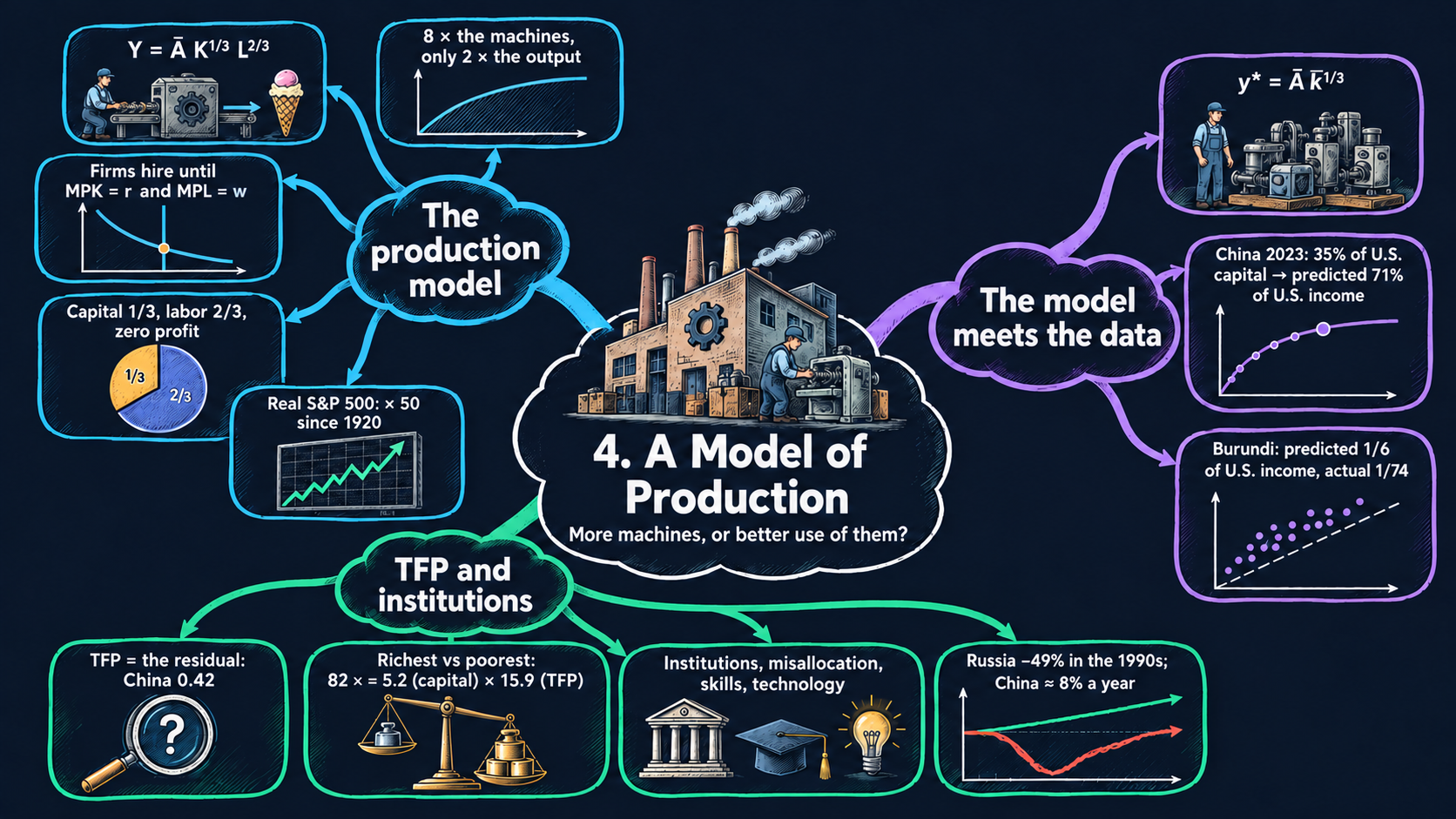
Come back to Islandia, the small imaginary island country of this book. Its people make one all-purpose good, counted in tons per year, with two inputs: workers and machines (its capital: boats, nets, workshops). Think of all of Islandia’s firms as one company, Harbor Boatworks, that rents every machine and hires every worker on the island. How much can Islandia make with what it has, and how is the output split between the workers and the owners of the machines? And if Islandia is poorer than another country, is that because it has fewer machines, or because it uses them less well? The production model answers both questions.

NoteThe big idea

The question. Why does a worker in a rich country produce many times more than a worker in a poor one?

The answer in one sentence. More machines per worker raise output, but with diminishing returns, so most of the gap between rich and poor countries comes from how well they combine their inputs: total factor productivity (TFP).

What goes in and what comes out. We choose productivity and the numbers of machines and workers. The model gives back output, the wage, the rental price of a machine, the income shares and output per person. Turned around, it measures TFP from data.

Road map.

1. The production model: the assumptions, solving the model from the firm’s choice to the market prices, and what the model predicts.
2. Development accounting: capital and TFP across countries: the assumptions, the steps that measure TFP and split an income gap, and what they show.
3. Model in code: the key results as Python functions, checked with numbers. Every later section reuses them.

Notation. A bar over a letter marks a parameter: a number we take as given from outside the model. Letters without a bar are endogenous variables: the model determines them. In the code we simply write A, K_bar and L_bar.

Symbol	Meaning	Type
\(Y, K, L\)	output (tons per year), machines and workers	endogenous
\(r, w\)	rental price of a machine and wage, both in tons of the good	endogenous
\(MPK, MPL\)	marginal products of capital and of labor	endogenous
\(\Pi\)	profit of the representative firm	endogenous
\(y, k\)	output and capital per person, \(Y/L\) and \(K/L\)	endogenous
\(\bar{A}\)	productivity; across countries we call it TFP	parameter
\(\bar{K}, \bar{L}\)	the machines and the workers Islandia has	parameters
\(\bar{k}\)	capital per person, \(\bar{K}/\bar{L}\)	parameter
\(\alpha\)	exponent on capital in the code (\(1/3\) in the text)	parameter
\(w^*, Y^*, \dots\)	an asterisk marks an equilibrium value	notation
\(\lambda\)	a factor that scales the inputs	notation

The production model

Assumptions

Five rules describe Islandia’s economy in any given year.

1. One good. Islandia does not trade with other countries and makes a single good, counted in tons per year. We quote every price in tons of this good, so the good’s own price is 1. A good that serves as the yardstick for all other prices is called the numéraire.

2. Fixed amounts of the inputs. Islandia has \(\bar{L}\) workers and \(\bar{K}\) machines. Both are parameters: this chapter takes them as given and does not ask where they came from. (The Solow model of Chapter 5 explains how the machines pile up.)

3. Technology. With \(K\) machines and \(L\) workers, Harbor Boatworks can make

\[Y = F(K, L) = \bar{A}K^{1/3}L^{2/3}, \tag{1}\]

the Cobb-Douglas production function. The inputs \(K\) and \(L\) have no bars here, on purpose: the function gives the output of any mix of inputs, not only of the mix Islandia owns. The positive number \(\bar{A}\) is productivity. With the same machines and the same workers, a higher \(\bar{A}\) means more tons.

4. Price-taking firms that maximize profit. Islandia has many identical firms. Each is too small to move the wage \(w\) or the rental price of capital \(r\), so it takes both prices as given. Each picks \(K\) and \(L\) to earn the largest profit it can. With constant returns to scale (shown next), the number of firms does not matter. So we treat them as one representative firm, Harbor Boatworks, that rents all the machines and hires all the workers.

5. Markets clear. The wage and the rental price move until Harbor Boatworks wants exactly the machines and the workers that Islandia has.

Equation (1) has two properties that drive the whole chapter. Both come from the rules for exponents, \((ab)^c = a^cb^c\) and \(a^ca^d = a^{c+d}\) (Appendix C.3).

Constant returns to scale. Scale both inputs by the same factor \(\lambda > 0\):

\[F(\lambda K, \lambda L) = \bar{A}(\lambda K)^{1/3}(\lambda L)^{2/3} = \lambda^{1/3}\lambda^{2/3}\,\bar{A}K^{1/3}L^{2/3} = \lambda^{1/3+2/3}F(K,L) = \lambda F(K,L).\]

The exponents add up to one, so output rises in exact proportion to the inputs. A sum above one would give increasing returns to scale, and a sum below one decreasing returns to scale. Constant returns is a natural benchmark because a firm can always copy itself: if Harbor Boatworks opens a twin of its yard, with the same crew and machines, the twin makes as many tons as the first.

Diminishing returns to one input. Now scale the machines alone:

\[F(\lambda K, L) = \bar{A}(\lambda K)^{1/3}L^{2/3} = \lambda^{1/3}F(K,L).\]

Twice the machines with the same crew give only \(2^{1/3} \approx 1.26\) times the output. Each new machine has fewer hands to run it, so it adds less than the one before. Take \(\bar{A} = 1\) and the 64 workers of Fig. 1. One machine gives \(1^{1/3}\times 64^{2/3} = 16\) tons, and eight machines give \(8^{1/3}\times 64^{2/3} = 2\times 16 = 32\) tons. That is eight times the machines, but only twice the output.

Doubling machines and workers together doubles output, but adding machines alone runs into diminishing returns.

NoteCheck your understanding

1. Harbor Boatworks has 64 workers, and \(\bar{A} = 1\). How many tons do 27 machines make? Compare the result with the 32 tons of 8 machines.

Answer

By equation (1), \(Y = 27^{1/3}\times 64^{2/3} = 3\times 16 = 48\) tons. The machines more than triple, from 8 to 27, but output grows only by the factor \(48/32 = 1.5\). That is diminishing returns to one input.

2. Islandia’s workforce and its stock of machines both double. What happens to output, and to output per worker?

Answer

Output doubles, by constant returns to scale: \(F(2K, 2L) = 2F(K, L)\). Output per worker, \(Y/L\), stays the same, because twice the tons are shared by twice the workers.

Solving the model

Step 1: the firm’s problem. Harbor Boatworks’ profit is what it sells minus what it pays for machines and workers. The good’s price is 1, so its sales are simply \(Y\):

\[\max_{K,L}\ \Pi = F(K,L) - rK - wL.\]

Step 2: the marginal products. The marginal product of capital, \(MPK\), is the extra output from one more machine, with the crew unchanged. The marginal product of labor, \(MPL\), is the extra output from one more worker, with the machines unchanged. For small changes, these are the partial derivatives of \(F\) (Appendix C.7). Hold \(L\) constant and apply the power rule, \(\frac{d}{dK}K^{a} = aK^{a-1}\):

\[MPK = \frac{\partial F}{\partial K} = \frac{1}{3}\bar{A}K^{1/3-1}L^{2/3} = \frac{1}{3}\bar{A}K^{-2/3}L^{2/3}.\]

Two rewritings make this easier to read. First, \(K^{-2/3}L^{2/3} = (L/K)^{2/3}\). Second, \(K^{-2/3} = K^{1/3}/K\), so \(\bar{A}K^{-2/3}L^{2/3} = \bar{A}K^{1/3}L^{2/3}/K = Y/K\). Together they give

\[MPK = \frac{1}{3}\bar{A}\left(\frac{L}{K}\right)^{2/3} = \frac{1}{3}\cdot\frac{Y}{K}.\]

Now hold \(K\) constant instead and use \(L^{2/3-1} = L^{-1/3}\):

\[MPL = \frac{\partial F}{\partial L} = \frac{2}{3}\bar{A}K^{1/3}L^{-1/3} = \frac{2}{3}\bar{A}\left(\frac{K}{L}\right)^{1/3} = \frac{2}{3}\cdot\frac{Y}{L}.\]

ImportantKey result: the marginal products

\[MPK = \frac{1}{3}\bar{A}\left(\frac{L}{K}\right)^{2/3} = \frac{1}{3}\cdot\frac{Y}{K} \tag{2}\]

\[MPL = \frac{2}{3}\bar{A}\left(\frac{K}{L}\right)^{1/3} = \frac{2}{3}\cdot\frac{Y}{L} \tag{3}\]

With a Cobb-Douglas function, each marginal product is the input’s exponent times its average product: tons per machine, \(Y/K\), or tons per worker, \(Y/L\).

TipIn words

The middle form of equation (2) shows diminishing returns at work. If Harbor Boatworks adds machines but keeps its crew, \(L/K\) falls, and so does the MPK. If it hires more workers instead, the MPK rises: every machine now has more hands to run it. Equation (3) tells the same story with the two inputs swapped.

Step 3: the hiring rules. At the best choice of inputs, the derivative of profit with respect to each input is zero (Appendix C.8):

\[\frac{\partial \Pi}{\partial K} = MPK - r = 0, \qquad \frac{\partial \Pi}{\partial L} = MPL - w = 0.\]

The same rule follows without calculus. If one more machine adds more tons than its rent, \(MPK > r\), renting it raises profit, so Harbor Boatworks rents more and the MPK falls. If \(MPK < r\), handing a machine back raises profit. Only at \(MPK = r\) is nothing left to gain. In the same way, the firm hires workers until \(MPL = w\). The MPK falls as \(K\) rises, so the rule \(r = \frac{1}{3}\bar{A}(L/K)^{2/3}\) is a downward-sloping demand curve for capital, with capital \(K\) on the x-axis and its rental price \(r\) on the y-axis. Likewise, the MPL curve is the demand curve for labor.

Step 4: five equations in five unknowns. The model has to find three quantities, \(Y\), \(K\) and \(L\), and two prices, \(r\) and \(w\):

Equation	Role
\(Y = \bar{A}K^{1/3}L^{2/3}\)	production function
\(r = \frac{1}{3}\cdot\frac{Y}{K}\)	hiring rule for capital: demand for capital
\(w = \frac{2}{3}\cdot\frac{Y}{L}\)	hiring rule for labor: demand for labor
\(K = \bar{K}\)	the capital market clears
\(L = \bar{L}\)	the labor market clears

The parameters are \(\bar{A}\), \(\bar{K}\) and \(\bar{L}\). Both input markets clear at the same time, so the solution is a general equilibrium, not the partial equilibrium of one market on its own.

Step 5: solve. The two market-clearing conditions give the quantities at once: \(K^* = \bar{K}\) and \(L^* = \bar{L}\). The supply curves are vertical lines at \(\bar{K}\) and \(\bar{L}\), so every machine and every islander is at work. Putting them into the production function gives output, \(Y^* = \bar{A}\bar{K}^{1/3}\bar{L}^{2/3}\). Putting \(Y^*\) into the hiring rules gives the prices. For the rental price, divide by \(\bar{K}\) and subtract exponents, \(\bar{K}^{1/3}/\bar{K} = \bar{K}^{-2/3}\):

\[r^* = \frac{1}{3}\cdot\frac{\bar{A}\bar{K}^{1/3}\bar{L}^{2/3}}{\bar{K}} = \frac{1}{3}\bar{A}\bar{K}^{-2/3}\bar{L}^{2/3} = \frac{1}{3}\bar{A}\left(\frac{\bar{L}}{\bar{K}}\right)^{2/3}.\]

For the wage, divide by \(\bar{L}\) and use \(\bar{L}^{2/3}/\bar{L} = \bar{L}^{-1/3}\):

\[w^* = \frac{2}{3}\cdot\frac{\bar{A}\bar{K}^{1/3}\bar{L}^{2/3}}{\bar{L}} = \frac{2}{3}\bar{A}\bar{K}^{1/3}\bar{L}^{-1/3} = \frac{2}{3}\bar{A}\left(\frac{\bar{K}}{\bar{L}}\right)^{1/3}.\]

We now collect the results, with each unknown on the left and only parameters on the right.

ImportantKey result: the equilibrium of the production model

\[\begin{aligned} K^* &= \bar{K}, \qquad L^* = \bar{L}, \qquad Y^* = \bar{A}\bar{K}^{1/3}\bar{L}^{2/3},\\ r^* &= \frac{1}{3}\bar{A}\left(\frac{\bar{L}}{\bar{K}}\right)^{2/3}, \qquad w^* = \frac{2}{3}\bar{A}\left(\frac{\bar{K}}{\bar{L}}\right)^{1/3}. \end{aligned} \tag{4}\]

Islandia in numbers. With the values of Fig. 2, \(\bar{K} = \bar{L} = \bar{A} = 1\), Islandia makes \(Y^* = 1\) ton, a machine rents for \(r^* = 1/3\) of a ton and a worker earns \(w^* = 2/3\) of a ton.

TipIn words: what Islandia makes and what it pays

No machine and no islander sits idle, so Islandia makes all it can. Each input is paid what its last unit adds: machines rent cheaply when they are plentiful, and workers earn more when each has many machines.

Step 6: who gets what. Multiply the wage by employment and divide by output. The hiring rule says \(w^* = \frac{2}{3}Y^*/L^*\), so \(L^*\) and \(Y^*\) cancel:

\[\frac{w^*L^*}{Y^*} = \frac{2}{3}\cdot\frac{Y^*}{L^*}\cdot\frac{L^*}{Y^*} = \frac{2}{3}, \qquad\text{and in the same way}\qquad \frac{r^*K^*}{Y^*} = \frac{1}{3}\cdot\frac{Y^*}{K^*}\cdot\frac{K^*}{Y^*} = \frac{1}{3}. \tag{5}\]

These are the factor shares of income. They equal the exponents of the production function, whatever the values of \(\bar{A}\), \(\bar{K}\) and \(\bar{L}\). This is why we put the exponent \(1/3\) on capital: in U.S. data, capital earns roughly a third of GDP and labor roughly two-thirds, and the split has moved little over time (Chapter 2). The two shares add up to one, \(2/3 + 1/3 = 1\). Multiply through by \(Y^*\):

\[w^*L^* + r^*K^* = Y^*. \tag{6}\]

Wages and rents together use up every ton Islandia makes, so economic profit is zero, \(\Pi^* = Y^* - r^*K^* - w^*L^* = 0\), as perfect competition leads us to expect. Equation (6) also says that total income equals total production, an identity of national income accounting; since all output is consumed, it equals spending too. What accountants call profit is the payment to capital, \(r^*K^* = Y^*/3\), and the stock market puts a price on claims to this flow of capital income (Fig. 3).

Step 7: per person. Living standards depend on output per person, \(y \equiv Y/L\). Let \(k \equiv K/L\) be capital per person. (Every islander works in this model, so “per person” and “per worker” mean the same thing.) Divide \(Y^*\) by \(\bar{L}\) and use \(\bar{L}^{2/3}/\bar{L} = \bar{L}^{-1/3}\):

\[y^* = \frac{Y^*}{L^*} = \frac{\bar{A}\bar{K}^{1/3}\bar{L}^{2/3}}{\bar{L}} = \bar{A}\bar{K}^{1/3}\bar{L}^{-1/3} = \bar{A}\left(\frac{\bar{K}}{\bar{L}}\right)^{1/3}.\]

Write \(\bar{k} = \bar{K}/\bar{L}\) for the machines per worker, and the result takes its shortest form.

ImportantKey result: output per person

\[y^* = \bar{A}\bar{k}^{1/3} \tag{7}\]

The prices can be written per person too: \(w^* = \frac{2}{3}y^*\), so the wage moves in step with income per person, and \(r^* = \frac{1}{3}y^*/\bar{k} = \frac{1}{3}\bar{A}\bar{k}^{-2/3}\).

Islandia in numbers. With the 8 machines and 64 workers of Fig. 1 and \(\bar{A} = 1\), \(\bar{k} = 1/8\). So \(y^* = (1/8)^{1/3} = 1/2\) ton per worker, and the wage is \(w^* = \frac{2}{3}\cdot\frac{1}{2} = 1/3\) of a ton.

TipIn words

An islander’s income rests on two things: how productive Islandia is, and how many machines each worker has. Productivity raises income one for one. More machines per worker raise it too, but the cube root means that each extra machine per worker adds less than the one before.

A general exponent. The code lets the exponent on capital be any \(\alpha\) between 0 and 1, so that \(Y = \bar{A}K^{\alpha}L^{1-\alpha}\). The same steps give \(MPK = \alpha Y/K\), \(MPL = (1-\alpha)Y/L\), factor shares \(\alpha\) and \(1-\alpha\), and \(y^* = \bar{A}\bar{k}^{\alpha}\). Setting \(\alpha = 1/3\) brings back equations (2) to (7).

Each input earns its marginal product, and these payments use up exactly all of Islandia’s output: one-third to machines, two-thirds to workers.

NoteCheck your understanding

1. Harbor Boatworks runs 8 machines with 64 workers, and \(\bar{A} = 1\), so it makes 32 tons. What are the rental price and the wage? How many tons go to the workers, and how many to the owners of the machines?

Answer

By equation (2), \(r^* = \frac{1}{3}\cdot\frac{32}{8} = 4/3\) of a ton per machine. By equation (3), \(w^* = \frac{2}{3}\cdot\frac{32}{64} = 1/3\) of a ton per worker. Workers get \(64\times\frac{1}{3} \approx 21.3\) tons and machine owners get \(8\times\frac{4}{3} \approx 10.7\) tons: two-thirds and one-third of output (equation 5), adding up to all 32 tons (equation 6).

2. Suppose Harbor Boatworks paid a wage below the marginal product of labor. What would it want to do, and why can that not last?

Answer

Each extra worker would add more tons than the wage costs, so profit would rise with every hire, and the firm would want more workers than Islandia has. All islanders already work (\(L = \bar{L}\)), so firms compete for them and bid the wage up until \(w = MPL\), the hiring rule of step 3.

What the model predicts

Comparative statics. What happens to the equilibrium when a parameter changes? Take logs of the solution (4) and of equation (7) (Appendix C.4). The log of a product is the sum of the logs, and the log of a power is the exponent times the log:

\[\ln Y^* = \ln\bar{A} + \tfrac{1}{3}\ln\bar{K} + \tfrac{2}{3}\ln\bar{L}, \qquad \ln y^* = \ln\bar{A} + \tfrac{1}{3}\ln\bar{K} - \tfrac{1}{3}\ln\bar{L},\]

\[\ln w^* = \ln\tfrac{2}{3} + \ln\bar{A} + \tfrac{1}{3}\ln\bar{K} - \tfrac{1}{3}\ln\bar{L}, \qquad \ln r^* = \ln\tfrac{1}{3} + \ln\bar{A} - \tfrac{2}{3}\ln\bar{K} + \tfrac{2}{3}\ln\bar{L}.\]

Each coefficient is an elasticity: the percent change in the variable when the parameter rises by 1 percent.

A 1% rise in …	\(Y^*\)	\(y^*\)	\(w^*\)	\(r^*\)	What moves in Fig. 2
productivity \(\bar{A}\)	\(+1\%\)	\(+1\%\)	\(+1\%\)	\(+1\%\)	both demand curves (MPK and MPL) shift up
capital \(\bar{K}\)	\(+\tfrac{1}{3}\%\)	\(+\tfrac{1}{3}\%\)	\(+\tfrac{1}{3}\%\)	\(-\tfrac{2}{3}\%\)	the capital supply line shifts right; labor demand shifts up
labor \(\bar{L}\)	\(+\tfrac{2}{3}\%\)	\(-\tfrac{1}{3}\%\)	\(-\tfrac{1}{3}\%\)	\(+\tfrac{2}{3}\%\)	the labor supply line shifts right; capital demand shifts up
both \(\bar{K}\) and \(\bar{L}\)	\(+1\%\)	\(0\)	\(0\)	\(0\)	both supply lines shift right

The factor shares of equation (5) stay at \(1/3\) and \(2/3\) in every row. For \(y^* = Y^*/\bar{L}\), the elasticity with respect to \(\bar{L}\) is \(2/3 - 1 = -1/3\), because the same output is now shared by more people.

What the table tells us about Islandia:

• Each input is worth more when the other one is plentiful. More machines lower their own rental price, a move down the capital demand curve, because of diminishing returns. But they raise the wage, since every worker now has more machines to use. More workers do the opposite.
• Prices depend only on the ratio \(\bar{K}/\bar{L}\). Scaling up the whole economy raises total output but changes nothing per person. A country is not richer per person just because it is bigger.
• Productivity is the one parameter that raises every outcome, each with an elasticity of 1.
• Capital per person has diminishing returns. By equation (7), doubling \(\bar{k}\) multiplies \(y^*\) by \(2^{1/3} \approx 1.26\). Large gaps in capital per person therefore turn into much smaller gaps in income. The second block takes this prediction to the data.

With the values of Fig. 2, doubling \(\bar{K}\) from 1 to 2 lowers the rental price from \(1/3 \approx 0.333\) to \(\frac{1}{3}(1/2)^{2/3} \approx 0.210\) and raises the wage from \(2/3 \approx 0.667\) to \(\frac{2}{3}\cdot 2^{1/3} \approx 0.840\).

More machines lower their own rent but raise wages, and productivity is the only parameter that lifts every outcome.

NoteCheck your understanding

1. Islandia’s workforce grows by 10 percent, with the same machines and the same productivity. By roughly what percentage do the wage and the rental price change? Then compute the exact changes.

Answer

The elasticities with respect to \(\bar{L}\) are \(-1/3\) for \(w^*\) and \(+2/3\) for \(r^*\), so the wage falls by roughly 3.3 percent and the rental price rises by roughly 6.7 percent. Exactly, by equation (4), the wage is multiplied by \(1.1^{-1/3} \approx 0.969\), a fall of about 3.1 percent, and the rental price by \(1.1^{2/3} \approx 1.066\), a rise of about 6.6 percent. Each machine now has more hands, and each worker fewer machines.

2. Better know-how raises Islandia’s \(\bar{A}\) by 10 percent. Does the workers’ share of income rise?

Answer

No. The wage rises by 10 percent (elasticity 1), but so does output, so the labor share stays at \(w^*L^*/Y^* = 2/3\) (equation 5). Only the exponent of the production function can change the shares.

Development accounting: capital and TFP across countries

Assumptions

We now use equation (7) to compare whole countries. In the data, the benchmark is the United States. In our story, we compare Islandia with Mainland, which plays the role of the rich benchmark. This exercise is called development accounting, and it adds three assumptions:

• every country produces with the same Cobb-Douglas function, with the exponent \(1/3\) on capital that matches capital’s share of income in the data;
• \(y\) is measured as real GDP per person, and \(\bar{k}\) as the stock of physical capital (buildings, machinery, equipment, computers) per person;
• both are measured relative to the benchmark (the United States in the data, Mainland in the story), so the benchmark’s values are 1.

As a first pass, we also assume that productivity is the same everywhere, \(\bar{A} = 1\).

Solving the model

Step 1: compare two countries. Write equation (7) for a country \(i\) (Islandia, say) and for the benchmark, labeled \(US\) as in the data, and divide. A ratio of two powers with the same exponent is the power of the ratio, \(a^c/b^c = (a/b)^c\):

\[\frac{y^*_i}{y^*_{US}} = \frac{\bar{A}_i}{\bar{A}_{US}}\left(\frac{\bar{k}_i}{\bar{k}_{US}}\right)^{1/3}.\]

Step 2: equal productivity. If \(\bar{A}_i = \bar{A}_{US}\), and \(y\) and \(\bar{k}\) are both measured relative to the benchmark, the prediction is simply

\[y^* = \bar{k}^{1/3}.\]

In logs, \(\ln y^* = \frac{1}{3}\ln\bar{k}\): a gap in capital per person becomes an income gap only one-third as large in logs. Suppose Islandia has one-eighth of Mainland’s capital per person. The model then predicts that Islandia has \((1/8)^{1/3} = 1/2\) of Mainland’s income. With \(1/27\) of the capital, the prediction would be \(1/3\) of the income.

TipIn words: diminishing returns squeeze the gaps

Each extra machine per worker adds less than the one before, so a country with far fewer machines is only somewhat poorer. If capital were the only difference, poor countries would be much richer than they are (Figs. 4 and 5).

Step 3: measure TFP. We have data on \(y\) and \(\bar{k}\) for every country, but no direct way to measure \(\bar{A}\). So we assume the model is right, and solve equation (7) for the one term we cannot see. Dividing both sides of \(y^* = \bar{A}\bar{k}^{1/3}\) by \(\bar{k}^{1/3}\):

ImportantKey result: total factor productivity

\[\bar{A} = \frac{y^*}{\bar{k}^{1/3}} \tag{8}\]

This \(\bar{A}\) is total factor productivity (TFP): the output a country gets from given amounts of capital and labor.

Islandia in numbers. Suppose Islandia has one-eighth of Mainland’s capital per person and also one-eighth of its income. Its predicted income with Mainland’s TFP is \(1/2\), so its implied TFP is \((1/8)/(1/2) = 1/4\).

TFP is chosen so that the model fits exactly. That makes it a residual: it collects everything other than physical capital that raises income, and so it measures how much the model leaves unexplained.

Step 4: split an income gap. Write equation (7) for a rich country and a poor one, and divide them. The result splits the income gap into two factors.

ImportantKey result: splitting an income gap

\[\frac{y^*_{rich}}{y^*_{poor}} = \frac{\bar{A}_{rich}}{\bar{A}_{poor}}\times\left(\frac{\bar{k}_{rich}}{\bar{k}_{poor}}\right)^{1/3} \tag{9}\]

The first factor is the TFP part of the gap, and the second is the capital part.

Islandia in numbers. Mainland is 8 times richer than Islandia: \(8 = 4\times 2\), a factor of 4 from TFP and a factor of 2 from capital.

Taking logs turns the product into a sum, so the two parts of the log gap add up exactly:

\[\underbrace{\ln\frac{y^*_{rich}}{y^*_{poor}}}_{\text{income gap}} = \underbrace{\ln\frac{\bar{A}_{rich}}{\bar{A}_{poor}}}_{\text{TFP part}} + \underbrace{\tfrac{1}{3}\ln\frac{\bar{k}_{rich}}{\bar{k}_{poor}}}_{\text{capital part}}.\]

For Islandia and Mainland, capital explains \(\ln 2/\ln 8 = 1/3\) of the log gap, and TFP explains \(\ln 4/\ln 8 = 2/3\).

Step 5: the return to capital across countries. Per person, equation (2) reads \(MPK = \frac{1}{3}y/\bar{k} = \frac{1}{3}\bar{A}\bar{k}^{-2/3}\). Dividing for two countries,

\[\frac{MPK_{poor}}{MPK_{rich}} = \frac{\bar{A}_{poor}}{\bar{A}_{rich}}\left(\frac{\bar{k}_{rich}}{\bar{k}_{poor}}\right)^{2/3}.\]

With equal TFP, Islandia, with one-eighth of the capital, would have a marginal product \(8^{2/3} = 4\) times Mainland’s, and Mainland’s investors would rush to move machines to the island. With a TFP of \(1/4\), the two effects cancel exactly, \(\frac{1}{4}\times 4 = 1\), and a machine earns the same return in both places. Low TFP thus answers a question Robert Lucas asked in 1990: why does so little capital flow from rich to poor countries?

A capital gap shrinks to its cube root in income, so TFP has to carry most of the income gap.

NoteCheck your understanding

1. Suppose instead that Islandia has \(1/27\) of Mainland’s capital per person and \(1/9\) of its income. What income does the model predict with equal TFP? What is Islandia’s implied TFP, and what share of the log income gap does capital explain?

Answer

With equal TFP, \(y^* = (1/27)^{1/3} = 1/3\). By equation (8), TFP is \((1/9)/(1/3) = 1/3\). By equation (9), the gap of 9 splits into \(3\times 3\): a factor of 3 from TFP and 3 from capital. In logs, capital explains \(\ln 3/\ln 9 = 1/2\) of the gap.

What the model predicts

Result	Elasticity	In words
income, \(y^* = \bar{A}\bar{k}^{1/3}\)	\(1/3\) for \(\bar{k}\), \(1\) for \(\bar{A}\)	capital gaps are compressed; TFP gaps pass through in full
implied TFP, \(\bar{A} = y^*/\bar{k}^{1/3}\)	\(1\) for \(y^*\), \(-1/3\) for \(\bar{k}\)	a country poorer than its capital predicts has low TFP
return to capital, \(MPK = \frac{1}{3}\bar{A}\bar{k}^{-2/3}\)	\(-2/3\) for \(\bar{k}\), \(1\) for \(\bar{A}\)	capital-poor countries earn high returns only if their TFP is not too low

• With equal productivity, the model fails in a telling way. It ranks countries correctly, but its income gaps are far too small: nearly every country is poorer than its capital predicts.
• A bigger exponent is no fix. With \(y^* = \bar{k}^{\alpha}\) and \(\alpha = 1\), income gaps would be as large as capital gaps. Then most poor countries fall below the 45-degree line, while most rich ones stay slightly above it. It also clashes with a capital share of about one-third (try it with the slider of Fig. 5).
• TFP explains most of the gap. When rich and poor countries are compared, TFP typically accounts for about two-thirds or more of the log income gap, and capital for the rest (Figs. 6 and 7 and the key numbers after them).
• What is TFP? The model takes \(\bar{A}\) as a parameter and does not explain it. The usual suspects are:
  • human capital (skills and schooling);
  • technology;
  • institutions (secure property rights, courts that enforce contracts, and the rule of law);
  • misallocation: capital and labor placed in the wrong firms.
  We can size the role of human capital with \(w^* = \frac{2}{3}y^*\): if extra schooling raises wages by some percentage, it raises income per person by the same percentage. In the data this explains part of the measured TFP gap, but far from all of it.

Most of the income gap between rich and poor countries comes from TFP, which this model measures but does not explain.

NoteCheck your understanding

1. Suppose Islandia’s statistics overstate its stock of machines. Is its measured TFP too high or too low?

Answer

Too low. Equation (8) divides income by \(\bar{k}^{1/3}\), so a capital number that is too large gives an \(\bar{A}\) that is too small. TFP is a residual, so every error in measuring capital ends up in it.

2. In the example of the previous check (\(1/27\) of Mainland’s capital, TFP of \(1/3\)), would Mainland’s investors want to move machines to Islandia?

Answer

Yes. By the formula of step 5, \(MPK_{Islandia}/MPK_{Mainland} = \frac{1}{3}\times 27^{2/3} = \frac{1}{3}\times 9 = 3\). Low TFP cuts the return on Islandia, but not by enough: a machine there still earns three times as much.

NoteRecap

• Production with diminishing returns: \(Y = \bar{A}K^{1/3}L^{2/3}\) has constant returns to scale, but each extra machine adds less output than the one before (Fig. 1).
• Prices equal marginal products: the MPK and MPL curves are the demand curves, and the fixed supplies of machines and workers set \(r^*\) and \(w^*\) (Fig. 2).
• One-third to capital, two-thirds to labor: the payments use up all of output, profit is zero, and the stock market prices the income of capital (Fig. 3).
• Capital alone predicts too little inequality: with equal TFP, \(y^* = \bar{k}^{1/3}\), and nearly every country is poorer than its capital predicts (Fig. 5).
• TFP is the residual that closes the gap: \(\bar{A} = y^*/\bar{k}^{1/3}\), and it explains most of the income difference between rich and poor countries (Fig. 7).

Model in code

Now we turn the Key results into Python. The section has three parts: the setup (folded, because it is the same in every chapter), the model as functions, and numerical checks of the Key results. Run its cells once, in order. Every later section of the notebook reuses them.

Setup

Run the setup cells once, before anything else. They load the Python libraries, give every chart the same look, store the address of the chapter’s data and define two helpers that only the book website needs. You can use the notebook without reading them; open the box if you are curious.

NoteShow the setup code

The first cell loads the libraries and sets the look of the charts. Its comments explain each step.

# @title Setup: libraries, chart colors and the data location
# Text after a "#" is a comment: Python ignores it, it is there for human readers.

# Step 1: load the libraries. `import` loads a library, a toolbox written by
# other people, and `as np` gives it a short nickname, so the code stays short.
import numpy as np                              # numbers and arrays
import pandas as pd                             # data tables
import plotly.express as px                     # quick charts from data tables
# charts built piece by piece (the model figures)
import plotly.graph_objects as go
import plotly.io as pio                         # settings shared by every chart
from plotly.subplots import make_subplots       # several panels in one figure
# sliders, buttons and menus for the interactive figures
from ipywidgets import (interact, fixed, FloatSlider, SelectionSlider, IntRangeSlider, ToggleButtons,
                        Dropdown, SelectMultiple)

# Step 2: one light blue/green look for every chart
BLUE, TEAL, GREEN, GRAY = "#16528c", "#008070", "#7fb23a", "#8a96a3"
pio.templates.default = "plotly_white"
# the same chart size in Colab and on the website
pio.templates["plotly_white"].layout.update(width=860, height=480)
px.defaults.color_discrete_sequence = [BLUE, TEAL, GREEN, "#5aa0d8", "#0b4f47"]
WIDE = {"description_width": "initial"}         # show the full slider labels

# Step 3, Colab only: let Plotly charts appear inside the interactive widgets.
# `try` runs the indented lines; if the import fails (we are not in Colab),
# `except` skips them.
try:
    import google.colab
    google.colab.output.enable_custom_widget_manager()
except ImportError:
    pass                                        # not running in Colab: nothing to do

# Step 4: the data files of this chapter live in the book's GitHub repository
DATA_URL = "https://raw.githubusercontent.com/quarcs-lab/macro102-site/main/data/ch04/"

The website cannot run Python, so each interactive figure also gets a version with a precomputed slider. The next two helpers build those versions. Run them and move on.

# @title Helper for the website versions (run this cell; you do not need to read it)
def slider_figure(make_figure, name, values, start, label=None):
    """Join precomputed versions of a figure with one slider (the website cannot run Python).

    Arguments
        make_figure : the function that draws the figure, e.g. production_curve
        name        : the argument the slider moves, e.g. "L"
        values      : the values of that argument to precompute
        start       : the value shown first
        label       : the slider's label (the argument name if None)
    Returns
        one Plotly figure with all versions and a slider that shows one at a time
    """
    # Step 1: draw the figure once for every value
    figures = [make_figure(**{name: v}) for v in values]
    first = values.index(start)
    # Step 2: copy every curve into one figure; only the start value's are visible
    fig = go.Figure(layout=figures[first].layout)
    owner = []                          # which precomputed figure each trace is from
    for i, f in enumerate(figures):
        for trace in f.data:
            trace.visible = (i == first)
            fig.add_trace(trace)
            owner.append(i)
    # Step 3: one slider step per value: its curves, title, labels and shapes
    steps = []
    for i, f in enumerate(figures):
        layout = {"title": f.layout.title.to_plotly_json(),
                  "annotations": [a.to_plotly_json() for a in f.layout.annotations],
                  "shapes": [s.to_plotly_json() for s in f.layout.shapes]}
        visible = [o == i for o in owner]
        steps.append(dict(method="update", label=str(values[i]), args=[{"visible": visible}, layout]))
    fig.update_layout(sliders=[dict(active=first, steps=steps, pad=dict(t=60),
                                    currentvalue=dict(prefix=(label or name) + " = "))])
    return fig

# @title Helper for the website versions with many countries (run this cell; you do not need to read it)
def country_menu(fig, shown, regions, label="Textbook countries"):
    """Draw the countries in `shown` and put every other country one click away in the legend.

    With more than 40 countries, a menu above the plot chooses the region whose countries the legend lists.
    Traces that are not countries stay as they are.

    Arguments
        fig     : a Plotly figure with one trace per country
        shown   : the countries drawn at the start
        regions : maps each country to its region
        label   : the name of the first menu entry
    Returns
        the same figure, with the visibility set and, for many countries, the region menu
    """
    # Step 1: the menu entries, the textbook countries and then one entry per region
    # the traces that are countries, and each of their regions once, A to Z
    countries = [trace.name for trace in fig.data if trace.name in regions]
    groups = [label] + sorted(set(regions[name] for name in countries))
    if len(countries) <= 40:
        groups = [None]                     # a short legend lists every country at once
    # Step 2: for each entry, which traces are drawn, in the legend only, or hidden
    buttons = []
    for group in groups:
        visible = []
        for trace in fig.data:
            if trace.name in shown:
                visible.append(True)                    # a textbook country: drawn
            elif trace.name not in regions:
                # not a country: as it was
                visible.append(True if trace.visible is None else trace.visible)
            elif group is None or regions[trace.name] == group:
                visible.append("legendonly")            # in this region: a click away
            else:
                visible.append(False)                   # another region: hidden
        buttons.append(dict(label=group, method="restyle", args=[{"visible": visible}]))
    # Step 3: start with the first entry, and add the menu when there is more than one
    for trace, v in zip(fig.data, buttons[0]["args"][0]["visible"]):
        trace.visible = v
    if len(groups) > 1:
        menu = dict(type="dropdown", buttons=buttons, x=1, xanchor="right", y=1.02, yanchor="bottom")
        fig.update_layout(updatemenus=list(fig.layout.updatemenus) + [menu], margin=dict(t=110))
    return fig

The model as functions

Three Key results hold the whole model: the production function, equation (1), and the marginal products, equations (2) and (3), which are also the equilibrium prices. We write each one as a Python function: a named recipe that takes inputs and gives back a result. To let you experiment with the shape of the function, the code writes the exponent on capital as \(\alpha\) (“alpha”), with the textbook value \(\alpha = 1/3\) as the default.

# `def` creates a function. Its inputs are the arguments in parentheses.
# `A=1.0` gives A a default value, used whenever we do not pass one.
# The text in triple quotes describes the function.
def production(K, L, A=1.0, alpha=1 / 3):
    """Output, from the Cobb-Douglas production function.

    Equation (1):  Y = A K^alpha L^(1 - alpha), with alpha = 1/3 in the textbook

    Arguments
        K     : capital, the number of machines
        L     : labor, the number of workers
        A     : productivity, A-bar (1 unless we pass another value)
        alpha : the exponent on capital (1/3 unless we pass another value)
    Returns
        output, Y
    """
    # `return` gives back the result; `**` means "to the power of",
    # and `1 / 3` is simply the number one third
    return A * K ** alpha * L ** (1 - alpha)

The marginal products are the extra output from one more machine and from one more worker. In equilibrium they are the rental price of capital and the wage. Both are a share of output per unit of the input.

def mpk(K, L, A=1.0, alpha=1 / 3):
    """Marginal product of capital, MPK.

    Equation (2):  MPK = alpha Y / K

    Arguments
        K, L  : capital and labor
        A     : productivity, A-bar
        alpha : the exponent on capital
    Returns
        the marginal product of capital, which is r* in equilibrium
    """
    # one-third of output per machine
    return alpha * production(K, L, A, alpha) / K


def mpl(K, L, A=1.0, alpha=1 / 3):
    """Marginal product of labor, MPL.

    Equation (3):  MPL = (1 - alpha) Y / L

    Arguments
        K, L  : capital and labor
        A     : productivity, A-bar
        alpha : the exponent on capital
    Returns
        the marginal product of labor, which is w* in equilibrium
    """
    # two-thirds of output per worker
    return (1 - alpha) * production(K, L, A, alpha) / L

Checking the key results

The formulas came from algebra. Now we check them with numbers, one Key result at a time.

Check 1: the production function. With \(\bar{A} = 1\) and 64 workers, Harbor Boatworks should make 32 tons with 8 machines. Doubling both inputs should double output, and doubling capital alone should multiply it by only \(2^{1/3}\).

# Harbor Boatworks with 8 machines and 64 workers, then with more inputs.
# An f-string, f"... {value:.2f}", puts a value into the text;
# ":.2f" means "two decimals".
print(f"8 machines and 64 workers:       Y = {production(8, 64):.2f} tons")
# constant returns to scale: double both inputs, double the output
print(f"Double both (16 and 128):        Y = {production(16, 128):.2f} tons   (constant returns: twice as much)")
# diminishing returns: double capital alone, output grows by only 2^(1/3)
print(f"Double capital only (16 and 64): Y = {production(16, 64):.2f} tons   (2^(1/3) = {2 ** (1 / 3):.3f} times as much)")
# the 2nd machine adds more than the 8th
print(f"Gain from the 2nd machine: {production(2, 64) - production(1, 64):.2f} tons; "
      f"from the 8th: {production(8, 64) - production(7, 64):.2f} tons")

8 machines and 64 workers:       Y = 32.00 tons
Double both (16 and 128):        Y = 64.00 tons   (constant returns: twice as much)
Double capital only (16 and 64): Y = 40.32 tons   (2^(1/3) = 1.260 times as much)
Gain from the 2nd machine: 4.16 tons; from the 8th: 1.39 tons

Check 2: the marginal products. Equations (2) and (3) came from derivatives. A derivative is the extra output from a very small extra amount of an input, divided by that amount, so we can compute it a second way with a tiny step.

# Step 1: 8 machines, 64 workers, and a tiny step for the derivative
K, L, small = 8, 64, 0.0001
# Step 2: MPK in two forms of equation (2), then as (extra output) / (small step)
print(f"MPK, equation (2), (1/3) Y/K:          {mpk(K, L):.4f}")
print(f"MPK, equation (2), (1/3) A (L/K)^(2/3): {(1 / 3) * (L / K) ** (2 / 3):.4f}")
print(f"MPK by a small step in K:              {(production(K + small, L) - production(K, L)) / small:.4f}")
# Step 3: the same three ways for MPL, equation (3)
print(f"MPL, equation (3), (2/3) Y/L:          {mpl(K, L):.4f}")
print(f"MPL, equation (3), (2/3) A (K/L)^(1/3): {(2 / 3) * (K / L) ** (1 / 3):.4f}")
print(f"MPL by a small step in L:              {(production(K, L + small) - production(K, L)) / small:.4f}")

MPK, equation (2), (1/3) Y/K:          1.3333
MPK, equation (2), (1/3) A (L/K)^(2/3): 1.3333
MPK by a small step in K:              1.3333
MPL, equation (3), (2/3) Y/L:          0.3333
MPL, equation (3), (2/3) A (K/L)^(1/3): 0.3333
MPL by a small step in L:              0.3333

Check 3: the equilibrium, the factor shares and zero profit. For three different economies, we compute the prices as marginal products and compare them with the closed forms of equation (4). Whatever the economy, capital should get one-third of output, labor two-thirds (equation 5), and nothing should be left as profit (equation 6).

# The `for` loop runs its indented lines once for each item of the list. Each item is
# a tuple, three numbers in parentheses, and `for K_bar, L_bar, A in` names them.
for K_bar, L_bar, A in [(1, 1, 1), (2, 1, 1), (8, 64, 1.5)]:
    # Step 1: output and the prices r* = MPK and w* = MPL
    Y_star = production(K_bar, L_bar, A)
    r_star, w_star = mpk(K_bar, L_bar, A), mpl(K_bar, L_bar, A)
    # Step 2: the same prices from the closed forms, and the profit left over
    r_formula = (1 / 3) * A * (L_bar / K_bar) ** (2 / 3)        # equation (4)
    w_formula = (2 / 3) * A * (K_bar / L_bar) ** (1 / 3)        # equation (4)
    profit = Y_star - r_star * K_bar - w_star * L_bar           # equation (6) says zero
    # Step 3: print the prices, the shares (equation 5) and the profit. `abs` is the
    # absolute value: it avoids printing a tiny rounding error as -0.000.
    print(f"K = {K_bar}, L = {L_bar}, A = {A}:  r* = {r_star:.3f} (formula {r_formula:.3f}),  "
          f"w* = {w_star:.3f} (formula {w_formula:.3f})")
    print(f"     capital share {r_star * K_bar / Y_star:.3f},  labor share {w_star * L_bar / Y_star:.3f},  "
          f"profit {abs(profit):.3f}")

K = 1, L = 1, A = 1:  r* = 0.333 (formula 0.333),  w* = 0.667 (formula 0.667)
     capital share 0.333,  labor share 0.667,  profit 0.000
K = 2, L = 1, A = 1:  r* = 0.210 (formula 0.210),  w* = 0.840 (formula 0.840)
     capital share 0.333,  labor share 0.667,  profit 0.000
K = 8, L = 64, A = 1.5:  r* = 2.000 (formula 2.000),  w* = 0.500 (formula 0.500)
     capital share 0.333,  labor share 0.667,  profit 0.000

Check 4: income per person. Equation (7) says that output per worker depends only on capital per worker, and the wage is two-thirds of it. We check both for the economy with 8 machines and 64 workers, so \(\bar{k} = 1/8\).

# Step 1: output per worker, y* = Y*/L, with 8 machines and 64 workers
K_bar, L_bar = 8, 64
y_star = production(K_bar, L_bar) / L_bar
# Step 2: y* from capital per worker alone, equation (7)
print(f"y* = Y*/L:                       {y_star:.4f}")
print(f"y* = A k^(1/3), equation (7):    {(K_bar / L_bar) ** (1 / 3):.4f}")
# Step 3: the wage is the MPL, and also two-thirds of y*
print(f"w* = MPL:                        {mpl(K_bar, L_bar):.4f}")
print(f"w* = (2/3) y*:                   {(2 / 3) * y_star:.4f}")

y* = Y*/L:                       0.5000
y* = A k^(1/3), equation (7):    0.5000
w* = MPL:                        0.3333
w* = (2/3) y*:                   0.3333

Check 5: the comparative statics. Starting from \(\bar{K} = \bar{L} = \bar{A} = 1\), we raise one parameter at a time by 1 percent. The table of elasticities predicts \(+1\%\) for everything when \(\bar{A}\) rises; \(+1/3\%\), \(+1/3\%\), \(+1/3\%\) and \(-2/3\%\) for \(Y^*\), \(y^*\), \(w^*\) and \(r^*\) when \(\bar{K}\) rises; and \(+2/3\%\), \(-1/3\%\), \(-1/3\%\) and \(+2/3\%\) when \(\bar{L}\) rises.

# Step 1: the starting point; y0 = Y0 because L = 1
Y0, w0, r0 = production(1, 1), mpl(1, 1), mpk(1, 1)
# Step 2: raise A, then K, then L by 1%, and recompute the equilibrium
for name, K_bar, L_bar, A in [("A", 1, 1, 1.01), ("K", 1.01, 1, 1), ("L", 1, 1.01, 1)]:
    Y_star = production(K_bar, L_bar, A)
    y_star = Y_star / L_bar
    w_star, r_star = mpl(K_bar, L_bar, A), mpk(K_bar, L_bar, A)
    # Step 3: percentage changes; ":+.3f" shows the sign and three decimals
    print(f"1% higher {name}:  Y* {100 * (Y_star / Y0 - 1):+.3f}%,  y* {100 * (y_star / Y0 - 1):+.3f}%,  "
          f"w* {100 * (w_star / w0 - 1):+.3f}%,  r* {100 * (r_star / r0 - 1):+.3f}%")

1% higher A:  Y* +1.000%,  y* +1.000%,  w* +1.000%,  r* +1.000%
1% higher K:  Y* +0.332%,  y* +0.332%,  w* +0.332%,  r* -0.661%
1% higher L:  Y* +0.666%,  y* -0.331%,  w* -0.331%,  r* +0.666%

The answers are close to the elasticities but not exactly equal, because an elasticity describes very small changes and 1 percent is small but not zero.

Check 6: development accounting with Islandia. As in the example, Islandia has one-eighth of the benchmark’s capital per person and one-eighth of its income. The code calls the benchmark “U.S.”, as the data do; in the story it is Mainland. Equation (8) should give a TFP of \(1/4\), equation (9) should split the income gap of 8 into \(4 \times 2\), and a machine should earn the same marginal product in the two countries.

# Step 1: Islandia's capital and income per person, and the TFP that fits them
k_poor, y_poor = 1 / 8, 1 / 8                   # relative to the United States = 1
predicted = k_poor ** (1 / 3)                   # with U.S. productivity
A_poor = y_poor / k_poor ** (1 / 3)             # equation (8)
capital_factor = (1 / k_poor) ** (1 / 3)
# Step 2: split the income gap into a TFP factor and a capital factor, equation (9)
print(f"Predicted income with U.S. TFP: {predicted:.3f};  implied TFP: {A_poor:.3f}")
print(f"Income gap {1 / y_poor:.1f} = TFP factor {1 / A_poor:.1f} x capital factor {capital_factor:.1f}   (equation 9)")
# Step 3: `np.log` is the natural logarithm. The shares of the log gap add up to one,
# because the log of a product is the sum of the logs.
print(f"Share of the log gap due to capital: {np.log(capital_factor) / np.log(1 / y_poor):.3f}")
# Step 4: the return on a machine, without and with Islandia's lower TFP
print(f"MPK poor / MPK U.S. with equal TFP: {mpk(k_poor, 1) / mpk(1, 1):.2f}")
print(f"MPK poor / MPK U.S. with its TFP:   {mpk(k_poor, 1, A_poor) / mpk(1, 1):.2f}")

Predicted income with U.S. TFP: 0.500;  implied TFP: 0.250
Income gap 8.0 = TFP factor 4.0 x capital factor 2.0   (equation 9)
Share of the log gap due to capital: 0.333
MPK poor / MPK U.S. with equal TFP: 4.00
MPK poor / MPK U.S. with its TFP:   1.00

The production function and its equilibrium

We start with the shape of the production function and then solve for the prices that clear the markets for capital and labor.

Fig. 1: The diminishing marginal product of capital

Goal. See why each extra machine adds less output than the one before.

Hold the number of workers fixed at \(L\) and draw output against capital. The curve rises, but it gets flatter: going from 1 to 2 machines adds much more output than going from 7 to 8 machines. The slope of the curve is the marginal product of capital, and it falls as \(K\) rises.

First we compute the two numbers the title reports. output_gains gives the extra output from the second machine and from the eighth: the drop between them is the diminishing marginal product of capital.

def output_gains(A, L, alpha):
    """The output gains of Fig. 1: from K = 1 to 2 and from K = 7 to 8.

    Equation (1), Y = A K^alpha L^(1 - alpha), at two pairs of capital stocks. One more
    machine adds about the marginal product of capital, equation (2).

    Arguments
        A     : productivity, A-bar
        L     : number of workers, L-bar
        alpha : the exponent on capital
    Returns
        gain_1_2 : extra output from the 2nd machine, Y(K = 2) - Y(K = 1)
        gain_7_8 : extra output from the 8th machine, Y(K = 8) - Y(K = 7)
    """
    # the same L workers in both cases: only capital changes
    gain_1_2 = production(2, L, A, alpha) - production(1, L, A, alpha)
    gain_7_8 = production(8, L, A, alpha) - production(7, L, A, alpha)
    return gain_1_2, gain_7_8

# @title Drawing code: Fig. 1, the dashed guides at K = 1, 2, 7 and 8
def add_guides(fig, L, A, alpha):
    """The dashed guides of Fig. 1, from the axes to the curve at K = 1, 2, 7 and 8.

    They mark the two output gains reported in the title.

    Arguments
        fig   : the figure to draw in
        L     : number of workers, L-bar
        A     : productivity, A-bar
        alpha : the exponent on capital
    """
    # a `for` loop repeats the indented lines once for each value in the list
    for K0 in [1, 2, 7, 8]:
        Y0 = production(K0, L, A, alpha)
        # a gray dashed line from (K0, 0) up to the curve and left to (0, Y0)
        fig.add_trace(
            go.Scatter(
                x=[K0, K0, 0],
                y=[0, Y0, Y0],
                mode="lines",
                showlegend=False,
                line=dict(color=GRAY, width=1, dash="dash"),
            )
        )

# @title Drawing code: Fig. 1, output against capital
def production_curve(A=1.0, L=64, alpha=1 / 3):
    """Output against capital, with the number of workers held fixed.

    Draws Fig. 1 (adapted from Fig. 4.1 in Jones), with dots at K = 1, 2, ..., 10.

    Arguments
        A     : productivity, A-bar
        L     : number of workers, L-bar
        alpha : the exponent on capital
    Returns
        a Plotly figure
    """
    # Step 1: the values of K. `np.linspace(0, 10.4, 300)` creates 300 evenly
    # spaced numbers from 0 to 10.4, the points at which we draw the curve;
    # `np.arange(1, 11)` gives the whole numbers 1, 2, ..., 10 (11 is left out)
    K = np.linspace(0, 10.4, 300)
    dots = np.arange(1, 11)

    # Step 2: `go.Figure()` starts an empty chart, and each `add_trace` adds one
    # line or set of dots to it: the dashed guides, the curve and the dots
    fig = go.Figure()
    add_guides(fig, L, A, alpha)
    fig.add_trace(
        go.Scatter(
            x=K,
            y=production(K, L, A, alpha),
            name="Output, Y",
            line=dict(color=GREEN, width=4),
        )
    )
    fig.add_trace(
        go.Scatter(
            x=dots,
            y=production(dots, L, A, alpha),
            name="K = 1, 2, ..., 10",
            mode="markers",
            marker=dict(color="black", size=10),
        )
    )

    # Step 3: the curve's name, written above its right end. `add_annotation`
    # writes a piece of text at a point of the chart; `K[-1]` is the last value of K.
    # The axis grows only if the curve ends above 54
    Y_end = production(K[-1], L, A, alpha)
    fig.add_annotation(
        x=K[-1],
        y=Y_end,
        text="Y = A K<sup>α</sup> L<sup>1−α</sup>",
        showarrow=False,
        xanchor="right",
        yanchor="bottom",
        yshift=8,
    )

    # Step 4: the title reports the two output gains (output_gains).
    # `max(60, 1.1 * Y_end)` is the larger of the two numbers: the vertical axis
    # stays at 0 to 60 unless the curve would leave it
    gain_1_2, gain_7_8 = output_gains(A, L, alpha)
    y_top = max(60, 1.1 * Y_end)
    fig.update_layout(
        title=(
            f"Output gain from K = 1 to 2: {gain_1_2:.2f} tons;  "
            f"from K = 7 to 8: {gain_7_8:.2f} tons"
        ),
        xaxis=dict(title="Capital, K", range=[0, 10.4], tickvals=dots),
        yaxis=dict(title="Tons of ice cream, Y", range=[0, y_top], dtick=10),
        showlegend=False,
    )
    return fig

The textbook does not say how many workers there are, so we pick our own round number: \(L = 64\) workers. With \(\bar{A}=1\), one machine then makes \(64^{2/3} = 16\) tons and eight machines make \(16 \cdot 8^{1/3} = 32\) tons.

For the exponent we use a SelectionSlider. It is a slider that moves through a fixed list of values, here a few simple fractions.

# The exponents of the capital slider. A dictionary such as {"1/3": 1 / 3} links a
# label (the key) to a value. `ALPHAS.items()` gives the (label, value) pairs, which
# is what `SelectionSlider` needs: it shows the label and passes the value on
ALPHAS = {
    "1/4": 1 / 4,
    "1/3": 1 / 3,
    "1/2": 1 / 2,
    "2/3": 2 / 3,
    "3/4": 3 / 4,
    "1": 1.0,
}

Now the interactive version. Move the sliders and watch the two readouts in the title.

# Fig. 1 with sliders. `interact` turns each argument of production_curve into a
# slider, and draws the figure again every time you move one. The `;` at the end
# only hides an extra line of text.
interact(
    production_curve,
    A=FloatSlider(value=1.0, min=0.5, max=1.5, step=0.1,
                  description="productivity A", style=WIDE),
    L=FloatSlider(value=64, min=8, max=120, step=8,
                  description="workers L", style=WIDE),
    alpha=SelectionSlider(options=list(ALPHAS.items()), value=1 / 3,
                          description="capital exponent α", style=WIDE),
);

# @title Website version: Fig. 1 with a precomputed slider for the number of workers
# one picture of Fig. 1 per value of L; the slider shows one at a time
slider_figure(
    production_curve,
    "L",
    [8, 16, 32, 48, 64, 80, 96, 112],     # the values of L
    start=64,
    label="workers L",
)

Source. Adapted from Fig. 4.1 in Jones (2024), Macroeconomics, 6th ed.

What to notice.

• The dots get closer together vertically as \(K\) rises: each extra machine adds less output. With the defaults, the first extra machine adds 4.16 tons and the eighth adds only 1.39 tons.
• More workers lift the whole curve. Each machine is more useful when there are more people to run it.
• Set \(\alpha = 1\): the curve becomes a straight line and the marginal product no longer falls. With \(\alpha = 1/4\) the curve bends even more sharply.

Your turn. With the default settings, by how much does output rise when capital goes from 9 to 10? Compute it in the cell below with the production function. Is it more or less than 1.39 tons?

Hint

Type production(10, 64) - production(9, 64). The arguments A and alpha keep their default values.

# Your turn: try it here

Fig. 2: Supply and demand for capital and labor

Goal. Solve the production model and find the equilibrium prices of capital and labor.

Firms rent capital until its marginal product equals the rental price \(r\), and hire workers until their marginal product equals the wage \(w\). So the MPK and MPL curves are the demand curves for capital and labor. The supplies are fixed at \(\bar{K}\) and \(\bar{L}\), so the supply curves are vertical lines. Where supply meets demand, the markets clear (equation 4):

\[r^* = \frac{1}{3}\,\bar{A}\left(\frac{\bar{L}}{\bar{K}}\right)^{2/3} \qquad\qquad w^* = \frac{2}{3}\,\bar{A}\left(\frac{\bar{K}}{\bar{L}}\right)^{1/3}\]

Both panels have the same parts, so one function draws a panel and we call it twice.

First the economics. factor_prices finds the prices that clear the two markets, equation (4), and the shares of output they pay to capital and to labor, equation (5).

def factor_prices(K_bar, L_bar, A, alpha):
    """The equilibrium of Fig. 2: the prices of capital and labor, and their shares.

    Equation (4): r* = MPK and w* = MPL at the supplies K-bar and L-bar.
    Equation (5): capital gets r* K-bar / Y* of output, and labor w* L-bar / Y*.

    Arguments
        K_bar : supply of capital, K-bar
        L_bar : supply of labor, L-bar
        A     : productivity, A-bar
        alpha : the exponent on capital
    Returns
        r_star, w_star             : the rental price of capital and the real wage
        capital_share, labor_share : the shares of output paid to capital and labor
    """
    # Step 1: each market clears where demand (the marginal product) meets supply
    r_star, w_star = mpk(K_bar, L_bar, A, alpha), mpl(K_bar, L_bar, A, alpha)
    Y_star = production(K_bar, L_bar, A, alpha)
    # Step 2: the payments to each factor, as a share of output
    capital_share = r_star * K_bar / Y_star
    labor_share = w_star * L_bar / Y_star
    return r_star, w_star, capital_share, labor_share

# @title Drawing code: Fig. 2, the names of the curves in one panel
def label_market(fig, col, x, demand, supply, top, names):
    """The names of the demand curve and the supply line in one panel of Fig. 2.

    Arguments
        fig    : the two-panel figure
        col    : the panel, 1 (capital) or 2 (labor)
        x      : the quantities of the demand curve
        demand : the demand curve, the marginal product at each x
        supply : the fixed supply, K-bar or L-bar
        top    : the top of the vertical axis
        names  : the two names, of the demand curve and of the supply line
    """
    # `demand <= 0.65 * top` is True where the demand curve is in the lower part of
    # the panel; `x[low]` keeps those values of x, and `[0]` takes the first of
    # them: there we write the curve's name, below the name of the supply line
    low = demand <= 0.65 * top
    # `names[0]` is the first item of the list `names`
    fig.add_annotation(
        x=x[low][0],
        y=demand[low][0],
        text=names[0],
        showarrow=False,
        yanchor="bottom",
        yshift=6,
        row=1,
        col=col,
    )
    # the supply line's name, above its top end
    fig.add_annotation(
        x=supply,
        y=0.8 * top,
        text=names[1],
        showarrow=False,
        yanchor="bottom",
        row=1,
        col=col,
    )

# @title Drawing code: Fig. 2, one market panel
def add_market(fig, col, x, demand, supply, price, top, names):
    """One panel of Fig. 2: the demand curve, the supply line and the equilibrium.

    Arguments
        fig    : the two-panel figure
        col    : the panel, 1 (capital) or 2 (labor)
        x      : the quantities of the demand curve
        demand : the demand curve, the marginal product at each x
        supply : the fixed supply, K-bar or L-bar
        price  : the equilibrium price, r* or w*
        top    : the top of the vertical axis
        names  : the two names, of the demand curve and of the supply line
    """
    # Step 1: `a if condition else b` gives a when the condition is true and b
    # otherwise: solid lines in the first panel, dotted ones in the second
    dash = "solid" if col == 1 else "dot"
    # Step 2: the demand curve and the vertical supply line. `row=..., col=...`
    # tells `add_trace` which panel to draw in
    demand_curve = go.Scatter(
        x=x,
        y=demand,
        name="Demand",
        line=dict(color=BLUE, width=4, dash=dash),
    )
    fig.add_trace(demand_curve, row=1, col=col)
    supply_line = go.Scatter(
        x=[supply, supply],
        y=[0.05, 0.8 * top],
        name="Supply",
        mode="lines",
        line=dict(color=TEAL, width=4, dash=dash),
    )
    fig.add_trace(supply_line, row=1, col=col)
    # Step 3: the equilibrium: a dashed guide to the price axis, and a black dot
    guide = go.Scatter(
        x=[0, supply],
        y=[price, price],
        mode="lines",
        line=dict(color=GRAY, dash="dash"),
    )
    fig.add_trace(guide, row=1, col=col)
    dot = go.Scatter(
        x=[supply],
        y=[price],
        name="Equilibrium",
        mode="markers",
        marker=dict(color="black", size=12),
    )
    fig.add_trace(dot, row=1, col=col)
    # Step 4: the names of the curves (label_market), and the panel's vertical axis
    label_market(fig, col, x, demand, supply, top, names)
    fig.update_yaxes(range=[0, top], row=1, col=col)

# @title Drawing code: Fig. 2, the capital market and the labor market
def factor_markets(K_bar=1.0, L_bar=1.0, A=1.0, alpha=1 / 3):
    """Supply and demand in (a) the capital market and (b) the labor market.

    Draws Fig. 2 (adapted from Fig. 4.2 in Jones), with the curve names on the plot.

    Arguments
        K_bar : supply of capital, K-bar
        L_bar : supply of labor, L-bar
        A     : productivity, A-bar
        alpha : the exponent on capital
    Returns
        a Plotly figure
    """
    # Step 1: the capital and labor demanded, for the demand curves, and the
    # equilibrium (factor_prices)
    K = L = np.linspace(0.3, 2.2, 200)
    r_star, w_star, capital_share, labor_share = factor_prices(K_bar, L_bar, A, alpha)

    # Step 2: `make_subplots(rows=1, cols=2)` creates a figure with two panels
    # side by side
    fig = make_subplots(
        rows=1,
        cols=2,
        subplot_titles=("(a) The capital market", "(b) The labor market"),
    )
    # Step 3: the two markets (add_market). The vertical axes are fixed, and grow
    # only when an equilibrium price is high
    add_market(
        fig, 1, K, mpk(K, L_bar, A, alpha), K_bar, r_star, max(1.15, 2.2 * r_star),
        ["Demand<br>MPK", "Supply of<br>capital"],
    )
    add_market(
        fig, 2, L, mpl(K_bar, L, A, alpha), L_bar, w_star, max(1.7, 2.2 * w_star),
        ["Demand<br>MPL", "Supply of<br>labor"],
    )

    # Step 4: the axes of the two panels
    fig.update_xaxes(
        title_text="Capital, K",
        range=[0, 2.2],
        tickvals=[0.5, 1, 1.5, 2],
        row=1,
        col=1,
    )
    fig.update_yaxes(title_text="Rental price, r", dtick=0.2, row=1, col=1)
    fig.update_xaxes(
        title_text="Labor, L",
        range=[0, 2.2],
        tickvals=[0.5, 1, 1.5, 2],
        row=1,
        col=2,
    )
    fig.update_yaxes(title_text="Real wage, w", dtick=0.5, row=1, col=2)

    # Step 5: the title reports both prices and the two shares of output
    fig.update_layout(
        title=(
            f"r* = {r_star:.3f}   w* = {w_star:.3f}   |   "
            f"capital gets {capital_share:.0%} of output, labor {labor_share:.0%}"
        ),
        showlegend=False,
    )
    return fig

# Fig. 2 with sliders for the two supplies, productivity and the exponent
interact(
    factor_markets,
    K_bar=FloatSlider(value=1.0, min=0.5, max=2.0, step=0.1,
                      description="supply of capital K̄", style=WIDE),
    L_bar=FloatSlider(value=1.0, min=0.5, max=2.0, step=0.1,
                      description="supply of labor L̄", style=WIDE),
    A=FloatSlider(value=1.0, min=0.5, max=1.5, step=0.1,
                  description="productivity A", style=WIDE),
    alpha=SelectionSlider(options=list(ALPHAS.items()), value=1 / 3,
                          description="capital exponent α", style=WIDE),
);

# @title Website version: Fig. 2 with a precomputed slider for the supply of capital
# one picture of Fig. 2 per value of K-bar
slider_figure(
    factor_markets,
    "K_bar",
    [0.5, 0.75, 1.0, 1.25, 1.5, 1.75, 2.0],     # the values of K-bar
    start=1.0,
    label="supply of capital K̄",
)

Source. Adapted from Fig. 4.2 in Jones (2024), Macroeconomics, 6th ed.

What to notice.

• With \(\bar{K} = \bar{L} = \bar{A} = 1\), the rental price is \(r^* = 1/3\) and the wage is \(w^* = 2/3\).
• More capital lowers its rental price, because the marginal product of capital falls. It also raises the wage: each worker now has more machines to work with, so the labor demand curve shifts up.
• Whatever you do to \(\bar{K}\), \(\bar{L}\) or \(\bar{A}\), capital always gets the same share of output and labor gets the rest (equation 5). Only the exponent \(\alpha\) changes the split.

Your turn. Use the sliders to find what happens to the wage \(w^*\) when the number of workers \(\bar{L}\) doubles from 1 to 2, holding \(\bar{K}\) fixed. Then check your answer with the mpl function.

Hint

\(w^* = \frac{2}{3}\bar{A}(\bar{K}/\bar{L})^{1/3}\), so doubling \(\bar{L}\) multiplies the wage by \((1/2)^{1/3}\). In code: mpl(1, 2) / mpl(1, 1).

# Your turn: try it here

Key numbers: the factor shares add up to output

Payments to capital, \(r^*K^*\), and to labor, \(w^*L^*\), use up all of output (equations 5 and 6). So firms make zero economic profit, and income equals production.

# The factor payments with K-bar = L-bar = 1 (and the default A-bar and alpha)
# Step 1: output in equilibrium
K_bar, L_bar = 1.0, 1.0
Y_star = production(K_bar, L_bar)
# Step 2: the payments r* K* and w* L*: each price times its quantity
capital_income, labor_income = mpk(K_bar, L_bar) * K_bar, mpl(K_bar, L_bar) * L_bar
# Step 3: print them with their shares of output (":.0%" shows a share as a
# percentage), and the profit left over, zero by equation (6)
print(f"Output Y*:                 {Y_star:.3f}")
print(
    f"Capital income r*K*:       {capital_income:.3f}   "
    f"({capital_income / Y_star:.0%} of output)"
)
print(
    f"Labor income w*L*:         {labor_income:.3f}   "
    f"({labor_income / Y_star:.0%} of output)"
)
print(f"Economic profit Y - rK - wL: {Y_star - capital_income - labor_income:.3f}")

Output Y*:                 1.000
Capital income r*K*:       0.333   (33% of output)
Labor income w*L*:         0.667   (67% of output)
Economic profit Y - rK - wL: 0.000

Capital income and the stock market

Owners of capital receive part of what the economy produces. The stock market puts a price on that income, so a long series of U.S. share prices lets us see it in the data.

Fig. 3: The S&P 500 stock price index

Goal. Read a long financial time series and connect it to the capital income of the model.

In the model, capital earns \(r^*K^*\), one-third of output. A company’s stock market value is the value of its current and future capital income, so a stock price index measures the value of (part of) the economy’s capital stock. The S&P 500 covers 500 large U.S. companies. Dividing it by the consumer price index gives a real index, in dollars of the same purchasing power.

# Load the S&P 500 data of Fig. 3. `pd.read_csv` reads a data file into a
# DataFrame, a table with named columns; `parse_dates=["date"]` tells pandas that
# the `date` column holds dates, not plain text
stocks = pd.read_csv(DATA_URL + "fig4-3.csv", parse_dates=["date"])
# `.dt.year` extracts the year of each date; we store it as a new column
stocks["year"] = stocks.date.dt.year
# `.tail()` shows the last five rows
stocks.tail()

	date	sp500_real	year
1275	2026-05-01	7452.74	2026
1276	2026-06-01	7516.69	2026
1277	2026-07-01	7549.05	2026
1278	2026-08-01	7756.44	2026
1279	2026-09-01	7669.41	2026

The index is in September 2026 dollars, so it is about 10 percent higher than in the textbook, which uses 2023 dollars.

The title of the chart reports two numbers for the chosen period: by what factor the real index changed, and its average growth a year. stock_growth computes both.

def stock_growth(period):
    """The real S&P 500 over a period, and how much it grew (Fig. 3).

    Average annual growth, in percent:  100 ((last / first)^(1 / years) - 1)

    Arguments
        period : (start, end), the first and the last year
    Returns
        chosen : the rows of `stocks` from start to end
        factor : the last value of the real index divided by the first
        growth : the average annual growth of the real index, in percent
    """
    # Step 1: `start, end = period` unpacks the pair of years into two variables.
    # `stocks[condition]` keeps only the rows where the condition is true, and
    # `&` means "and"
    start, end = period
    chosen = stocks[(stocks.year >= start) & (stocks.year <= end)]
    # Step 2: the first and the last value, and the years between them
    first, last = chosen.sp500_real.iloc[0], chosen.sp500_real.iloc[-1]
    years = (chosen.date.iloc[-1] - chosen.date.iloc[0]).days / 365.25
    # Step 3: the factor, and the average annual growth in percent
    factor = last / first
    growth = 100 * ((last / first) ** (1 / years) - 1)
    return chosen, factor, growth

# @title Drawing code: Fig. 3, the real S&P 500 index
def stock_chart(period=(1920, 2026), scale="ratio"):
    """The real S&P 500 index over a chosen period, on a ratio or linear scale.

    Draws Fig. 3 (inspired by Fig. 4.3 in Jones).

    Arguments
        period : (start, end), the first and the last year
        scale  : "ratio" or "linear", the vertical scale
    Returns
        a Plotly figure
    """
    # Step 1: the data and the two numbers of the title (stock_growth)
    start, end = period
    chosen, factor, growth = stock_growth(period)
    # Step 2: `px.area` draws a line with the area below it shaded; `log_y=True`
    # gives a ratio scale (here: when the scale is "ratio")
    fig = px.area(
        chosen,
        x="date",
        y="sp500_real",
        log_y=(scale == "ratio"),
        labels={"date": "Year", "sp500_real": "Real index (Sep 2026 dollars)"},
        title=(
            f"{start}–{end}: the real index changed by a factor of {factor:.1f}, "
            f"or {growth:+.1f}% a year"
        ),
    )
    # Step 3: the book's blue, with a light shade of it below the line
    fig.update_traces(line_color=BLUE, fillcolor="rgba(22, 82, 140, 0.15)")
    # a tick every 10 years (120 months), none in the corner
    fig.update_xaxes(dtick="M120", tick0="1930-01-01")
    if scale == "ratio":
        # each tick doubles the one below it
        fig.update_yaxes(tickvals=[80, 160, 320, 640, 1280, 2560, 5120, 10240])
    return fig

# Fig. 3 with a period slider and scale buttons. An `IntRangeSlider` has two
# handles and gives back a tuple, a pair of values written (1920, 2026). A
# `ToggleButtons` widget shows one button per option.
interact(
    stock_chart,
    period=IntRangeSlider(value=(1920, 2026), min=1920, max=2026, step=1,
                          description="period", style=WIDE),
    scale=ToggleButtons(options=["ratio", "linear"], description="vertical scale"),
);

# @title Website version: Fig. 3 with buttons for the vertical scale and a range slider
# Step 1: the default chart, with a small range slider under the axis to zoom in
fig = stock_chart()
fig.update_xaxes(rangeslider_visible=True)
# Step 2: two buttons switch the vertical axis between a ratio and a linear scale
fig.update_layout(
    updatemenus=[
        dict(
            type="buttons",
            direction="right",
            x=0.01,
            y=0.98,
            xanchor="left",
            yanchor="top",
            buttons=[
                dict(
                    label="ratio scale",
                    method="relayout",
                    args=[{
                        "yaxis.type": "log",
                        "yaxis.autorange": True,
                        "yaxis.tickvals": [80, 160, 320, 640, 1280, 2560, 5120, 10240],
                    }],
                ),
                dict(
                    label="linear scale",
                    method="relayout",
                    args=[{
                        "yaxis.type": "linear",
                        "yaxis.autorange": True,
                        "yaxis.tickvals": None,
                    }],
                ),
            ],
        )
    ]
)
fig

Sources. Data: Robert Shiller, U.S. stock market data (S&P composite index), read from the datahub.io copy up to August 2023 and extended with S&P Dow Jones Indices, S&P 500 (SP500), via FRED; deflated by the U.S. Bureau of Labor Statistics, Consumer Price Index for All Urban Consumers (CPIAUCNS), via FRED. Prepared file: data/ch04/fig4-3.csv (see the data notes). Chart: inspired by Fig. 4.3 in Jones (2024), Macroeconomics, 6th ed.

What to notice.

• On the ratio scale, equal vertical distances mean equal percentage changes, and every tick doubles the one below it. The big swings stand out: the 1929 peak and the 1932 crash, the long fall from the late 1960s to 1982, the 2000 peak and the 2009 trough.
• Switch to the linear scale. The early decades flatten into a line near zero, and only the recent swings look large. For a series that grows a lot, the ratio scale is the honest picture.
• Over the whole period, the real index has grown by a factor of about 50.

Share prices in other countries

The S&P 500 exists only for the United States, but almost every stock market publishes an index of share prices. The OECD collects one for each of its members and a few large emerging economies, as an index equal to 100 in 2015. We deflate each by its country’s consumer price index, so the file share_prices.csv holds real share prices for 40 countries, monthly, with 2015 = 100. We also load regions.csv, which gives each country of the chapter its World Bank region.

# Load the real share prices of 40 countries, and the regions of the chapter's countries
shares = pd.read_csv(DATA_URL + "share_prices.csv", parse_dates=["date"])
shares["year"] = shares.date.dt.year
regions = pd.read_csv(DATA_URL + "regions.csv")
# The first month of each country's series, earliest first. `.groupby("country")`
# splits the table into one piece per country, `.date.min()` takes the first date
# of each piece, and `.sort_values()` sorts them
shares.groupby("country").date.min().sort_values().head()

country
Sweden        1950-03-01
Switzerland   1955-01-01
Ireland       1955-01-01
France        1955-01-01
Canada        1956-01-01
Name: date, dtype: datetime64[ns]

Most series start in the 1950s or later; several start only in the 1990s, when their stock markets opened or were rebuilt. To compare the S&P 500 with them, we express it in the same unit: real index, 2015 = 100. Each country keeps one color in every chart of this notebook (the dictionary COLORS). On the website, countries are shown in groups: all 40 share-price countries at once here, and China and Russia with one region at a time in Fig. 8. The function group_colors gives the countries of each group different colors.

# @title Drawing code: Fig. 3, the palette of country colors
# too pale on white
LIGHT = {"#F7E1A0", "#E2E2E2", "#FBE426", "#16FF32", "#1CFFCE", "#2ED9FF"}
# 44 colors from two of Plotly's palettes
PALETTE = []
for c in px.colors.qualitative.Dark24 + px.colors.qualitative.Alphabet:
    if c not in LIGHT and c != "#2E91E5":
        PALETTE.append(c)
PALETTE.append("#2E91E5")              # too close to the book's U.S. blue: used last

# @title Drawing code: Fig. 3, a color for every country
def group_colors(names, groups, fixed=None):
    """Give each country a color that no other country in its groups uses.

    As far as the palette allows: when every color is taken, the country gets the one
    that its groups use least.

    Arguments
        names  : the countries to color, one at a time
        groups : the lists of countries shown together (the website's menu views)
        fixed  : {country: color} for the book's countries, or None
    Returns
        a dictionary {country: color}
    """
    # start from a copy of the fixed colors (or an empty dictionary)
    colors = dict(fixed or {})
    for name in names:
        if name in colors:
            continue                    # `continue` skips to the next country
        # Step 1: the list `used` collects the colors of the countries shown with it
        used = []
        for group in groups:
            for other in group:
                if name in group and other in colors:
                    used.append(colors[other])
        # Step 2: the palette colors not in `used`; best of all, one no country has yet
        free, unused = [], []
        for c in PALETTE:
            if c not in used:
                free.append(c)
                if c not in colors.values():
                    unused.append(c)
        # Step 3: no free color: the one `used` counts least often (`.count`),
        # searching from the end of the palette (`reversed`)
        least = PALETTE[-1]
        for c in reversed(PALETTE):
            if used.count(c) < used.count(least):
                least = c
        # the first of: an unused color, a free one, the least used one
        colors[name] = (unused + free + [least])[0]
    return colors

Before the colors, we express the S&P 500 in the unit of the other countries: a real index equal to 100 in 2015.

# The S&P 500 in the unit of the share-price data: a real index, 2015 = 100.
# `.assign(name=values)` adds a column: the real index over its 2015 average, times 100
sp500 = stocks.assign(
    country="S&P 500 (U.S.)",
    real_index=100 * stocks.sp500_real / stocks[stocks.year == 2015].sp500_real.mean(),
)

The S&P 500 is black, and China and Russia keep their colors of Fig. 8. The share-price countries get their colors first, because each of them is also shown with its region. short shortens long official names for the titles.

# @title Drawing code: Fig. 3, the colors and the short names of the countries
# Step 1: the groups of countries shown together. `.set_index("country").region`
# gives each country's region, with the countries as labels
SHARE_COUNTRIES = sorted(shares.country.unique())
region_of = regions.set_index("country").region
COLOR_GROUPS = [SHARE_COUNTRIES]                  # Fig. 3 shows all 40 together
# Fig. 8 shows China and Russia with one region at a time
for region in sorted(region_of.unique()):
    COLOR_GROUPS.append(
        ["China", "Russian Federation"] + list(region_of[region_of == region].index)
    )
# Step 2: the share-price countries get their colors first.
# `set(a) - set(b)` keeps the names of a that are not in b
COLOR_ORDER = SHARE_COUNTRIES + sorted(set(region_of.index) - set(SHARE_COUNTRIES))
COLORS = group_colors(
    COLOR_ORDER,
    COLOR_GROUPS,
    {"S&P 500 (U.S.)": "black", "China": BLUE, "Russian Federation": TEAL},
)
# Step 3: short names for the titles
SHORT_NAMES = {
    "Republic of Korea": "South Korea",
    "Russian Federation": "Russia",
    "D.R. of the Congo": "DR Congo",
    "Taiwan, Province of China": "Taiwan",
    "China, Hong Kong SAR": "Hong Kong",
    "Lao People's DR": "Laos",
    "U.R. of Tanzania": "Tanzania",
    "Syrian Arab Republic": "Syria",
    "Republic of Moldova": "Moldova",
}


def short(name):
    """A short country name for titles.

    For example 'Bolivia (Plurinational State of)' -> 'Bolivia'.

    Arguments
        name : the country's name in the data
    Returns
        the short name
    """
    # `name.split(" (")[0]` cuts the text at " (" and keeps the first piece:
    # this drops '(...)' and ': Mainland'
    name = name.split(" (")[0].split(":")[0]
    # `SHORT_NAMES.get(name, name)` looks the name up in the dictionary, and
    # returns it unchanged when it is not there
    return SHORT_NAMES.get(name, name)

With no country chosen, the function below draws the textbook figure. Choose countries, and it draws the real S&P 500 and their real share prices, all equal to 100 in 2015, and reports in the title which grew fastest and slowest over the period. The helper real_growth computes each series’ average growth a year. The menu below starts with Japan; click a country while holding Ctrl (or Cmd) to add or remove it.

def real_growth(chosen):
    """Average real growth a year, in percent, of each series in a table (Fig. 3).

    From the first to the last month of each series that spans one year or more:
    100 ((last / first)^(1 / years) - 1)

    Arguments
        chosen : rows of real share prices, with the columns country, date, real_index
    Returns
        a dictionary {short country name: growth a year in percent, rounded to 0.1}
    """
    rates = {}
    # `.groupby("country")` splits the table into one piece per country, and the
    # loop `for name, one in ...` visits each piece with its name
    for name, one in chosen.groupby("country"):
        years = (one.date.iloc[-1] - one.date.iloc[0]).days / 365.25
        if years >= 1:
            factor = one.real_index.iloc[-1] / one.real_index.iloc[0]
            growth = 100 * (factor ** (1 / years) - 1)
            rates[short(name)] = round(growth, 1) + 0.0          # + 0.0: no "-0.0"
    return rates

share_price_data collects the data of the chart: the S&P 500 and the chosen countries over the period, their growth rates, and the countries that have no data in it.

def share_price_data(period, countries):
    """The real share prices of Fig. 3 for the chosen countries, and their growth.

    Arguments
        period    : (start, end), the first and the last year
        countries : the countries chosen next to the S&P 500
    Returns
        chosen  : the rows of the S&P 500 and of the countries, from start to end
        rates   : {short name: average real growth a year in percent} (real_growth)
        missing : the short names of the chosen countries with no data in the period
    """
    # Step 1: `pd.concat([a, b])` stacks two tables on top of each other: the
    # S&P 500 and the chosen countries (`.isin(countries)` is True for their rows)
    start, end = period
    chosen = pd.concat([sp500, shares[shares.country.isin(countries)]])
    chosen = chosen[(chosen.year >= start) & (chosen.year <= end)]
    # Step 2: the average real growth a year of each series
    rates = real_growth(chosen)
    # Step 3: the chosen countries with no data in the period
    missing = []
    for name in countries:
        if name not in set(chosen.country):
            missing.append(short(name))
    return chosen, rates, missing

# @title Drawing code: Fig. 3, real share prices across countries
def compare_share_prices(period=(1920, 2026), scale="ratio", countries=()):
    """Real share prices across countries, 2015 = 100.

    Draws Fig. 3 across countries (inspired by Fig. 4.3 in Jones). With no country
    chosen, it draws the textbook figure (stock_chart).

    Arguments
        period    : (start, end), the first and the last year
        scale     : "ratio" or "linear", the vertical scale
        countries : the countries drawn next to the S&P 500
    Returns
        a Plotly figure
    """
    # Step 1: no country chosen: the textbook figure
    if not countries:
        return stock_chart(period, scale)
    start, end = period
    chosen, rates, missing = share_price_data(period, countries)

    # Step 2: one line per series, each country in its color of COLORS
    fig = px.line(
        chosen,
        x="date",
        y="real_index",
        color="country",
        log_y=(scale == "ratio"),
        color_discrete_map=COLORS,
        labels={"date": "Year", "real_index": "Real share prices (2015 = 100)"},
    )

    # Step 3: the title names the fastest and the slowest series.
    # `max(rates, key=rates.get)` returns the key of the dictionary `rates` with
    # the largest value: `key=` tells `max` to compare the values, not the names
    title = f"{start}–{end}: choose a period of at least one year"
    if rates:
        best, worst = max(rates, key=rates.get), min(rates, key=rates.get)
        title = (
            f"{start}–{end}, real growth a year: fastest {best} {rates[best]:+.1f}%, "
            f"slowest {worst} {rates[worst]:+.1f}%"
        )
    if missing:
        title = f"No share price data for {', '.join(missing)} in {start}–{end}"
    fig.update_layout(title=title, legend_title_text="")
    if scale == "ratio":
        fig.update_yaxes(tickvals=[1, 2, 5, 10, 20, 50, 100, 200, 500, 1000])
    return fig

# Fig. 3 with other countries. A `SelectMultiple` is a list from which you can
# pick several entries (hold Ctrl, or Cmd on a Mac); it gives back a tuple
interact(
    compare_share_prices,
    period=IntRangeSlider(value=(1920, 2026), min=1920, max=2026, step=1,
                          description="period", style=WIDE),
    scale=ToggleButtons(options=["ratio", "linear"], description="vertical scale"),
    countries=SelectMultiple(options=sorted(shares.country.unique()), value=("Japan",),
                             rows=8, description="other countries", style=WIDE),
);

# @title Website version: Fig. 3 with every country, scale buttons and a range slider
# Step 1: every country, with the title of the textbook view
fig = compare_share_prices(countries=tuple(sorted(shares.country.unique())))
fig.update_layout(title=stock_chart().layout.title.text)
fig.update_xaxes(rangeslider_visible=True)
# Step 2: two buttons switch the vertical axis between a ratio and a linear scale
fig.update_layout(
    updatemenus=[
        dict(
            type="buttons",
            direction="right",
            x=0.01,
            y=0.98,
            xanchor="left",
            yanchor="top",
            buttons=[
                dict(
                    label="ratio scale",
                    method="relayout",
                    args=[{
                        "yaxis.type": "log",
                        "yaxis.autorange": True,
                        "yaxis.tickvals": [1, 2, 5, 10, 20, 50, 100, 200, 500, 1000],
                    }],
                ),
                dict(
                    label="linear scale",
                    method="relayout",
                    args=[{
                        "yaxis.type": "linear",
                        "yaxis.autorange": True,
                        "yaxis.tickvals": None,
                    }],
                ),
            ],
        )
    ]
)
# Step 3: the region menu (country_menu); the countries are a click away in the legend
country_menu(fig, [], regions.set_index("country").region)

Sources. Data: OECD, Main Economic Indicators, total share prices for all shares, via FRED (series SPASTT01{CC}M661N, where {CC} is the country code; the link opens the U.S. series), deflated by the Bank for International Settlements, long series on consumer prices; the S&P 500 line as in Fig. 3: Robert Shiller, U.S. stock market data (S&P composite index), read from the datahub.io copy up to August 2023 and extended with S&P Dow Jones Indices, S&P 500 (SP500), via FRED; deflated by the U.S. Bureau of Labor Statistics, Consumer Price Index for All Urban Consumers (CPIAUCNS), via FRED. Regions for the website menu: World Bank country and lending groups. Prepared files: data/ch04/share_prices.csv, data/ch04/fig4-3.csv, data/ch04/regions.csv (see the data notes). Chart: inspired by Fig. 4.3 in Jones (2024), Macroeconomics, 6th ed.

On the website: click a country in the legend to add it.

What to notice (other countries).

• Japan: its real share prices rose about 11-fold from 1959 to the peak of its bubble in December 1989, then lost about three-quarters of their value by 2011. Even in 2026 they are less than 10 percent above the 1989 peak.
• Add the United States from the list. That is the OECD’s index for all U.S. shares, which follows the New York Stock Exchange. It moves with the S&P 500 month by month (a correlation of 0.97), but since 2015 it has grown about 4 percent a year in real terms, against almost 9 percent for the S&P 500, whose largest companies are the technology giants listed on Nasdaq. Two indices of “the U.S. stock market” can tell different stories: check what a series measures before you compare.

Your turn. The textbook asks two questions. By how much did the real index change between 1965 and 1995? And by how much over your own lifetime? Use the period slider, and read the answer in the title. Then add Germany and the United Kingdom for the same period: which of the three markets did best?

Hint

Drag the left handle to 1965 and the right handle to 1995. Note the factor and the growth rate per year. Then set the left handle to the year you were born and the right handle to 2026. For the comparison, hold Ctrl (or Cmd) and click Germany and the United Kingdom in the list; the title names the fastest and the slowest.

# Your turn: try it here

Comparing the model with the data

If countries differed only in capital per person, how rich would each one be? These figures put the model’s predictions next to the actual incomes.

Fig. 4: Predicted per capita GDP in the production model

Goal. Use the model to predict how rich each country should be, given its capital per person.

Dividing the production function, equation (1), by \(L\) gives output per person in terms of capital per person, \(k = K/L\) (equation 7):

\[y^* = \bar{A}\,\bar{k}^{1/3}\]

For now, assume every country has the same productivity, \(\bar{A} = 1\). Then the model predicts that income depends only on capital per person: \(y^* = \bar{k}^{1/3}\). To compare countries, we divide both variables by their U.S. values, so the United States equals 1.

We load the wider data file of this chapter. It has one row per country and year from the Penn World Table 11.0, with capital per person built from each country’s past investment.

# Load the wider data file: one row per country and year. `pwt.shape` gives its
# number of rows and columns (and `pwt.columns` would list the columns). The
# columns ending in `_rel` are relative to the United States in the same year.
pwt = pd.read_csv(DATA_URL + "pwt_production.csv")
print(pwt.shape)
# the first five countries in 2023
pwt[pwt.year == 2023].head()

(11201, 9)

	iso3	country	year	gdp_pc	k_pc	y_rel	k_rel	tfp	in_sample
53	ABW	Aruba	2023	45325.6	235121.0	0.62186	1.01850	0.61807	False
107	AGO	Angola	2023	6181.4	19268.0	0.08481	0.08347	0.19406	False
161	AIA	Anguilla	2023	22720.6	214528.0	0.31172	0.92929	0.31944	False
215	ALB	Albania	2023	15969.0	44341.0	0.21909	0.19208	0.37973	False
269	ARE	United Arab Emirates	2023	76379.2	329455.0	1.04791	1.42713	0.93076	False

The function below picks the eight countries of the textbook figure, or any others you choose, in a given year and places them on the curve. All the other countries of the textbook’s sample are one click away: click “Other countries” in the legend to show them as gray dots.

# The eight countries of the textbook figure
EIGHT = ["United States", "Switzerland", "Japan", "Italy",
         "United Kingdom", "China", "Brazil", "Burundi"]


def predicted_incomes(year, countries):
    """The model's predicted incomes of Fig. 4, y* = k^(1/3), with U.S. = 1.

    Equation (7) with the same productivity everywhere, A-bar = 1.

    Arguments
        year      : the year of the data
        countries : the chosen countries
    Returns
        chosen : the chosen countries, with their predicted income in `predicted`
        rest   : the other countries of the textbook's sample
    """
    # Step 1: the textbook's sample in that year
    in_year = pwt[(pwt.year == year) & pwt.in_sample]
    # Step 2: the chosen countries. `.isin(countries)` is True for the rows whose
    # country is in the list; `.copy()` makes a separate table, so that we can add
    # a column to it safely
    chosen = in_year[in_year.country.isin(countries)].copy()
    chosen["predicted"] = chosen.k_rel ** (1 / 3)          # equation (7), A-bar = 1
    # Step 3: the other countries; `~` means "not"
    rest = in_year[~in_year.country.isin(countries)]
    return chosen, rest

# @title Drawing code: Fig. 4, the other countries and the curve
# short labels, and where to put the labels that would overlap
SHORT = {"United States": "U.S.", "United Kingdom": "U.K."}
POSITIONS = {
    "Japan": "bottom right",
    "Italy": "bottom right",
    "Brazil": "bottom right",
    "Burundi": "middle right",
}


def add_rest_and_curve(fig, rest):
    """The gray dots of the other countries and the curve y* = k^(1/3) (Fig. 4).

    Arguments
        fig  : the figure to draw in
        rest : the other countries of the sample (predicted_incomes)
    """
    # `visible="legendonly"` hides the gray dots until you click their name in
    # the legend
    fig.add_trace(
        go.Scatter(
            x=rest.k_rel,
            y=rest.k_rel ** (1 / 3),
            mode="markers",
            name="Other countries",
            text=rest.country,
            hoverinfo="text",
            visible="legendonly",
            marker=dict(color=GRAY, size=8),
        )
    )
    # the model's curve, in blue
    k = np.linspace(0, 2, 300)
    fig.add_trace(
        go.Scatter(
            x=k,
            y=k ** (1 / 3),
            name="y* = k^(1/3)",
            mode="lines",
            line=dict(color=BLUE, width=3),
        )
    )

# @title Drawing code: Fig. 4, predicted income against capital per person
def predicted_income_chart(year=2023, countries=tuple(EIGHT)):
    """Predicted income y* = k^(1/3) for the chosen countries, with U.S. = 1.

    Draws Fig. 4 (inspired by Fig. 4.4 in Jones).

    Arguments
        year      : the year of the data
        countries : the countries drawn as black dots
    Returns
        a Plotly figure
    """
    # Step 1: the predictions (predicted_incomes). `.replace(SHORT)` swaps long
    # names for the short ones; `.map(POSITIONS)` looks up each country in
    # POSITIONS, and `.fillna("top left")` fills in the countries that are not in it
    chosen, rest = predicted_incomes(year, countries)
    chosen["label"] = chosen.country.replace(SHORT)
    chosen["position"] = chosen.country.map(POSITIONS).fillna("top left")

    # Step 2: the chosen countries as black dots with their labels
    fig = px.scatter(
        chosen,
        x="k_rel",
        y="predicted",
        text="label",
        hover_name="country",
        labels={
            "k_rel": "Capital per person, k (U.S. = 1)",
            "predicted": "Predicted income, y* (U.S. = 1)",
        },
    )
    fig.update_traces(
        textposition=list(chosen.position),
        marker=dict(color="black", size=11),
        name="Chosen countries",
    )
    # Step 3: the other countries and the curve (add_rest_and_curve)
    add_rest_and_curve(fig, rest)

    # Step 4: the title reports China, or else the first chosen country
    others = chosen[chosen.country != "United States"]
    title = f"{year}: choose a country to compare with the United States"
    if len(others) > 0:
        if "China" in set(others.country):
            focus = others[others.country == "China"].iloc[0]
        else:
            focus = others.iloc[0]
        title = (
            f"{year}: {short(focus.country)} has {focus.k_rel:.0%} of U.S. capital "
            f"per person, predicted income {focus.predicted:.0%}"
        )
    fig.update_layout(
        title=title,
        xaxis_range=[0, 2],
        yaxis=dict(range=[0, 1.3], tickvals=[0.2, 0.4, 0.6, 0.8, 1.0, 1.2]),
    )
    return fig

# Fig. 4 with a menu of years and a list of countries. A `Dropdown` widget shows a
# menu; a `SelectMultiple` a list (hold Ctrl or Cmd to pick several)
interact(
    predicted_income_chart,
    year=Dropdown(options=[1980, 1990, 2000, 2010, 2019, 2023], value=2023,
                  description="year", style=WIDE),
    countries=SelectMultiple(
        options=sorted(pwt[pwt.in_sample & (pwt.year == 2023)].country),
        value=tuple(EIGHT),
        rows=8,
        description="countries",
        style=WIDE,
    ),
);

# @title Website version: Fig. 4 with a precomputed slider for the year
# Step 1: one picture of Fig. 4 per year
fig = slider_figure(
    predicted_income_chart,
    "year",
    [1980, 1990, 2000, 2010, 2019, 2023],
    start=2023,
    label="year",
)
# Step 2: "Other countries" stays hidden until it is clicked in the legend
others = [trace.name == "Other countries" for trace in fig.data]
for trace, other in zip(fig.data, others):
    if other and trace.visible:
        trace.visible = "legendonly"           # hidden until clicked in the legend
for step in fig.layout.sliders[0].steps:       # ... in every year of the slider
    visible = step.args[0]["visible"]
    step.args = [
        {
            "visible": [
                "legendonly" if v and other else v
                for v, other in zip(visible, others)
            ]
        },
        step.args[1],
    ]
fig

Sources. Data: Penn World Table 11.0, Groningen Growth and Development Centre (DOI 10.34894/FABVLR), variables rgdpo (real GDP), pop (population) and csh_i (investment share); cite as Feenstra, Inklaar and Timmer (2015), “The Next Generation of the Penn World Table”, American Economic Review 105(10). Capital per person is our own perpetual-inventory estimate from PWT investment, and TFP is computed from it. The curve is the model’s prediction, \(y^* = k^{1/3}\). Prepared file: data/ch04/pwt_production.csv (see the data notes). Chart: inspired by Fig. 4.4 in Jones (2024), Macroeconomics, 6th ed.

On the website: click “Other countries” in the legend to show the rest of the textbook’s sample.

What to notice.

• Capital per person differs enormously: Burundi has less than 1 percent of the U.S. level, and Switzerland about 60 percent more. The predicted incomes differ much less, because the curve is so bent. This is diminishing returns to capital at work.
• Switzerland’s capital per person is more than double the United Kingdom’s, yet the model predicts it to be only about 30 percent richer.
• Choose earlier years: China moves up along the curve as it accumulates capital, from about 3 percent of U.S. capital per person in 1980 to 35 percent in 2023.
• Add South Korea and India. In 2023 Korea has about as much capital per person as the United States, a little more than Japan. India has about 9 percent, so the model predicts India’s income at about 45 percent of the U.S. level.

Table 4.3: the model’s prediction for per capita GDP

The textbook lists the numbers behind the figure for 11 countries in 2019. We rebuild the table from our data and put the textbook’s values next to it. Our data come from a newer release of the Penn World Table, so the numbers differ a little, but the pattern is the same.

# Table 4.3: the textbook's 11 countries in 2019, next to the textbook's values.
# `.set_index("country")` uses the country names as row labels, and `.loc[ELEVEN]`
# picks the rows in the order of the list
ELEVEN = ["United States", "Switzerland", "Japan", "Italy", "Spain", "United Kingdom",
          "Brazil", "China", "South Africa", "India", "Burundi"]
y2019 = pwt[pwt.year == 2019].set_index("country").loc[ELEVEN]
# `pd.DataFrame({...})` builds a table from a dictionary: each key becomes a column
table_4_3 = pd.DataFrame({
    "capital per person k": y2019.k_rel,
    "predicted y* = k^(1/3)": y2019.k_rel ** (1 / 3),     # equation (7), A-bar = 1
    "observed y": y2019.y_rel,
    "textbook: k": [1.000, 1.488, 0.914, 0.792, 0.716, 0.714,
                    0.195, 0.275, 0.165, 0.082, 0.005],
    "textbook: observed y": [1.000, 1.203, 0.634, 0.651, 0.645, 0.707,
                             0.233, 0.226, 0.200, 0.107, 0.013],
})
table_4_3.round(3)                 # rounded to three decimals

	capital per person k	predicted y* = k^(1/3)	observed y	textbook: k	textbook: observed y
country
United States	1.000	1.000	1.000	1.000	1.000
Switzerland	1.557	1.159	1.252	1.488	1.203
Japan	0.985	0.995	0.645	0.914	0.634
Italy	0.825	0.938	0.693	0.792	0.651
Spain	0.728	0.899	0.666	0.716	0.645
United Kingdom	0.734	0.902	0.738	0.714	0.707
Brazil	0.203	0.588	0.253	0.195	0.233
China	0.287	0.659	0.265	0.275	0.226
South Africa	0.168	0.552	0.210	0.165	0.200
India	0.084	0.437	0.111	0.082	0.107
Burundi	0.005	0.169	0.015	0.005	0.013

Compare the second and third columns: for almost every country the model predicts a higher income than the country actually has. Italy, for example, has about 82 percent of U.S. capital per person, so the model predicts 94 percent of U.S. income, but Italy’s actual income is only 69 percent.

Your turn. Add a column to table_4_3 with the ratio of predicted to observed income. Which country does the model miss by the largest factor?

Hint

table_4_3["ratio"] = table_4_3["predicted y* = k^(1/3)"] / table_4_3["observed y"], then sort the table with .sort_values("ratio").

# Your turn: try it here

Fig. 5: The model’s prediction for per capita GDP

Goal. Compare the model’s predictions with the data for 111 countries.

We plot actual income on the horizontal axis and the model’s prediction on the vertical axis. If the model were right, every country would lie on the 45-degree line, where prediction equals data.

First, a quick look at the data. We keep the 111 countries that have data since 1960, the textbook’s sample, and sort them from poorest to richest.

# The textbook's sample in 2023: the countries with data since 1960. Then the
# poorest five: `.sort_values("y_rel")` sorts by income relative to the U.S.
sample = pwt[(pwt.year == 2023) & pwt.in_sample]
sample.sort_values("y_rel").head()

	iso3	country	year	gdp_pc	k_pc	y_rel	k_rel	tfp	in_sample
10844	VEN	Venezuela (Bolivarian Republic of)	2023	159.1	35653.0	0.00218	0.15444	0.00407	True
677	BDI	Burundi	2023	990.8	1043.0	0.01359	0.00452	0.08221	True
2227	COD	D.R. of the Congo	2023	1072.1	2138.0	0.01471	0.00926	0.07005	True
1732	CAF	Central African Republic	2023	1098.4	2706.0	0.01507	0.01172	0.06634	True
7111	MOZ	Mozambique	2023	1542.9	5109.0	0.02117	0.02213	0.07540	True

Look at the first row. Venezuela’s GDP per person appears to be about 0.2 percent of the U.S. level, or roughly 160 dollars a year, which is not plausible. During Venezuela’s hyperinflation the price data behind this number broke down. Always look at your data before using it. We drop Venezuela and continue with 110 countries.

# Drop Venezuela, whose income data broke down; `len(sample)` counts the rows left
sample = sample[sample.country != "Venezuela (Bolivarian Republic of)"]
len(sample)

110

Both axes use a ratio scale, labeled with fractions of the U.S. level. We also let you change the exponent \(\alpha\) on capital, to test the textbook’s argument about it.

The title reports two numbers for each exponent: the share of countries that lie above the 45-degree line, and how many times richer the model predicts the typical country to be. prediction_gap computes them.

def prediction_gap(alpha):
    """The model's predictions of Fig. 5 against the data, y* = k^alpha (U.S. = 1).

    Arguments
        alpha : the exponent on capital
    Returns
        chosen : the sample, with the predicted income in the column `predicted`
        above  : the share of countries above the 45-degree line (predicted > actual)
        gap    : the median of predicted over actual income: how far off the
                 typical country is
    """
    # Step 1: the prediction for every country of the sample
    chosen = sample.copy()
    chosen["predicted"] = chosen.k_rel ** alpha
    # Step 2: the mean of a True/False column is the share of True values
    above = (chosen.predicted > chosen.y_rel).mean()
    gap = (chosen.predicted / chosen.y_rel).median()
    return chosen, above, gap

# @title Drawing code: Figs. 5 and 7, the ticks of the ratio scales
# the ticks, as fractions of the U.S. level, and the text written at each
FRACTIONS = [1 / 256, 1 / 128, 1 / 64, 1 / 32, 1 / 16, 1 / 8, 1 / 4, 1 / 2, 1, 2]
FRACTION_NAMES = ["1/256", "1/128", "1/64", "1/32", "1/16",
                  "1/8", "1/4", "1/2", "1", "2"]

# @title Drawing code: Fig. 5, predicted against actual income
def prediction_chart(alpha=1 / 3):
    """Predicted income k^alpha against actual income, with the 45-degree line.

    Draws Fig. 5 (inspired by Fig. 4.5 in Jones); both incomes relative to the U.S.

    Arguments
        alpha : the exponent on capital
    Returns
        a Plotly figure
    """
    # Step 1: the predictions and the two numbers of the title (prediction_gap)
    chosen, above, gap = prediction_gap(alpha)
    # Step 2: one green point per country; `log_x=True` and `log_y=True` put both
    # axes on a ratio scale
    fig = px.scatter(
        chosen,
        x="y_rel",
        y="predicted",
        hover_name="country",
        log_x=True,
        log_y=True,
        labels={
            "y_rel": "Per capita GDP in 2023 (U.S. = 1, ratio scale)",
            "predicted": "Predicted, y* = k^α (ratio scale)",
        },
    )
    fig.update_traces(marker=dict(color=GREEN, size=9))
    # Step 3: the 45-degree line, where the model equals the data
    fig.add_trace(
        go.Scatter(
            x=[1 / 256, 2],
            y=[1 / 256, 2],
            name="45-degree line: model = data",
            mode="lines",
            line=dict(color=BLUE, width=3),
        )
    )
    # Step 4: on a log axis Plotly expects the `range` in powers of ten, so we
    # pass `np.log10(1 / 110)` rather than 1 / 110. `tickvals` says where to put
    # the ticks, and `ticktext` what to write there
    fig.update_xaxes(
        range=[np.log10(1 / 110), np.log10(2.5)],
        tickvals=FRACTIONS,
        ticktext=FRACTION_NAMES,
    )
    fig.update_yaxes(
        range=[np.log10(1 / 256), np.log10(2.5)],
        tickvals=FRACTIONS,
        ticktext=FRACTION_NAMES,
    )
    # Step 5: the title reports the share above the line and the typical gap
    fig.update_layout(
        title=(
            f"α = {alpha:.2f}: {above:.0%} of countries lie above the line; "
            f"typical gap: {gap:.1f} times"
        )
    )
    return fig

# Fig. 5 with a slider for the capital exponent
interact(
    prediction_chart,
    alpha=SelectionSlider(options=list(ALPHAS.items()), value=1 / 3,
                          description="capital exponent α", style=WIDE),
);

# @title Website version: Fig. 5 with a precomputed slider for the capital exponent
# Step 1: one picture of Fig. 5 per exponent of ALPHAS
fig = slider_figure(
    prediction_chart,
    "alpha",
    list(ALPHAS.values()),
    start=1 / 3,
    label="capital exponent α",
)
# Step 2: label each step with its fraction; `zip` pairs each step with a key of ALPHAS
for step, name in zip(fig.layout.sliders[0].steps, ALPHAS):
    step.label = name                  # show 1/3 rather than 0.333...
fig

Sources. Data: Penn World Table 11.0, Groningen Growth and Development Centre (DOI 10.34894/FABVLR), variables rgdpo (real GDP), pop (population) and csh_i (investment share); cite as Feenstra, Inklaar and Timmer (2015), “The Next Generation of the Penn World Table”, American Economic Review 105(10). Capital per person is our own perpetual-inventory estimate from PWT investment, and TFP is computed from it. Prepared file: data/ch04/pwt_production.csv (see the data notes). Chart: inspired by Fig. 4.5 in Jones (2024), Macroeconomics, 6th ed.

What to notice.

• With \(\alpha = 1/3\), almost every country lies far above the 45-degree line: the model predicts that poor countries should be much richer than they are. Burundi is predicted to have about 1/6 of U.S. income, but it actually has about 1/74. The “typical gap” in the title is the median of predicted over actual income: the typical country is predicted to be 2.8 times richer than it is.
• The gap shrinks as income rises, and the richest countries lie close to the line.
• Move the exponent to \(\alpha = 1\), so that \(y = k\). The poor countries now overshoot and fall below the line: Burundi is predicted at about 1/221 of U.S. income, but it has about 1/74. Most rich countries stay above it. Capital’s share of income is close to 1/3 in the data, so raising the exponent is not a good way to rescue the model.

Your turn. Hover over the points to find two countries that lie unusually far above the cloud for their income level. Then find two that lie close to the 45-degree line with \(\alpha = 1/3\).

Hint

Points high above their neighbors have a lot of capital for their income. Points near the line are countries where capital alone almost explains income. Start at the top right of the chart.

# Your turn: try it here

Total factor productivity

The model fits much better once productivity can differ across countries. Here we measure that productivity, called TFP, as the part of income that capital does not explain.

Fig. 6: The U.S. and Chinese production functions

Goal. Bring productivity back into the model and measure it.

Countries are poorer than their capital predicts, so they must use their capital and labor less efficiently: they have a lower \(\bar{A}\). We cannot observe \(\bar{A}\) directly, but we observe everything else in equation (7), \(y^* = \bar{A}\bar{k}^{1/3}\). So we choose the \(\bar{A}\) that makes the equation hold exactly (equation 8):

\[\bar{A} = \frac{y^*}{\bar{k}^{1/3}}\]

This is total factor productivity (TFP). It is already in our data as the column tfp. A lower TFP shifts the whole production function down.

First the numbers of the figure. tfp_comparison reads a country’s capital, income and implied TFP in 2023, and computes the income it would have with U.S. TFP.

def tfp_comparison(country):
    """The numbers of Fig. 6 for one country in 2023, with U.S. = 1.

    Equation (8): A-bar = y* / k^(1/3). With U.S. TFP (A-bar = 1), equation (7) gives
    income k^(1/3).

    Arguments
        country : the country compared with the United States
    Returns
        A        : its implied TFP, A-bar
        k, y     : its capital and income per person
        y_us_tfp : the income it would have with U.S. TFP, k^(1/3)
    """
    # the country's row; `.iloc[0]` takes the first (only) row
    row = sample[sample.country == country].iloc[0]
    A, k, y = row.tfp, row.k_rel, row.y_rel
    # equation (7) with A-bar = 1
    y_us_tfp = k ** (1 / 3)
    return A, k, y, y_us_tfp

# @title Drawing code: Fig. 6, the two production functions
def add_production_functions(fig, country, A):
    """The U.S. production function (A = 1) and the country's (its TFP), Fig. 6.

    Arguments
        fig     : the figure to draw in
        country : the country compared with the United States
        A       : its implied TFP, A-bar
    """
    grid = np.linspace(0, 2, 300)              # capital per person, 0 to 2
    # the U.S. curve, y = k^(1/3), in blue
    fig.add_trace(
        go.Scatter(
            x=grid,
            y=grid ** (1 / 3),
            name="U.S. production function, A = 1",
            line=dict(color=BLUE, width=3),
        )
    )
    # the country's curve, y = A k^(1/3), in teal: lower by the factor A
    fig.add_trace(
        go.Scatter(
            x=grid,
            y=A * grid ** (1 / 3),
            name=f"{short(country)}'s production function, A = {A:.2f}",
            line=dict(color=TEAL, width=3),
        )
    )

# @title Drawing code: Fig. 6, the United States and another country
def compare_with_us(country="China"):
    """The U.S. production function (A = 1) and another country's, in 2023.

    Draws Fig. 6 (adapted from Fig. 4.6 in Jones); the country's production function
    uses its implied TFP.

    Arguments
        country : the country compared with the United States
    Returns
        a Plotly figure
    """
    # Step 1: the numbers of the figure (tfp_comparison)
    A, k, y, y_us_tfp = tfp_comparison(country)
    # Step 2: three points: the U.S., the country with U.S. TFP, and the country
    names = ["U.S.", f"{short(country)} with U.S. TFP", short(country)]
    points = pd.DataFrame({"label": names, "k": [1.0, k, k], "y": [1.0, y_us_tfp, y]})
    fig = px.scatter(
        points,
        x="k",
        y="y",
        text="label",
        hover_name="label",
        labels={
            "k": "Capital per person, k (U.S. = 1)",
            "y": "Output per person, y (U.S. = 1)",
        },
    )
    fig.update_traces(
        marker=dict(color="black", size=12),
        textposition=["top center", "bottom right", "bottom right"],
    )
    # Step 3: the two production functions (add_production_functions)
    add_production_functions(fig, country, A)
    # Step 4: the title reports the country's income with U.S. TFP and with its own
    fig.update_layout(
        title=(
            f"{short(country)}: {y_us_tfp:.0%} of U.S. income with U.S. TFP, "
            f"{y:.0%} with its own (A = {A:.2f})"
        ),
        xaxis_range=[0, max(1.3, 1.2 * k)],
        # no tick in the corner
        yaxis=dict(range=[0, 1.6], tickvals=[0.25, 0.5, 0.75, 1.0, 1.25, 1.5]),
    )
    return fig

# Fig. 6 with a menu of the countries of the sample
interact(
    compare_with_us,
    country=Dropdown(options=sorted(sample.country), value="China",
                     description="country", style=WIDE),
);

# @title Website version: Fig. 6 with a precomputed slider for the country
# one picture of Fig. 6 per country compared with the United States
slider_figure(
    compare_with_us,
    "country",
    ["China", "India", "Brazil", "Mexico", "Nigeria", "Japan"],
    start="China",
    label="compared with",
)

Sources. Data: Penn World Table 11.0, Groningen Growth and Development Centre (DOI 10.34894/FABVLR), variables rgdpo (real GDP), pop (population) and csh_i (investment share); cite as Feenstra, Inklaar and Timmer (2015), “The Next Generation of the Penn World Table”, American Economic Review 105(10). Capital per person is our own perpetual-inventory estimate from PWT investment, and TFP is computed from it. Prepared file: data/ch04/pwt_production.csv (see the data notes). Chart: adapted from Fig. 4.6 in Jones (2024), Macroeconomics, 6th ed.

What to notice.

• In 2023, China had 35 percent of U.S. capital per person. With U.S. productivity, it would have about 71 percent of U.S. income. Its actual income is 30 percent, so its implied TFP is 0.42.
• The textbook, using 2019 data from an older release of the Penn World Table, finds a TFP of 0.35 for China. The newer release revises China’s income up, and China has also kept growing since 2019.
• Choose Japan: it has almost as much capital per person as the United States, but much lower TFP.

Your turn. Compare India with China. Which of the two has the larger gap between its “with U.S. TFP” point and its actual income? What does that tell you about its TFP?

Hint

The vertical distance between the two points of a country is the effect of its lower TFP. A bigger gap means a lower \(\bar{A}\). Check with sample[sample.country == "India"].

# Your turn: try it here

Fig. 7: Measuring TFP so the model fits exactly

Goal. See how TFP varies across all 110 countries, and over time.

We plot implied TFP against income, both on ratio scales. Press the play button to move through the years. Capital per person in the earliest years depends heavily on a starting guess, so we begin in 1980.

First the data: the textbook’s sample in six years, without Venezuela as in Fig. 5.

# The sample in six years, one picture each; `.isin([...])` keeps the rows whose
# year is in the list. Then drop Venezuela, as in Fig. 5
years = pwt[pwt.in_sample & pwt.year.isin([1980, 1990, 2000, 2010, 2019, 2023])]
years = years[years.country != "Venezuela (Bolivarian Republic of)"]

# @title Drawing code: Fig. 7, implied TFP against income, year by year
# Step 1: one point per country. `animation_frame="year"` draws one picture per
# year and adds a play button and a slider; `range_x` and `range_y` fix the axes,
# so that the points move but the axes do not
fig = px.scatter(
    years,
    x="y_rel",
    y="tfp",
    hover_name="country",
    animation_frame="year",
    log_x=True,
    log_y=True,
    range_x=[1 / 110, 2.5],
    range_y=[1 / 40, 2.5],
    labels={
        "y_rel": "Per capita GDP (U.S. = 1, ratio scale)",
        "tfp": "Implied TFP (U.S. = 1, ratio scale)",
        "year": "Year",
    },
    title=(
        "Rich countries have high TFP; "
        "in the poorest it is below 1/10 of the U.S. level"
    ),
)
# Step 2: teal points, and the fraction ticks of Fig. 5 on both axes
fig.update_traces(marker=dict(color=TEAL, size=9))
fig.update_xaxes(tickvals=FRACTIONS, ticktext=FRACTION_NAMES)
fig.update_yaxes(tickvals=FRACTIONS, ticktext=FRACTION_NAMES)
fig.show()

Sources. Data: Penn World Table 11.0, Groningen Growth and Development Centre (DOI 10.34894/FABVLR), variables rgdpo (real GDP), pop (population) and csh_i (investment share); cite as Feenstra, Inklaar and Timmer (2015), “The Next Generation of the Penn World Table”, American Economic Review 105(10). Capital per person is our own perpetual-inventory estimate from PWT investment, and TFP is computed from it. Prepared file: data/ch04/pwt_production.csv (see the data notes). Chart: inspired by Fig. 4.7 in Jones (2024), Macroeconomics, 6th ed.

What to notice.

• The points form a tight upward cloud: rich countries have high TFP, and poor countries have low TFP.
• The differences are large. In the poorest countries TFP is less than 1/10 of the U.S. level.
• Hover over the top right: Ireland, Norway, Singapore and Switzerland all have higher TFP than the United States. A few countries, such as Egypt and Syria, have high TFP for their income level.

Table 4.4: implied TFP for the textbook’s countries

Per capita GDP equals \(\bar{k}^{1/3}\) times implied TFP. The textbook’s values for 2019 are in the last column.

# Table 4.4: income, the capital part k^(1/3) and implied TFP (equation 8) in 2019,
# next to the textbook's TFP
table_4_4 = pd.DataFrame({
    "observed y": y2019.y_rel,
    "k^(1/3)": y2019.k_rel ** (1 / 3),
    "implied TFP": y2019.tfp,
    "textbook: implied TFP": [1.000, 1.054, 0.654, 0.703, 0.721, 0.792,
                              0.402, 0.347, 0.365, 0.247, 0.074],
})
table_4_4.round(3)                 # rounded to three decimals

	observed y	k^(1/3)	implied TFP	textbook: implied TFP
country
United States	1.000	1.000	1.000	1.000
Switzerland	1.252	1.159	1.080	1.054
Japan	0.645	0.995	0.648	0.654
Italy	0.693	0.938	0.739	0.703
Spain	0.666	0.899	0.741	0.721
United Kingdom	0.738	0.902	0.818	0.792
Brazil	0.253	0.588	0.430	0.402
China	0.265	0.659	0.402	0.347
South Africa	0.210	0.552	0.379	0.365
India	0.111	0.437	0.255	0.247
Burundi	0.015	0.169	0.088	0.074

Key numbers: capital or TFP?

Equation (7) splits the income gap between two countries into a TFP part and a capital part (equation 9):

\[\frac{y^*_{rich}}{y^*_{poor}} = \frac{\bar{A}_{rich}}{\bar{A}_{poor}} \times \left(\frac{\bar{k}_{rich}}{\bar{k}_{poor}}\right)^{1/3}\]

The textbook compares the five richest and the five poorest countries in 2019: incomes differ by a factor of 75, capital explains a factor of about 5 and TFP a factor of about 15. We redo the calculation for 2023.

# Rich and poor in 2023: how much of the income gap do capital and TFP explain?
# Step 1: the five poorest and the five richest countries of the sample
ranked = sample.sort_values("y_rel")
poorest, richest = ranked.head(5), ranked.tail(5)
# Step 2: equation (9): the income ratio is the TFP ratio times (k ratio)^(1/3)
income_ratio = richest.y_rel.mean() / poorest.y_rel.mean()
capital_factor = (richest.k_rel.mean() / poorest.k_rel.mean()) ** (1 / 3)
tfp_factor = income_ratio / capital_factor          # whatever capital does not explain
# Step 3: show them. `", ".join(...)` glues a list of names into one line of text
print("Five richest:", ", ".join(richest.country))
print("Five poorest:", ", ".join(poorest.country))
print(f"Income ratio, rich / poor:   {income_ratio:.0f}")
print(f"Factor explained by capital: {capital_factor:.1f}")
print(f"Factor explained by TFP:     {tfp_factor:.1f}")

Five richest: Switzerland, Luxembourg, Norway, Singapore, Ireland
Five poorest: Burundi, D.R. of the Congo, Central African Republic, Mozambique, Madagascar
Income ratio, rich / poor:   82
Factor explained by capital: 5.2
Factor explained by TFP:     15.9

Our income ratio for 2023 is a little larger than the textbook’s 75 for 2019. The split is very close: capital explains a factor of about 5, and TFP about three times as much. In logarithms, capital explains a bit more than one-third of the gap (\(\log 5.2 / \log 82 \approx 0.37\)).

We can do the same for Burundi and the United States. With capital differences only, Burundi’s income would be \(\bar{k}^{1/3}\) of the U.S. level. With TFP differences only, it would be its TFP.

# Burundi against the United States: capital differences only, or TFP only
# Step 1: Burundi's row; `.iloc[0]` takes the first (only) row
burundi = sample[sample.country == "Burundi"].iloc[0]
# Step 2: its income with only capital differences, k^(1/3), and with only TFP
capital_only, tfp_only = burundi.k_rel ** (1 / 3), burundi.tfp
# Step 3: print them as fractions of U.S. income
print(f"Actual income relative to the U.S.: 1/{1 / burundi.y_rel:.0f}")
print(f"With capital differences only:      1/{1 / capital_only:.1f}")
print(f"With TFP differences only:          1/{1 / tfp_only:.1f}")
# Because y = A k^(1/3), log y is the sum log A + log k^(1/3): the logs split the
# gap into shares (`np.log` is the natural logarithm)
print(
    "Share of the (log) gap due to capital: "
    f"{np.log(capital_only) / np.log(burundi.y_rel):.0%}"
)

Actual income relative to the U.S.: 1/74
With capital differences only:      1/6.0
With TFP differences only:          1/12.2
Share of the (log) gap due to capital: 42%

Your turn. Repeat the rich–poor calculation with the ten richest and ten poorest countries. Does the split between capital and TFP change much?

Hint

Replace .head(5) and .tail(5) with .head(10) and .tail(10) in a copy of the cell above.

# Your turn: try it here

A figure we cannot draw: Korea at night (textbook Fig. 4.8)

Why is TFP so different across countries? The textbook points to human capital, technology, institutions and misallocation. Its most striking example is a satellite photograph of the Korean peninsula at night. South Korea is full of light, while North Korea is almost completely dark except for its capital, Pyongyang. Reliable income data for North Korea do not exist, so this figure cannot be rebuilt from data. You can see a similar photograph, taken from the International Space Station, at NASA’s The Koreas at Night.

Reform and growth: China and Russia

Two large economies changed their institutions after 1990 in very different ways. We compare how their incomes moved since then.

Fig. 8: Per capita GDP in China and Russia

Goal. Compare two very different paths of economic reform after 1990.

Russia reformed quickly, a “big bang” that swept away the old institutions at once. China reformed gradually. The figure shows what happened to income per person.

First the economics. income_growth picks the chosen countries since 1990 and computes the average growth of GDP per person a year of each.

def income_growth(countries):
    """GDP per person since 1990, and its average growth a year (Fig. 8).

    Average annual growth, in percent:  100 ((last / first)^(1 / years) - 1)

    Arguments
        countries : the chosen countries
    Returns
        chosen  : their rows of `pwt` since 1990 that have GDP per person
        growth  : {country: average growth a year in percent, rounded to 0.1}
        missing : the short names of the countries with no data since 1990
    """
    # Step 1: the rows since 1990; `.dropna(subset=["gdp_pc"])` drops the rows
    # without GDP per person
    chosen = pwt[pwt.country.isin(countries) & (pwt.year >= 1990)]
    chosen = chosen.dropna(subset=["gdp_pc"])
    # Step 2: each country's growth from its first to its last year
    growth, missing = {}, []
    for name in countries:
        one = chosen[chosen.country == name]
        if len(one) > 1:
            years = one.year.iloc[-1] - one.year.iloc[0]
            factor = one.gdp_pc.iloc[-1] / one.gdp_pc.iloc[0]
            # rounded to 0.1; + 0.0 avoids "-0.0"
            growth[name] = round(100 * (factor ** (1 / years) - 1), 1) + 0.0
        else:
            missing.append(short(name))
    return chosen, growth, missing

# @title Drawing code: Fig. 8, GDP per person since 1990
# the ticks of the ratio scale
RATIO_TICKS = [100, 200, 500, 1000, 2000, 5000, 10000, 20000, 50000, 100000, 200000]


def income_paths(countries=("China", "Russian Federation"), scale="linear"):
    """GDP per person since 1990 for the chosen countries, in 2021 dollars.

    Draws Fig. 8 (inspired by Fig. 4.9 in Jones).

    Arguments
        countries : the countries drawn, in this order
        scale     : "linear" or "ratio", the vertical scale
    Returns
        a Plotly figure
    """
    # Step 1: the data and the growth rates (income_growth)
    chosen, growth, missing = income_growth(countries)
    # Step 2: one line per country, each in its color of COLORS, in the chosen order
    fig = px.line(
        chosen,
        x="year",
        y="gdp_pc",
        color="country",
        log_y=(scale == "ratio"),
        color_discrete_map=COLORS,
        category_orders={"country": list(countries)},
        labels={
            "gdp_pc": "Per capita GDP (2021 dollars)",
            "year": "Year",
            "country": "Country",
        },
    )
    fig.update_traces(line_width=3)
    # Step 3: the title reports the growth of the first two countries;
    # `parts[:2]` keeps the first two items of the list
    parts = []
    for name in growth:
        parts.append(f"{short(name)} {growth[name]:+.1f}%")
    title = "Growth of GDP per person a year since 1990: " + ", ".join(parts[:2])
    if missing or not parts:
        title = (
            "No data since 1990 for "
            f"{', '.join(missing) or 'the chosen countries'}"
        )
    fig.update_layout(
        title=title,
        xaxis=dict(range=[1990, 2023], tickvals=[1995, 2000, 2005, 2010, 2015, 2020]),
    )
    if scale == "ratio":
        fig.update_yaxes(tickvals=RATIO_TICKS)
    return fig

# Fig. 8 with a list of countries and buttons for the vertical scale
interact(
    income_paths,
    countries=SelectMultiple(options=sorted(pwt.country.unique()),
                             value=("China", "Russian Federation"),
                             rows=8, description="countries", style=WIDE),
    scale=ToggleButtons(options=["linear", "ratio"],
                        description="vertical scale"),
);

# @title Website version: Fig. 8 with every country, region menu and scale buttons
# Step 1: China and Russia first, then every other country, A to Z.
# `set(a) - {...}` drops the two from the set of all countries
fig = income_paths(
    countries=("China", "Russian Federation")
    + tuple(sorted(set(pwt.country) - {"China", "Russian Federation"}))
)
fig.update_layout(title=income_paths().layout.title.text)   # the textbook view's title
# Step 2: two buttons switch the vertical axis between a linear and a ratio scale
fig.update_layout(
    updatemenus=[
        dict(
            type="buttons",
            direction="right",
            x=0.01,
            y=0.98,
            xanchor="left",
            yanchor="top",
            buttons=[
                dict(
                    label="linear scale",
                    method="relayout",
                    args=[{
                        "yaxis.type": "linear",
                        "yaxis.autorange": True,
                        "yaxis.tickvals": None,
                    }],
                ),
                dict(
                    label="ratio scale",
                    method="relayout",
                    args=[{
                        "yaxis.type": "log",
                        "yaxis.autorange": True,
                        "yaxis.tickvals": RATIO_TICKS,
                    }],
                ),
            ],
        )
    ]
)
# Step 3: the region menu: China and Russia are drawn, the others a click away
country_menu(
    fig,
    ["China", "Russian Federation"],
    regions.set_index("country").region,
)

Sources. Data: Penn World Table 11.0, Groningen Growth and Development Centre (DOI 10.34894/FABVLR), variables rgdpo (real GDP), pop (population) and csh_i (investment share); cite as Feenstra, Inklaar and Timmer (2015), “The Next Generation of the Penn World Table”, American Economic Review 105(10). GDP per person is rgdpo / pop, in 2021 dollars. Regions for the website menu: World Bank country and lending groups. Prepared files: data/ch04/pwt_production.csv, data/ch04/regions.csv (see the data notes). Chart: inspired by Fig. 4.9 in Jones (2024), Macroeconomics, 6th ed.

On the website: choose a region in the menu above the chart, then click a country in the legend to add it.

What to notice.

• Russia’s income fell for most of the 1990s and only passed its 1990 level again in 2006.
• China’s income rose steadily, by more than 7 percent a year.
• On the ratio scale, China’s line is close to straight: it grew at a similar rate for three decades.

Key numbers: Russia and China

# Key numbers for Russia and China. `.set_index("year").gdp_pc` gives GDP per
# person with the years as labels, so that russia[1990] is its value in 1990
russia = pwt[pwt.country == "Russian Federation"].set_index("year").gdp_pc
china = pwt[pwt.country == "China"].set_index("year").gdp_pc
# the first year after 1990 in which Russia's income is above its 1990 level
recovered = russia[(russia.index > 1990) & (russia > russia[1990])].index[0]
# ":,.0f" writes a number with a comma for thousands and no decimals, and
# `.idxmin()` gives the label (here the year) of the lowest value
print(
    f"Russia, 1990: {russia[1990]:,.0f} dollars; "
    f"lowest point {russia.min():,.0f} in {russia.idxmin()}"
)
print(f"Russia's fall from 1990 to 1999: {1 - russia[1999] / russia[1990]:.0%}")
print(f"First year above the 1990 level: {recovered}")
print(f"China, 1990 and 2019: {china[1990]:,.0f} and {china[2019]:,.0f} dollars")
# average annual growth over the 29 years from 1990 to 2019
print(
    "China's average growth, 1990-2019: "
    f"{100 * ((china[2019] / china[1990]) ** (1 / 29) - 1):.1f}% a year"
)

Russia, 1990: 18,735 dollars; lowest point 9,617 in 1999
Russia's fall from 1990 to 1999: 49%
First year above the 1990 level: 2006
China, 1990 and 2019: 1,923 and 17,973 dollars
China's average growth, 1990-2019: 8.0% a year

The textbook says Russia’s income fell by 40 percent, but its own data show a fall of about 48 percent from 1990 to 1999, and ours about 49 percent. For China the textbook reports growth of about 6 percent a year. The newer Penn World Table revises China’s income in 1990 down and in 2019 up, which raises the growth rate to about 8 percent.

Your turn. Add Poland and Ukraine to the chart. Both left communism around 1990. Which of the two looks more like Russia, and which more like China?

Hint

Hold Ctrl (or Cmd) and click “Poland” and “Ukraine” in the list. Then switch to the ratio scale to compare growth rates.

# Your turn: try it here

Concluding remarks

• The Cobb-Douglas production function, equation (1), \(Y = \bar{A}K^{1/3}L^{2/3}\), has constant returns to scale but a diminishing marginal product of each input on its own, equations (2) and (3).
• Firms hire each input until its marginal product equals its price. In equilibrium, equation (4), all capital and labor are employed, \(r^* = \frac{1}{3}\bar{A}(\bar{L}/\bar{K})^{2/3}\) and \(w^* = \frac{2}{3}\bar{A}(\bar{K}/\bar{L})^{1/3}\). Capital earns one-third of output and labor two-thirds, whatever the amounts of capital and labor (equation 5), and payments exhaust output, so profit is zero (equation 6).
• Per person, the model says \(y^* = \bar{A}\bar{k}^{1/3}\), equation (7). With equal productivity, it predicts much smaller income gaps than we see, because of diminishing returns to capital.
• Measured as the residual that makes the model fit, equation (8), TFP differs enormously across countries. The split of income gaps in equation (9) shows that it explains most of the gap between rich and poor, roughly two-thirds to three-quarters of it.
• The production model takes capital as given. The next chapter, on the Solow model, explains where capital per person comes from.

Practice problems

These problems put the chapter to work in three ways: conceptual problems apply the production model to real cases, data-based problems send you back to the Penn World Table data, and modeling problems use the interactive model to answer policy questions. Each problem is marked Basic, Intermediate or Challenge; try it on your own first, and only then open the Hint and the Solution. The sliders of the modeling problems run in Colab (open the notebook with the badge at the top); on the website, use the website version of each figure above.

Conceptual problems

Problem 1 (Basic): The U.S. economy through the lens of the model. In 2024, U.S. GDP was 29,381 billion dollars (U.S. Bureau of Economic Analysis, Gross Domestic Product (GDPA), via FRED), and on average 161.3 million people had a job (the mean of the twelve monthly values of the U.S. Bureau of Labor Statistics, Employment Level (CE16OV), via FRED). Treat GDP as the model’s output \(Y\) and employment as its labor \(L\).

1. According to the factor shares of equation (5), how much of this income went to labor, and how much to capital?

2. What average wage per worker does the hiring rule for labor, equation (3), imply? Give two reasons why it is higher than the pay that a typical worker sees on a paycheck.

Hint

Labor gets two-thirds of output and capital one-third. Equation (3) says \(w = \frac{2}{3}\cdot\frac{Y}{L}\): first compute output per worker, then take two-thirds of it. Think about what the model counts as “labor income”, and about the difference between an average and a typical value.

Your answer:

Solution

1. By equation (5), labor receives \(w^*L^*/Y^* = 2/3\) of output and capital \(r^*K^*/Y^* = 1/3\):

\[w^*L^* = \tfrac{2}{3}\times 29{,}381 \approx 19{,}587 \text{ billion dollars}, \qquad r^*K^* = \tfrac{1}{3}\times 29{,}381 \approx 9{,}794 \text{ billion dollars}.\]

That is about $19.6 trillion for workers and $9.8 trillion for the owners of capital. The two add up to GDP, as equation (6) says.

2. Output per worker is \(Y/L = 29{,}381\text{ billion} / 161.348\text{ million} \approx 182{,}097\) dollars a year. The hiring rule gives

\[w^* = \frac{2}{3}\cdot\frac{Y}{L} \approx \frac{2}{3}\times 182{,}097 \approx 121{,}398 \text{ dollars a year}.\]

A typical paycheck is smaller for two reasons. First, the model’s wage is all labor income per worker: it includes what employers pay for health insurance, pensions and payroll taxes, which never appear in take-home pay. Second, it is an average, and a few very high earners pull an average up; the typical (median) worker earns less than the average worker. The model has one kind of worker, so it cannot tell these apart.

Y_us, L_us = 29380.991e9, 161.348e6        # 2024 GDP in dollars and employment in people
print(f"(a) labor income {2 / 3 * Y_us / 1e9:,.0f} billion, capital income {Y_us / 3 / 1e9:,.0f} billion")
print(f"(b) output per worker {Y_us / L_us:,.0f} dollars; model wage w* = {2 / 3 * Y_us / L_us:,.0f} dollars")

Problem 2 (Intermediate): Misallocation lowers measured TFP. A hypothetical country has two ice-cream firms with the same technology, \(Y_i = K_i^{1/3}L_i^{2/3}\) with \(\bar{A} = 1\), and one worker each. The country owns 8 machines. The old firm belongs to a well-connected family and gets cheap loans, so it runs 7 machines; a new start-up gets only 1.

1. Compute each firm’s output and total output.

2. Compute each firm’s marginal product of capital with equation (2). Which firm would add more output with one extra machine?

3. Move the machines one at a time from the old firm to the start-up. Which split of the 8 machines gives the most output, and by what percent does total output rise compared with (a)?

4. An economist sees only the totals: 8 machines, 2 workers and the output of (a). She measures TFP with equation (8), applied to the whole economy. What TFP does she find? Why would a competitive capital market, in which every firm pays the same rental price, avoid this loss? Hsieh and Klenow (2009) estimate that if capital and labor were spread across plants as evenly as in the United States, judged by their marginal products, manufacturing TFP would rise by 30 to 50 percent in China and by 40 to 60 percent in India.

Hint

With one worker, a firm’s output is just \(K_i^{1/3}\), and its MPK is \(\frac{1}{3}K_i^{-2/3}\). For (d), the whole economy’s TFP is total output divided by \(K^{1/3}L^{2/3}\) with \(K = 8\) and \(L = 2\). For the last question, recall the hiring rule for capital in each firm.

# Your answer here

Your answer:

Solution

1. The old firm makes \(7^{1/3} \approx 1.913\) tons and the start-up \(1^{1/3} = 1\) ton, so total output is about \(2.913\) tons.

2. By equation (2) with \(L_i = 1\), \(MPK_i = \frac{1}{3}K_i^{-2/3}\). For the old firm, \(\frac{1}{3}\times 7^{-2/3} \approx 0.091\); for the start-up, \(\frac{1}{3}\times 1^{-2/3} \approx 0.333\). One more machine adds almost four times as much output at the start-up.

3. Output for each split:

Machines, old firm and start-up	Total output	MPK, old firm	MPK, start-up
7 and 1	2.913	0.091	0.333
6 and 2	3.077	0.101	0.210
5 and 3	3.152	0.114	0.160
4 and 4	3.175	0.132	0.132

Output is largest with 4 machines in each firm, where the two marginal products are equal. It rises from 2.913 to 3.175 tons, by about 9.0 percent, with the same machines and workers.

4. For the whole economy, \(K^{1/3}L^{2/3} = 8^{1/3}\times 2^{2/3} = 2\times 2^{2/3} \approx 3.175\). The measured TFP is

\[\bar{A} = \frac{2.913}{3.175} \approx 0.918,\]

about 8.2 percent below the true productivity of each firm, \(\bar{A} = 1\). Nothing is wrong with the technology: the loss comes from where the machines are. In a competitive market, each firm rents machines until \(MPK_i = r\). With one rental price for everybody, the marginal products are equal, and with the same technology and the same labor that means the same number of machines in each firm: the efficient split. Cheap loans for the connected firm lower its cost of capital below \(r\), so it keeps renting machines whose marginal product is low. Measured TFP, a residual, records the loss as lower productivity. Hsieh and Klenow’s estimates suggest that in China and India this kind of loss is large.

for K_old, K_new in [(7, 1), (6, 2), (5, 3), (4, 4)]:
    Y_total = production(K_old, 1) + production(K_new, 1)          # one worker in each firm
    print(f"{K_old} and {K_new} machines: output {Y_total:.3f};  MPK {mpk(K_old, 1):.3f} and {mpk(K_new, 1):.3f}")
Y_total = production(7, 1) + production(1, 1)
print(f"Measured TFP with 7 and 1 machines: {Y_total / production(8, 2):.3f}")

Problem 3 (Challenge): Why does Ireland top the TFP ranking? In our data for 2023, Ireland has the highest implied TFP of the 110 countries of Fig. 7, 1.50 times the U.S. level, with income per person 1.82 times and capital per person 1.77 times the U.S. level. Much of Ireland’s GDP, however, is income of multinational firms that have moved their headquarters, their patents and other intellectual property, or their fleets of leased aircraft to Ireland. Ireland’s Central Statistics Office therefore publishes a second measure, modified gross national income (GNI*), which starts from GDP and takes out the profits that these firms send abroad, the income of relocated headquarters, and the depreciation of their intellectual property and leased aircraft: in 2023 it was 55.5 percent of GDP (CSO, Annual National Accounts 2024).

1. Use equation (8) to explain why the measured TFP rises one for one with any overstatement of output. Besides efficiency, what else can end up in this residual?

2. Suppose GNI* measures Ireland’s income better than GDP, so that income per person is 55.5 percent of the measured value, while capital per person stays at 1.77. Treat U.S. GDP as a good measure of U.S. income. What are Ireland’s income per person and TFP relative to the United States now?

3. The same firms’ patents and aircraft are also counted in Ireland’s capital stock. Suppose, hypothetically, that Ireland’s true capital per person is only half the measured value. Recompute TFP with the income of (b). Which mistake moves measured TFP more, an error in output or an error in capital, and why?

Hint

Equation (8) is \(\bar{A} = y/\bar{k}^{1/3}\), so the elasticity of measured TFP is \(1\) with respect to \(y\) and \(-1/3\) with respect to \(\bar{k}\). In (b), multiply \(y\) by 0.555 and keep \(\bar{k}\); in (c), also multiply \(\bar{k}\) by 0.5.

Your answer:

Solution

1. TFP is not observed: it is whatever makes equation (7) hold, \(\bar{A} = y/\bar{k}^{1/3}\). If measured output is 10 percent too high, measured TFP is 10 percent too high as well, since \(y\) enters with an exponent of 1. So the residual collects everything that raises measured income per person for given capital: true efficiency, but also natural resources (oil, gas, minerals), human capital, and plain measurement problems such as profits that firms book in a country for tax reasons.

2. Income per person becomes \(1.818\times 0.555 \approx 1.009\) times the U.S. level, about the same as the United States. Because \(\bar{k}\) does not change, TFP falls in the same proportion:

\[\bar{A} = 1.502\times 0.555 \approx 0.834.\]

With this TFP, Ireland would rank 13th of the 110 countries instead of first, between Austria and Sweden.

3. Halving capital per person multiplies \(\bar{k}^{1/3}\) by \(0.5^{1/3} \approx 0.794\), so TFP is divided by 0.794, that is, multiplied by \(0.5^{-1/3} \approx 1.260\):

\[\bar{A} = \frac{1.009}{(0.5\times 1.773)^{1/3}} \approx 1.051.\]

The output error matters much more. Cutting output by 44.5 percent cut TFP by 44.5 percent, while halving capital raised TFP by only 26 percent, because capital enters with an exponent of only \(1/3\). Development accounting is therefore most sensitive to how we measure GDP. Ireland is the extreme case of a general lesson: before reading a country’s TFP as “efficiency”, check what its GDP measures.

Data-based problems

Problem 4 (Basic): Is capital more unequal than income? Load this chapter’s Penn World Table 11.0 data, pwt_production.csv, and keep the 110 countries of Fig. 5 in 2023 (the rows with in_sample true, without Venezuela). Compute the ratio of the 90th to the 10th percentile of capital per person, k_rel, and of income per person, y_rel. Which of the two is more unequal across countries? What income ratio would equation (7) predict from the capital ratio if every country had the same TFP?

Hint

cross.k_rel.quantile(0.9) gives the value below which 90 percent of the countries lie. Copy the two lines that build sample in Fig. 5, with your own variable name. With \(\bar{A}\) equal everywhere, \(y = \bar{k}^{1/3}\), so the predicted income ratio is the capital ratio to the power \(1/3\).

# Your answer here

Solution

We filter the year and the sample, then divide the two percentiles of each column.

panel = pd.read_csv(DATA_URL + "pwt_production.csv")
cross = panel[(panel.year == 2023) & panel.in_sample]
cross = cross[cross.country != "Venezuela (Bolivarian Republic of)"]      # implausible GDP, as in Fig. 5
for column in ["k_rel", "y_rel"]:
    ratio = cross[column].quantile(0.9) / cross[column].quantile(0.1)
    print(f"{column}: 90th / 10th percentile = {ratio:.1f}")
k_ratio = cross.k_rel.quantile(0.9) / cross.k_rel.quantile(0.1)
print(f"Predicted income ratio with equal TFP: {k_ratio ** (1 / 3):.2f}")

The country at the 90th percentile has 53.5 times the capital per person of the country at the 10th percentile, but only 24.2 times its income. Capital is about twice as unequal as income. With equal TFP, though, the model predicts an income ratio of only \(53.5^{1/3} \approx 3.77\), because of the strong diminishing returns to capital. The actual income ratio is more than six times larger than that, so most of the income differences must come from TFP.

Problem 5 (Intermediate): Catching up: capital or TFP? Between 1980 and 2023, China’s income per person rose from about 3 percent to 30 percent of the U.S. level. Equation (9) splits a change over time just as it splits a gap between two countries: the change in the log of relative income equals the change in the log of relative TFP plus one-third of the change in the log of relative capital per person. For China, South Korea (Republic of Korea in the data), Indonesia and Mexico, compute these three changes from 1980 to 2023, and the share of the income change that comes from capital. Which country’s catch-up relied most on capital? What happened in Mexico?

Hint

For one country, one = panel[panel.country == "China"].set_index("year") lets you write one.y_rel[2023]. The income change is np.log(one.y_rel[2023] / one.y_rel[1980]); the capital part divides the log change of k_rel by 3, and the TFP part is the log change of tfp. A loop over the four names prints one line per country.

# Your answer here

Solution

For each country we take logs of the 2023/1980 ratios. The capital and TFP parts add up to the income change.

panel = pd.read_csv(DATA_URL + "pwt_production.csv")
print("country             income  capital  TFP    capital share")
for name in ["China", "Republic of Korea", "Indonesia", "Mexico"]:
    one = panel[panel.country == name].set_index("year")
    income = np.log(one.y_rel[2023] / one.y_rel[1980])          # change in log relative income
    capital = np.log(one.k_rel[2023] / one.k_rel[1980]) / 3     # one-third of the capital change
    tfp = np.log(one.tfp[2023] / one.tfp[1980])                 # change in log relative TFP
    print(f"{name:18s} {income:6.2f} {capital:8.2f} {tfp:6.2f} {capital / income:9.2f}")

Country	Income change (log)	Capital part	TFP part	Capital share
China	2.35	0.85	1.50	0.36
South Korea	1.49	0.68	0.81	0.46
Indonesia	0.94	0.69	0.25	0.73
Mexico	−0.54	−0.02	−0.52	0.04

China’s relative income rose by a factor of about \(e^{2.35} \approx 10.5\). Capital explains about a third of this rise in logs and TFP about two-thirds, close to the split of the gap between rich and poor countries in the Key numbers after Fig. 7. Indonesia relied most on capital: almost three-quarters of its catch-up came from accumulating machines and buildings, and its TFP rose only a little relative to the United States. Mexico fell behind: its income per person dropped from 47 to 27 percent of the U.S. level, and almost all of the fall, 96 percent of it in logs, came from relative TFP, while its relative capital barely changed.

Problem 6 (Challenge): Where does capital earn the most? Lucas (1990) asked why so little capital flows from rich to poor countries. If India and the United States differed only in capital, he showed, the marginal product of capital in India would have to be about 58 times the U.S. one (Alfaro, Kalemli-Ozcan and Volosovych 2005). Check this puzzle with our data for 2023, using the 110 countries of Fig. 5 without the United States.

1. Equation (2) per person reads \(MPK = \frac{1}{3}y/\bar{k}\). Show that a country’s MPK relative to the United States is \(y_{rel}/k_{rel}\), and that with equal TFP it would be \(k_{rel}^{-2/3}\).

2. Compute both for each country. Merge in the income groups of regions.csv (from the World Bank country and lending groups) and report the median of each measure by income group.

3. Where is the return to capital highest? How does the measured gap compare with the gap the model predicts under equal TFP, and what does this suggest about Lucas’s puzzle?

Hint

1. Divide the MPK of country \(i\) by the U.S. MPK: the \(\frac{1}{3}\) cancels. Then replace \(y_{rel}\) with \(k_{rel}^{1/3}\). (b) cross.merge(groups[["country", "income_group"]], on="country") adds the income group to each row, and .groupby("income_group")[[...]].median() gives a table of medians.

# Your answer here

Your answer:

Solution

1. For country \(i\) and the United States,

\[\frac{MPK_i}{MPK_{US}} = \frac{\frac{1}{3}\,y_i/\bar{k}_i}{\frac{1}{3}\,y_{US}/\bar{k}_{US}} = \frac{y_i/y_{US}}{\bar{k}_i/\bar{k}_{US}} = \frac{y_{rel}}{k_{rel}}.\]

With equal TFP, equation (7) gives \(y_{rel} = k_{rel}^{1/3}\), so \(MPK_{rel} = k_{rel}^{1/3}/k_{rel} = k_{rel}^{-2/3}\). A country with 1/8 of U.S. capital per person would then earn \(8^{2/3} = 4\) times the U.S. return.

2. We build both columns, merge the income groups and take medians.

panel = pd.read_csv(DATA_URL + "pwt_production.csv")
groups = pd.read_csv(DATA_URL + "regions.csv")
cross = panel[(panel.year == 2023) & panel.in_sample]
cross = cross[(cross.country != "Venezuela (Bolivarian Republic of)") & (cross.country != "United States")]
cross = cross.merge(groups[["country", "income_group"]], on="country")
cross["mpk_equal_tfp"] = cross.k_rel ** (-2 / 3)              # MPK relative to the U.S. with U.S. TFP
cross["mpk_measured"] = cross.y_rel / cross.k_rel             # with each country's own TFP
order = ["Low income", "Lower middle income", "Upper middle income", "High income"]
table = cross.groupby("income_group")[["mpk_equal_tfp", "mpk_measured"]].median()
print(table.loc[order].round(2))
print(cross.groupby("income_group").size().loc[order])

Income group (countries)	MPK relative to the U.S., equal TFP	MPK relative to the U.S., measured
Low income (16)	16.20	2.03
Lower middle income (28)	7.77	1.34
Upper middle income (28)	3.10	1.23
High income (37)	1.12	0.89

3. The return to capital is highest in the low-income countries, and it falls with income in both columns, so the model points the right way: capital should flow toward poor countries. But the size is very different. With equal TFP, the typical low-income country would earn 16 times the U.S. return; with its own, much lower TFP, it earns only about twice the U.S. return. Low TFP makes each machine less productive, and that removes most of the reason to move capital, which goes a long way toward solving Lucas’s puzzle. The remaining gap may reflect risk and weak institutions: Alfaro, Kalemli-Ozcan and Volosovych find that in 1970–2000 low institutional quality, for example poorly protected property rights, was the leading explanation of why so little capital flows to poor countries. Keep in mind that our capital stocks are estimates built from past investment, so the numbers for single countries are rough.

Modeling problems

Problem 7 (Basic): An investment tax credit. A hypothetical ice-cream firm with 64 workers already rents 7 machines, and a machine rents for 1.5 tons of ice cream a year. The firm follows the hiring rule: it rents another machine only if the machine adds at least as much output as its rent. The slider below draws the firm’s production function of Fig. 1, and the title reports the output gain from the 8th machine.

1. Does the firm rent the 8th machine?

2. The government introduces an investment tax credit that cuts the firm’s cost of renting a machine to 1.3 tons a year. Does the firm now rent the 8th machine?

3. Move the workers slider. What is the smallest workforce on the slider at which the 8th machine pays for itself, without the credit and with it?

Hint

Compare the second number in the title, the gain “from K = 7 to 8”, with the cost of a machine. More workers make each machine more productive, so the gain grows as you move the slider to the right.

interact(production_curve,
         L=FloatSlider(value=64, min=40, max=96, step=8, description="workers L", style=WIDE),
         A=fixed(1.0), alpha=fixed(1 / 3));

Source. The model of Fig. 1 above, adapted from Fig. 4.1 in Jones (2024), Macroeconomics, 6th ed.

# Your answer here

Solution

1. With 64 workers, the 8th machine adds 1.39 tons, less than its rent of 1.5 tons. The firm does not rent it: it would lose about 0.11 tons a year.

2. With the credit, the machine costs 1.3 tons, less than the 1.39 tons it adds. Now the firm rents it. By lowering the cost of capital, the credit moves the firm down its demand curve for capital, to more machines.

3. The gain from the 8th machine rises with the workforce:

Workers	48	56	64	72
Gain from the 8th machine (tons)	1.15	1.27	1.39	1.51

Without the credit, the smallest workforce on the slider for which the machine pays is 72 workers, where it adds 1.51 tons. With the credit, 64 workers are enough, while at 56 workers the gain of 1.27 tons is still below 1.3. The policy lowers the bar for investment, and firms with fewer workers start to invest too. One caution: in the economy as a whole, the supply of machines is fixed in this model, so a credit given to every firm would mostly push up the rental price that machine owners receive. The number of machines grows only as people invest over time, the subject of the Solow model in Chapter 5.

for L_firm in [48, 56, 64, 72]:
    gain = production(8, L_firm) - production(7, L_firm)        # extra output from the 8th machine
    print(f"{L_firm} workers: the 8th machine adds {gain:.2f} tons")

Problem 8 (Intermediate): Investment program or productivity reform? A finance minister must choose between two plans for an economy that starts at the baseline of Fig. 2, \(\bar{K} = \bar{L} = \bar{A} = 1\). Plan (i) is an investment program that raises the capital stock by 30 percent. Plan (ii) is a reform package (less red tape and more competition, say) that raises productivity \(\bar{A}\) by 10 percent. The number of workers does not change.

1. Which plan raises the wage more? Set the sliders for each plan and read \(w^*\) in the title.

2. What happens to the rental price \(r^*\) under each plan? And to the total income of capital owners, \(r^*\bar{K}\)?

3. How large would the investment program have to be to raise the wage as much as the reform? Bracket the answer with the slider, then compute it with equation (4).

Hint

Plan (i) is \(\bar{K} = 1.3\) with \(\bar{A} = 1\); plan (ii) is \(\bar{K} = 1\) with \(\bar{A} = 1.1\). By equation (4), the wage has an elasticity of \(1/3\) with respect to \(\bar{K}\) and of \(1\) with respect to \(\bar{A}\). For (c), solve \(\bar{K}^{1/3} = 1.1\).

interact(factor_markets,
         K_bar=FloatSlider(value=1.0, min=1.0, max=1.5, step=0.1, description="supply of capital K̄", style=WIDE),
         A=FloatSlider(value=1.0, min=1.0, max=1.2, step=0.05, description="productivity A", style=WIDE),
         L_bar=fixed(1.0), alpha=fixed(1 / 3));

Source. The model of Fig. 2 above, adapted from Fig. 4.2 in Jones (2024), Macroeconomics, 6th ed.

# Your answer here

Solution

1. At the baseline, \(w^* = 0.667\) and \(r^* = 0.333\). Plan (i) raises the wage to \(w^* = \frac{2}{3}\times 1.3^{1/3} \approx 0.728\), by 9.1 percent. Plan (ii) raises it to \(w^* = \frac{2}{3}\times 1.1 \approx 0.733\), by 10 percent. The reform raises the wage slightly more, although it changes its parameter by only a third as much.

2. Under plan (i), the rental price falls, to \(r^* = \frac{1}{3}\times 1.3^{-2/3} \approx 0.280\), by 16.0 percent: more machines means a lower marginal product of each one. Under plan (ii), the rental price rises by 10 percent, to 0.367. Total capital income still rises under both plans, because it is always one-third of output (equation 5): \(r^*\bar{K} \approx 0.280\times 1.3 \approx 0.364\) under plan (i), a rise of 9.1 percent, and \(0.367\) under plan (ii), a rise of 10 percent. Workers and capital owners both gain from either plan, but the reform raises everything, while the investment program lowers the return on each machine.

3. The wage is proportional to \(\bar{A}\bar{K}^{1/3}\). To match a 10 percent rise in \(\bar{A}\) with capital alone, \(\bar{K}^{1/3} = 1.1\), so \(\bar{K} = 1.1^3 \approx 1.331\): the capital stock would have to rise by 33.1 percent. On the slider, \(\bar{K} = 1.3\) gives a slightly lower wage than the reform, and \(\bar{K} = 1.4\) a higher one. Because of diminishing returns, a 1 percent rise in TFP is worth a 3 percent rise in the capital stock. The policy lesson is not that investment is useless, but that reforms which raise productivity can be worth a great deal of capital, and they usually cost far less than building it.

for K_plan, A_plan in [(1.0, 1.0), (1.3, 1.0), (1.0, 1.1), (1.331, 1.0)]:
    w_plan, r_plan = mpl(K_plan, 1, A_plan), mpk(K_plan, 1, A_plan)
    print(f"K = {K_plan}, A = {A_plan}:  w* = {w_plan:.3f},  r* = {r_plan:.3f},  r*K = {r_plan * K_plan:.3f}")

Problem 9 (Challenge): How can India double its relative income? In our data for 2023, India’s income per person is 12.3 percent of the U.S. level, its capital per person 9.4 percent and its TFP 0.27. Suppose the government sets the goal of doubling income per person relative to the United States, to about 24.6 percent. The sliders below multiply India’s capital per person and its TFP, and draw the result on the production functions of Fig. 6.

1. With today’s TFP, by what factor must capital per person rise to reach the goal?

2. With today’s capital, by what factor must TFP rise?

3. Hsieh and Klenow (2009), quoted in Problem 2, estimate that cutting misallocation to the U.S. level could raise TFP in Indian manufacturing by 40 to 60 percent. Suppose a reform raised India’s TFP by 40 percent in the whole economy. By what factor would capital per person still have to rise to reach the goal?

4. Capital follows productivity. In an open economy, investors add machines until the MPK is back at the return they can earn elsewhere. With the per-person MPK, \(\frac{1}{3}\bar{A}\bar{k}^{-2/3}\), find by what factor capital per person rises after the 40 percent TFP gain if the MPK returns to its old value. How far does India then get toward its goal?

5. Choose another country in the menu. Do your answers to (a) and (b) change? What would you tell a government that can fund either a large investment program or a productivity reform?

Hint

Equation (7) says \(y = \bar{A}\bar{k}^{1/3}\), so the factor by which \(y\) rises is the TFP factor times the cube root of the capital factor. In each part, write that product and set it equal to 2. In (d), write the MPK before and after the reform, and set the two equal.

def reform_chart(country="India", capital=1.0, tfp=1.0):
    """Fig. 6 after a policy that multiplies capital per person and TFP (equation 7)."""
    fig = compare_with_us(country)
    row = sample[sample.country == country].iloc[0]
    k_new, A_new = capital * row.k_rel, tfp * row.tfp
    y_new = A_new * k_new ** (1 / 3)                                    # equation (7)
    grid = np.linspace(0, 2, 300)
    fig.add_trace(go.Scatter(x=grid, y=A_new * grid ** (1 / 3), name=f"After the policy, A = {A_new:.2f}",
                             mode="lines", line=dict(color=GREEN, width=3, dash="dash")))
    fig.add_trace(go.Scatter(x=[k_new], y=[y_new], name="After the policy", mode="markers",
                             marker=dict(color=GREEN, size=15, symbol="star")))
    fig.update_layout(title=f"{short(country)}: {y_new:.1%} of U.S. income after the policy, "
                            f"{row.y_rel:.1%} today ({y_new / row.y_rel:.2f} times)")
    return fig


interact(reform_chart,
         country=Dropdown(options=["India", "Bangladesh", "Pakistan", "Nigeria"], value="India",
                          description="country", style=WIDE),
         capital=FloatSlider(value=1.0, min=1.0, max=8.0, step=0.5, description="capital per person ×", style=WIDE),
         tfp=FloatSlider(value=1.0, min=1.0, max=2.0, step=0.1, description="TFP ×", style=WIDE));

Source. The model of Fig. 6 above, with each country’s 2023 numbers from the Penn World Table 11.0 (pwt_production.csv), adapted from Fig. 4.6 in Jones (2024), Macroeconomics, 6th ed.

# Your answer here

Your answer:

Solution

1. With \(\bar{A}\) fixed, \(y\) doubles only if \(\bar{k}^{1/3}\) doubles, so \(\bar{k}\) must rise by a factor of \(2^3 = 8\): from 9.4 to about 75 percent of U.S. capital per person. Set capital to 8 and the title shows 24.6 percent, 2.00 times today’s income.

2. With \(\bar{k}\) fixed, \(\bar{A}\) must double, from 0.27 to 0.54. Set TFP to 2 and the title again shows 2.00 times.

3. The reform supplies a factor of 1.4, so capital must supply the rest: \(\bar{k}^{1/3}\) must rise by \(2/1.4 \approx 1.43\), and \(\bar{k}\) by

\[\left(\frac{2}{1.4}\right)^3 \approx 2.92.\]

On the sliders, TFP at 1.4 with capital at 2.5 falls just short of the goal, and capital at 3 just reaches it. A productivity reform cuts the capital India needs from 8 times to about 3 times today’s level.

4. If the MPK returns to its old value, \(\bar{A}\bar{k}^{-2/3}\) is unchanged. With \(\bar{A}' = 1.4\bar{A}\),

\[1.4\,\bar{A}\,(\bar{k}')^{-2/3} = \bar{A}\,\bar{k}^{-2/3} \quad\Longrightarrow\quad \frac{\bar{k}'}{\bar{k}} = 1.4^{3/2} \approx 1.657.\]

Income then rises by \(1.4\times 1.657^{1/3} = 1.4\times 1.4^{1/2} = 1.4^{3/2} \approx 1.657\), that is, by 65.7 percent rather than 40 percent. India would reach about 20.3 percent of U.S. income, most of the way to its goal of 24.6 percent. The same exponent \(3/2\) on \(\bar{A}\) appears in the steady state of the Solow model (Chapter 5), where capital also responds to productivity.

5. The factors do not change from country to country: 8 for capital alone and 2 for TFP alone, whatever the starting point, because the elasticities of equation (7), \(1/3\) for capital and \(1\) for TFP, are the same everywhere. For a government the lesson is that capital alone is a very expensive road to higher income, because each extra machine adds less than the one before. A reform that raises TFP pays off twice: directly, and by raising the return to capital, which attracts investment. The hard part is that the model does not say how to raise TFP; that is the question of institutions, technology and misallocation discussed above.

india = sample[sample.country == "India"].iloc[0]
now = india.tfp * india.k_rel ** (1 / 3)                         # equation (7) with today's values
target = 2 * india.y_rel
print(f"(a) capital factor with today's TFP:     {(target / now) ** 3:.2f}")
print(f"(b) TFP factor with today's capital:     {target / now:.2f}")
print(f"(c) capital factor after a 40% TFP gain: {(target / (1.4 * now)) ** 3:.2f}")
print(f"(d) capital and income factor: {1.4 ** 1.5:.3f}; India reaches {1.4 ** 1.5 * india.y_rel:.1%} of U.S. income")