18. The Government and the Macroeconomy

Learning goals

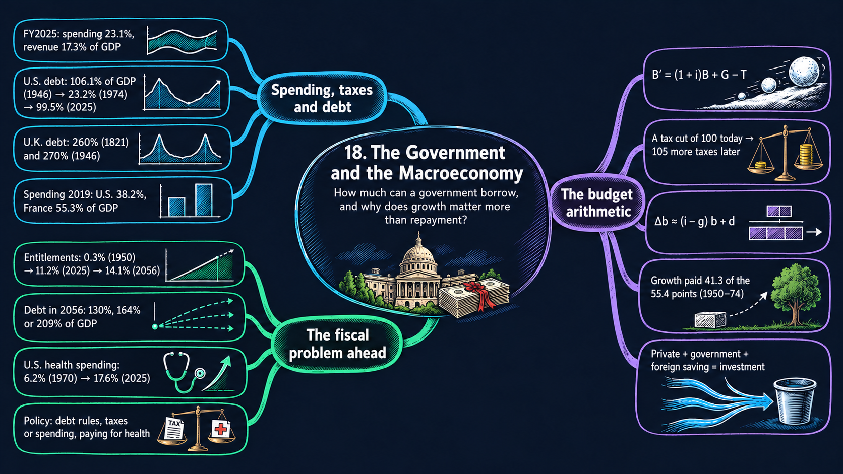
Governments spend between a third and more than half of GDP in the rich countries, and most of them have borrowed a lot. This chapter looks at the data on spending, taxes, deficits and debt, and at the accounting rules that tie them together. By the end of it you will be able to:

• read the U.S. federal budget: where the money goes, where it comes from, and how large the deficit is, in percent of GDP and in dollars per person (Table 18.1);
• derive the flow budget constraint from “uses equal sources”, and use it to compute next year’s debt and the primary and total deficits;
• derive the intertemporal budget constraint by substitution, for two and for more periods, and read its comparative statics: how much a tax cut today raises the taxes of the future;
• derive the law of motion of the debt-GDP ratio with the growth rules, solve for the primary surplus that holds it constant and for its steady state, and state the sustainability conditions (\(i\) below or above \(g\));
• explain why the debt-GDP ratio falls when GDP grows faster than the interest rate, and split the changes in the U.S. ratio into deficits and growth;
• derive the saving-investment identity and use it to measure crowding out;
• compare government spending and debt across countries, and describe the fiscal problem of the twenty-first century: the rise of health spending;
• in Python: write small accounting functions, reshape tables with melt and merge, draw a chart with two vertical axes, animate a bar chart, and compare two vintages of the same data.

Model overview

Islandia has a government now: the Islandia Treasury. Every year it pays for harbor repairs, schools and the coast guard, sends pensions to retired islanders, and owes interest on the bonds it sold in earlier years. Taxes cover most of these bills, and whatever they leave unpaid the Treasury borrows. Can the Treasury keep borrowing year after year, and what decides whether Islandia’s debt stays manageable? This section answers with a few accounting rules that no government can escape, and we follow the Treasury’s books through every step.

NoteThe big idea

The question. How does each year’s deficit turn into debt, and when can a government carry its debt forever without trouble?

The answer in one sentence. Spending must be paid for by taxes now or taxes later, so the budget has to balance in present value, and the debt measured relative to GDP stays stable only if growth and the primary balance keep up with the interest rate.

What goes in and what comes out. We choose spending, taxes, the starting debt, the interest rate and GDP growth. The accounting gives back the deficits, the path of the debt and of the debt-GDP ratio, the taxes the future must raise, and how much investment a deficit displaces.

Road map.

1. The flow budget constraint: uses equal sources in every year, and how the debt rolls forward.
2. The intertemporal budget constraint: chaining the years together, so the budget balances in present value.
3. The debt-GDP ratio and sustainability: how the ratio moves, where it settles, and when it explodes.
4. Saving, investment and crowding out: who pays for new boats when the Treasury borrows.
5. The arithmetic of rising health spending: why the health share of GDP keeps climbing.
6. Model in code: the key relations as Python functions, checked with numbers. The data sections reuse these functions.

Notation. This chapter puts no bars over letters: there is no behavior to solve for, only accounting. Policy choices (spending and taxes) and the rates \(i\) and \(g\) are numbers we set; the debt and the ratios follow from the rules. Capital letters are amounts of money in year \(t\), and lowercase letters are the same amounts divided by GDP. In the code the rates are decimals, so 5 percent is 0.05.

Symbol	Meaning	Type
\(G_t, Tr_t, T_t\)	purchases, transfers and taxes in year \(t\)	parameters
\(i\)	nominal interest rate on the debt, constant	parameter
\(g\)	growth rate of nominal GDP, constant	parameter
\(B_t\)	debt owed at the start of year \(t\)	endogenous
\(\Delta B_{t+1}, \Delta M_{t+1}\)	new bonds sold and new money printed during year \(t\)	endogenous
\(Y_t\)	nominal GDP in year \(t\)	parameter
\(b_t, d_t\)	debt-GDP ratio (end of year \(t\)) and primary deficit ratio	endogenous
\(a\), \(b^*\)	the factor \((1+i)/(1+g)\), and the steady-state debt ratio	endogenous
\(C, I, EX, IM\)	consumption, investment, exports and imports	endogenous
\(\theta, \phi\)	responses of private and foreign saving to a deficit	parameters
\(H, N_r, c, N, y, h\)	health spending, recipients, cost per recipient, population, income per person, health share	endogenous
\(\Delta x_{t+1}\), \(g_x\)	the change \(x_{t+1}-x_t\), and the growth rate of \(x\)	notation

The flow budget constraint

Definitions

Treat the Treasury like a household whose bank account is allowed to go below zero. In each year \(t\) the money goes to three uses:

• purchases of goods and services \(G_t\): on Islandia, harbor repairs, teachers and the coast guard;
• transfers \(Tr_t\), payments that buy nothing in return: pensions for retired islanders, help for those out of work;
• interest on the debt owed at the start of the year, \(iB_t\). The government debt \(B_t\) is the value of the bonds the Treasury sold in the past and has not yet paid back. Islanders, and lenders on Mainland, hold these bonds.

The money comes from three sources:

• taxes \(T_t\);
• new borrowing \(\Delta B_{t+1} \equiv B_{t+1} - B_t\), the value of the bonds sold during the year;
• new money printed by the central bank, \(\Delta M_{t+1}\).

No money appears from nowhere, so the two lists must add up to the same total in every single year.

ImportantKey result: uses equal sources

\[\underbrace{G_t + Tr_t + iB_t}_{\text{uses}} = \underbrace{T_t + \Delta B_{t+1} + \Delta M_{t+1}}_{\text{sources}} \tag{1}\]

Every unit paid out was taxed, borrowed or printed.

We make two simplifications, as the textbook does. First, \(\Delta M_{t+1} = 0\): the Islandia Treasury does not ask the Bank of Islandia to print money for its bills, and neither does the U.S. Treasury (the link between budgets and inflation is the topic of Chapter 8). Second, we put transfers inside \(G_t\), so from here on \(G_t\) is all spending except interest. Neither step changes the logic.

The budget balance is taxes minus spending. A positive balance is a surplus, a negative one is a deficit, and a zero balance means the budget is balanced. Two versions are in use, and they differ only in whether interest counts:

Measure	Formula	Includes interest?
primary deficit	\(G_t - T_t\)	no
total deficit	\(G_t + iB_t - T_t\)	yes

Newspapers and Table 18.1 quote the total deficit. The primary deficit shows what this year’s policy adds to the debt.

Solving the model

Step 1: drop money and transfers. With \(\Delta M_{t+1} = 0\) and \(Tr_t\) inside \(G_t\), equation (1) shrinks to

\[G_t + iB_t = T_t + \Delta B_{t+1}.\]

Step 2: borrowing covers the total deficit. Move \(T_t\) to the left:

\[\Delta B_{t+1} = G_t + iB_t - T_t.\]

Each unit of total deficit is matched by one unit of new bonds.

Step 3: next year’s debt. Write \(\Delta B_{t+1} = B_{t+1} - B_t\) and add \(B_t\) to both sides:

\[B_{t+1} = B_t + iB_t + G_t - T_t.\]

The two terms in \(B_t\) combine, \(B_t + iB_t = (1+i)B_t\), and give the law of motion of the debt in the box below.

ImportantKey result: the flow budget constraint

\[B_{t+1} = (1+i)B_t + \underbrace{G_t - T_t}_{\text{primary deficit}} \tag{2}\]

Next year’s debt is this year’s debt plus interest, plus the primary deficit.

Islandia in numbers. Take the case used in the code checks: the Treasury owes \(B_t = 5\) (in billions), pays \(i = 0.05\), and spends and taxes \(G_t = T_t = 4\). The primary deficit is zero, the total deficit is the interest bill \(0.05 \times 5 = 0.25\), and next year’s debt is \(1.05 \times 5 = 5.25\).

TipIn words

Islandia’s debt behaves like an unpaid credit-card balance. Each year interest is charged on the old balance, and any spending beyond taxes is added on top. Even when taxes cover spending, the debt grows, because the interest itself is borrowed.

What the model predicts

Equation (2) tells us how fast the debt grows under any policy. Divide it by \(B_t\):

\[\frac{\Delta B_{t+1}}{B_t} = i + \frac{G_t - T_t}{B_t}.\]

Policy	Primary deficit	Total deficit	Growth rate of the debt
primary budget balanced, \(T_t = G_t\)	\(0\)	\(iB_t\)	\(i\)
total budget balanced, \(T_t = G_t + iB_t\)	\(-iB_t\) (a surplus)	\(0\)	\(0\)
primary deficit \(G_t - T_t > 0\)	positive	larger than \(iB_t\)	above \(i\)

• One more unit of primary deficit adds exactly one unit to next year’s debt. One more point of interest adds \(0.01\,B_t\).
• With a balanced primary budget, taxes pay for current spending but not for the interest. The interest is borrowed, so the debt grows at the rate \(i\).
• To keep the debt from growing at all, the Treasury needs a primary surplus as large as its interest bill.

The debt grows by the interest on the old debt plus the primary deficit; stopping it takes a primary surplus that covers interest.

NoteCheck your understanding

1. The Treasury owes 5 billion at 5 percent interest and spends 4 billion. How large must taxes be to keep the debt at exactly 5 billion next year?

Answer

By equation (2), the debt stays put when \(G_t - T_t = -iB_t\), a primary surplus equal to the interest bill of \(0.05 \times 5 = 0.25\). So taxes must be \(4 + 0.25 = 4.25\) billion. The total budget is then balanced.

The intertemporal budget constraint

Assumptions

• The economy lasts two periods, 1 and 2. Think of period 1 as “now” and period 2 as “all the years to come”.
• The Treasury enters period 1 owing \(B_1\), which may be positive (the United States, like many countries, starts with a large debt).
• Equation (2) holds in both periods, with the same interest rate \(i\).
• After period 2 nobody will lend to the Treasury, because there is no later period in which a loan could be repaid. So the debt left over at the start of period 3 must be zero: \(B_3 = 0\).

Solving the model

Step 1: the two flow constraints. Write equation (2) for \(t = 1\) and for \(t = 2\):

\[B_2 = (1+i)B_1 + G_1 - T_1 \qquad\text{and}\qquad 0 = B_3 = (1+i)B_2 + G_2 - T_2.\]

Step 2: solve the second one for \(B_2\). Move \(G_2 - T_2\) to the left and divide by \(1+i\):

\[B_2 = \frac{T_2 - G_2}{1+i}.\]

The debt carried into period 2 equals the period-2 surplus, in period-1 money.

Step 3: substitute into the first one. Replace \(B_2\) in the period-1 constraint:

\[\frac{T_2 - G_2}{1+i} = (1+i)B_1 + G_1 - T_1.\]

Step 4: sort spending and taxes. Split the fraction, \(\frac{T_2 - G_2}{1+i} = \frac{T_2}{1+i} - \frac{G_2}{1+i}\). Then collect the spending terms and the debt on the left and the tax terms on the right:

\[G_1 + \frac{G_2}{1+i} + (1+i)B_1 = T_1 + \frac{T_2}{1+i}.\]

Dividing a period-2 amount by \(1+i\) gives its present discounted value (pdv): the sum that, lent out now at the rate \(i\), would grow into that amount by period 2 (Appendix C.12). The starting debt carries the factor \(1+i\) because its period-1 interest is due as well.

Step 5: the same result in budget balances. Move \(G_1\) and \(G_2/(1+i)\) to the right and combine the terms of each period:

\[(T_1 - G_1) + \frac{T_2 - G_2}{1+i} = (1+i)B_1.\]

ImportantKey result: the intertemporal budget constraint

\[\underbrace{G_1 + \frac{G_2}{1+i}}_{\text{pdv of spending}} + \underbrace{(1+i)B_1}_{\text{initial debt}} = \underbrace{T_1 + \frac{T_2}{1+i}}_{\text{pdv of taxes}} \tag{3}\]

\[\underbrace{(T_1 - G_1)}_{\text{period-1 balance}} + \underbrace{\frac{T_2 - G_2}{1+i}}_{\text{period-2 balance}} = \underbrace{(1+i)B_1}_{\text{initial debt}} \tag{4}\]

Spending plus the starting debt equals taxes, all in present value.

Islandia in numbers. In the code’s example the Treasury starts owing \(B_1 = 25\), spends 7 in each period and taxes 5 in period 1, with \(i = 0.05\). Equation (2) gives \(B_2 = 1.05 \times 25 + 7 - 5 = 28.25\), and repaying everything in period 2 takes taxes of \(T_2 = 1.05 \times 28.25 + 7 \approx 36.66\).

TipIn words

Equation (3) is “uses equal sources” again, summed over all periods in present value. Equation (4) says it through the balances: a deficit in one period needs a surplus of the same present value in another. Because Islandia already owes money, its surpluses must be bigger still, big enough to pay that debt off.

Step 6: more periods. The argument never used the fact that there are two periods. With three periods and \(B_4 = 0\), solve the period-3 constraint for \(B_3 = (T_3 - G_3)/(1+i)\), put it into the period-2 constraint, and solve that for \(B_2\):

\[B_2 = \frac{T_2 - G_2}{1+i} + \frac{T_3 - G_3}{(1+i)^2}.\]

Substituting this into the period-1 constraint and sorting the terms as in step 4 gives

\[G_1 + \frac{G_2}{1+i} + \frac{G_3}{(1+i)^2} + (1+i)B_1 = T_1 + \frac{T_2}{1+i} + \frac{T_3}{(1+i)^2}.\]

Each extra period adds one more term, discounted one more time. With \(N\) periods, an amount of period \(t\) is divided by \((1+i)^{t-1}\).

What the model predicts

Solve equation (3) for the taxes of period 2:

\[T_2 = (1+i)\big[(1+i)B_1 + G_1 - T_1\big] + G_2.\]

Holding every other term fixed, this formula gives the comparative statics:

A one-dollar rise in …	changes \(T_2\) by	Why
period-1 taxes \(T_1\) (a tax cut is a fall)	\(-(1+i)\)	a dollar not taxed today is borrowed and repaid with interest
period-1 spending \(G_1\)	\(+(1+i)\)	the same: it is financed by borrowing
period-2 spending \(G_2\)	\(+1\)	paid in the same period
the initial debt \(B_1\)	\(+(1+i)^2\)	it accumulates interest over two periods

• A tax cut now is a tax rise later. With \(i = 5\%\), cutting taxes by 100 today while spending stays the same calls for 105 more in taxes in period 2.
• The Treasury can move taxes in time, but not shrink their present value. Given spending and the starting debt, equation (3) pins down the pdv of taxes. A tax cut now only pushes taxes into the future. If islanders see this coming and save their tax cut to pay the later taxes, they consume exactly as before. This is Ricardian equivalence, which comes from the permanent-income theory of consumption (Chapter 16).
• Generational accounting. When period 2 lies far ahead, the islanders who pay the later taxes are not the ones who enjoyed the earlier spending. A rising debt moves tax burdens onto future generations: perhaps fairly, as when a war fought now also protects them, but it is a transfer all the same.

Borrowing never removes a tax: it only moves it to the future, with interest.

NoteCheck your understanding

1. In the example of the Key result, the Treasury cuts period-1 taxes from 5 to 4 and keeps spending unchanged. What must period-2 taxes be now?

Answer

By the comparative statics of equation (3), a one-unit tax cut in period 1 raises \(T_2\) by \(1+i = 1.05\). So \(T_2\) rises from about 36.66 to about 37.71. Check it with equation (2): \(B_2 = 1.05 \times 25 + 7 - 4 = 29.25\), and \(T_2 = 1.05 \times 29.25 + 7 \approx 37.71\).

2. Islanders look ahead and save every unit of that tax cut. Does their consumption in period 1 change?

Answer

No. Equation (3) fixes the present value of their taxes, so the cut today is matched, in present value, by the higher taxes of period 2. Saving the cut, with interest, pays exactly for those later taxes. This is Ricardian equivalence.

The debt-GDP ratio and sustainability

Definitions

How much the Treasury can borrow depends on how much it can later tax, and the best measure of what it can tax is Islandia’s GDP. So we divide every amount by nominal GDP \(Y_t\):

• the debt-GDP ratio \(b_t \equiv B_{t+1}/Y_t\): the debt at the end of year \(t\) (which is the debt owed at the start of year \(t+1\)) over that year’s GDP. Statistical tables, and the data in Figs. 2 and 4, report the ratio this way;
• the primary deficit ratio \(d_t \equiv (G_t - T_t)/Y_t\). A negative \(d_t\) means a primary surplus;
• the growth rate of nominal GDP, \(g\), so that \(Y_t = (1+g)Y_{t-1}\).

Both \(i\) and \(g\) are nominal rates: inflation is inside both.

Solving the model

Step 1: divide the flow constraint by GDP. Divide each term of equation (2) by \(Y_t\):

\[\frac{B_{t+1}}{Y_t} = (1+i)\frac{B_t}{Y_t} + \frac{G_t - T_t}{Y_t}.\]

The left side is \(b_t\), and the last term is \(d_t\).

Step 2: rewrite the middle term. \(B_t\) is the debt at the end of year \(t-1\), yet here it is divided by this year’s GDP. Multiply and divide by \(Y_{t-1}\):

\[\frac{B_t}{Y_t} = \frac{B_t}{Y_{t-1}}\cdot\frac{Y_{t-1}}{Y_t} = b_{t-1}\cdot\frac{1}{1+g}.\]

Step 3: the law of motion of the ratio. Put step 2 into step 1:

\[b_t = \frac{1+i}{1+g}\,b_{t-1} + d_t.\]

This holds exactly. It is a difference equation: it gives this year’s ratio from last year’s (Appendix C.10).

Step 4: the change in the ratio. Subtract \(b_{t-1}\) from both sides and use \(\frac{1+i}{1+g} - 1 = \frac{(1+i) - (1+g)}{1+g} = \frac{i-g}{1+g}\):

\[b_t - b_{t-1} = \frac{i-g}{1+g}\,b_{t-1} + d_t \;\approx\; (i-g)\,b_{t-1} + d_t.\]

The approximation drops the division by \(1+g\), which is close to 1 when \(g\) is a few percent (Appendix C.6).

ImportantKey result: the law of motion of the debt-GDP ratio

\[b_t = \frac{1+i}{1+g}\,b_{t-1} + d_t \tag{5}\]

\[b_t - b_{t-1} = \frac{i-g}{1+g}\,b_{t-1} + d_t \;\approx\; (i-g)\,b_{t-1} + d_t \tag{6}\]

The ratio rises with the primary deficit, and with the gap between the interest rate and growth times the debt already owed.

TipIn words

Two forces move Islandia’s ratio. The primary deficit adds fresh debt. And the old debt is a race: interest pushes it up at the rate \(i\), while GDP, the denominator, grows at the rate \(g\). When \(g\) is larger than \(i\), Islandia simply outgrows its debt.

The growth rule for a ratio, \(g_b = g_B - g_Y\) (Appendix C.5), agrees. With a balanced primary budget the debt grows at \(i\), so the ratio grows at about \(i - g\). With a balanced total budget the debt stays put, so the ratio shrinks at about the rate \(g\).

Step 5: the primary balance that holds the ratio constant. Set \(b_t = b_{t-1} = b\) in the exact form of equation (6) and solve for the primary surplus \(-d\):

\[-d = \frac{i-g}{1+g}\,b.\]

When \(i > g\), holding the ratio still takes a primary surplus, larger the more a country owes. When \(i < g\), it can run a primary deficit forever and still hold the ratio constant.

Step 6: the long-run ratio and the path toward it. Let the primary deficit ratio stay at the same value \(d\) every year, and write \(a \equiv (1+i)/(1+g)\). A steady state \(b^*\) is a ratio that repeats itself, \(b^* = a\,b^* + d\). Collect the \(b^*\) terms, \(b^*(1-a) = d\), and use \(1 - a = \frac{g-i}{1+g}\):

\[b^* = \frac{1+g}{g-i}\,d.\]

Now subtract \(b^* = a b^* + d\) from equation (5). The \(d\) cancels and leaves \(b_t - b^* = a\,(b_{t-1} - b^*)\): every year the gap to \(b^*\) is multiplied by \(a\). After \(t\) years it has been multiplied by \(a^t\):

\[b_t = b^* + \left(\frac{1+i}{1+g}\right)^{t}\,(b_0 - b^*).\]

ImportantKey result: the stabilizing surplus and the path of the ratio

\[-d = \frac{i-g}{1+g}\,b \tag{7}\]

\[b_t = b^* + \left(\frac{1+i}{1+g}\right)^{t}\,(b_0 - b^*), \qquad b^* = \frac{1+g}{g-i}\,d \tag{8}\]

Equation (7) is the primary surplus that keeps the ratio still. Equation (8) gives the whole path for a constant primary deficit.

Islandia in numbers. Give Islandia the chapter’s debt ratio of 99.5 percent of GDP. With \(i = g\) it needs no primary surplus at all. With \(i = 0.05\) and \(g = 0.04\) it needs a primary surplus of \(0.01/1.04 \times 99.5 \approx 0.96\) percent of GDP every year. With \(i = 0.03\), \(g = 0.04\) and a primary deficit of 2 percent of GDP forever, the ratio heads for \(b^* = 1.04/0.01 \times 2 = 208\) percent, slowly: \(a = 1.03/1.04 \approx 0.990\), so the gap closes by only about 1 percent a year.

What the model predicts

Sustainability conditions. Everything hinges on whether \(a = (1+i)/(1+g)\) is below or above one, that is, on whether \(i\) is below or above \(g\):

Case	What \(a^t\) does	What happens to the debt ratio
\(i < g\)	shrinks to 0	converges to \(b^*\) from any start. A constant primary deficit gives a finite ratio, even though the dollar debt grows forever.
\(i = g\)	stays at 1	\(b_t = b_{t-1} + d_t\): the ratio is the starting ratio plus the sum of all later primary deficits. It is stable only if primary deficits and surpluses cancel.
\(i > g\)	grows without limit	\(b^*\) is a tipping point, not a resting point. Above it the ratio explodes, below it the ratio falls. Only primary surpluses of at least equation (7) keep the ratio from rising.

The ratio of 99.5 percent is the U.S. debt held by the public in FY2025, and \(i = g = 4\%\) are the starting values of the projection widget in Fig. 6.

Comparative statics of equation (6). Holding last year’s ratio fixed:

A one-point rise in …	changes this year’s \(b_t - b_{t-1}\) by about	With \(b_{t-1} = 99.5\%\)
the primary deficit \(d_t\) (% of GDP)	\(+1\) point	\(+1\) point
the interest rate \(i\)	\(+b_{t-1}/100\) points	\(+1\) point
nominal GDP growth \(g\)	\(-b_{t-1}/100\) points	\(-1\) point

Near 100 percent of GDP, one point of interest weighs as much as one point of primary deficit. The higher the debt, the more the ratio responds to \(i\) and \(g\).

Growth is a powerful remedy. The ratio can fall a long way with no repayment at all, as long as GDP grows faster than the interest rate. This is mostly how the U.S. ratio came down after World War II (Fig. 2).

Inflation, expected and unexpected. Write \(1+i = (1+r)(1+\pi)\) and \(1+g = (1+g_{\text{real}})(1+\pi)\), with \(r\) the real interest rate, \(g_{\text{real}}\) real GDP growth and \(\pi\) inflation (the Fisher equation, Chapter 8). The inflation factor cancels in \(a\):

\[\frac{1+i}{1+g} = \frac{1+r}{1+g_{\text{real}}}.\]

Expected inflation is already priced into \(i\), so it leaves the ratio alone. Surprise inflation, after the bonds were sold at a fixed \(i\), cuts the real rate paid and erodes the debt. Hence very large debts raise fears of inflation.

Confidence and default. Lenders who doubt repayment demand a higher \(i\) on new bonds. That raises \(a\) and the surplus of equation (7), and can turn a stable ratio into an explosive one. The fear can fulfill itself and end in high inflation or a default. No single ratio sets off a crisis: it depends on the outlook for growth, on how well the government collects taxes, and on how much lenders trust it.

A debt is sustainable when growth outruns the interest rate, or when primary surpluses make up the difference.

NoteCheck your understanding

1. Islandia’s debt is 99.5 percent of GDP and nominal GDP grows at 4 percent. Lenders grow nervous and the interest rate rises to 6 percent. What primary surplus now keeps the ratio constant?

Answer

By equation (7), \(-d = (0.06 - 0.04)/1.04 \times 99.5 \approx 1.91\) percent of GDP a year, twice the surplus needed at an interest rate of 5 percent. A loss of confidence makes the debt harder to carry.

2. The Bank of Islandia lets inflation rise by surprise, after the Treasury has sold its bonds at a fixed interest rate. Why does the debt ratio fall? Would the same rise in inflation help if lenders had expected it?

Answer

The surprise raises nominal GDP growth \(g\) while the interest rate on the old bonds stays fixed, so \((1+i)/(1+g)\) falls and the ratio in equation (5) shrinks. Expected inflation would already be built into \(i\), raising \(i\) and \(g\) together, so the factor \((1+r)/(1+g_{\text{real}})\) and the ratio would not change.

Saving, investment and crowding out

Definitions

The national income identity of Chapter 2 splits GDP by how it is used: \(Y = C + I + G + EX - IM\). Here \(G\) means government purchases only; we leave transfers out to keep the algebra short. With taxes \(T\) there are three kinds of saving:

• private saving \(Y - T - C\): the part of disposable income, \(Y - T\), that islanders and firms do not consume;
• government saving \(T - G\): the Treasury’s budget balance;
• foreign saving \(IM - EX\): when Islandia buys more from Mainland than it sells there, Mainland lends it the difference.

Solving the model

Step 1: solve the identity for investment. Subtract \(C\), \(G\) and \(EX - IM\) from both sides of \(Y = C + I + G + EX - IM\):

\[I = Y - C - G + (IM - EX).\]

Step 2: add and subtract taxes. Adding \(-T + T = 0\) leaves the equation as it was, but lets us group the terms by who does the saving:

\[I = (Y - T - C) + (T - G) + (IM - EX).\]

Put saving on the left, and the identity is the first equation in the box below.

Step 3: a larger deficit. Let the deficit rise by \(\Delta\), so government saving falls by \(\Delta\). Suppose private saving responds by \(\theta\Delta\) and foreign saving by \(\phi\Delta\). The change in investment is the sum of the changes in the three kinds of saving:

\[\Delta I = \theta\Delta - \Delta + \phi\Delta.\]

ImportantKey result: the saving-investment identity and crowding out

\[\underbrace{(Y-T-C)}_{\text{private saving}} + \underbrace{(T-G)}_{\text{government saving}} + \underbrace{(IM-EX)}_{\text{foreign saving}} = I \tag{9}\]

\[\Delta I = \theta\Delta - \Delta + \phi\Delta = -(1 - \theta - \phi)\,\Delta \tag{10}\]

Investment falls by the part of a deficit that other saving does not make up.

Islandia in numbers. In the code’s example, in percent of GDP: \(C = 67\), \(I = 18\), \(G = 20\), \(EX = 11\), \(IM = 16\) and \(T = 17\). Private saving is \(100 - 17 - 67 = 16\), government saving is \(17 - 20 = -3\), foreign saving is \(16 - 11 = 5\), and together they make \(16 - 3 + 5 = 18 = I\).

TipIn words

Every new boat that Harbor Boatworks buys has to be paid for with someone’s saving: the islanders’, the Treasury’s, or Mainland’s. A deficit is negative saving by the Treasury, so it draws on the saving of the other two. Unless islanders save more or Mainland lends more, less is left for boats.

What the model predicts

Response of other saving	\(\theta\)	\(\phi\)	Change in investment
none (full crowding out)	0	0	\(-\Delta\)
Ricardian equivalence: households save the whole tax cut	1	0	\(0\)
private saving offsets half	0.5	0	\(-0.5\Delta\)
half from households, the rest from foreigners	0.5	0.5	\(0\)

The evidence suggests that private saving rises by at most about half of a deficit. So without help from abroad, at least half of a deficit would come out of investment. Foreign saving can cover the rest, as Fig. 5 suggests it did in the United States. The foreign side is the topic of Chapter 19.

A deficit is paid for by more private saving, more foreign lending, or less investment.

NoteCheck your understanding

1. The Treasury’s deficit rises by 2 percent of GDP. Islanders save a quarter of it (\(\theta = 0.25\)) and Mainland lends another quarter (\(\phi = 0.25\)). By how much does investment change?

Answer

By equation (10), \(\Delta I = -(1 - 0.25 - 0.25) \times 2 = -1\): investment falls by 1 percent of GDP. Half of the deficit is crowded out.

2. Why does Ricardian equivalence imply no crowding out at all?

Answer

If islanders expect the tax cut to be paid back with higher taxes later (equation 3), they save all of it, so \(\theta = 1\). Private saving rises exactly as much as government saving falls, and by equation (10) investment does not change.

The arithmetic of rising health spending

Definitions

Long-run budget projections are driven by entitlement programs, above all public health spending. Split both health spending and GDP into two pieces:

• health spending \(H = N_r \times c\): the number of people who receive benefits, \(N_r\), times the cost per recipient, \(c\);
• GDP \(Y = N \times y\): the population \(N\) times GDP per person \(y\);
• the health share \(h \equiv H/Y\).

Solving the model

Step 1: the share as a product of two ratios. Divide and regroup:

\[h = \frac{N_r\,c}{N\,y} = \frac{N_r}{N}\times\frac{c}{y}.\]

The share is the fraction of the population that receives benefits, times the cost per recipient relative to income per person.

Step 2: take growth rates. The growth rate of a product is the sum of the growth rates, and the growth rate of a ratio is the difference (Appendix C.5). Applied to step 1, this gives the result in the box.

ImportantKey result: the growth of the health share

\[g_h = g_{N_r/N} + (g_c - g_y) \tag{11}\]

The share grows with the share of recipients and with costs that outpace income.

Islandia in numbers. As in the code’s check, let the cost of care per recipient grow 3 percent a year and income per person 2 percent, with a constant share of recipients. The health share then grows by about 1 percent a year (exactly \(1.03/1.02 - 1 \approx 0.98\) percent) and roughly doubles in 70 years, from 5 to about 9.9 percent of GDP.

TipIn words

Islandia is aging: each year a slightly larger share of islanders draws on public health care. And care gets more expensive faster than incomes rise. Each force adds its own growth rate to the health share, even when the programs never change.

What the model predicts

• Aging raises the share through \(g_{N_r/N}\): fewer workers per retiree means more recipients per person.
• Costs that outpace income raise it through \(g_c - g_y\). If the cost per recipient grows just 1 point a year faster than income per person, the share grows by about 1 percent a year and doubles in about 70 years (the rule of 70). Add an aging effect of another 1 percent a year and it doubles in about 35 years.
• The budget link. The primary deficit ratio is non-interest spending minus revenue, both in percent of GDP. If revenue stays near a fixed share of GDP while \(h\) keeps climbing, \(d_t\) rises every year and equation (5) pushes the debt ratio up without limit. Either taxes go up or spending comes down.
• Why the share may keep rising. As people get richer, an extra unit of consumption adds less and less to their well-being (diminishing marginal utility), while an extra year of life to enjoy it keeps its value. So standard models predict health spending growing faster than income. The problem is less waste than how to pay for spending people want.

Aging and costs that outpace income make the health share grow, and the budget must eventually pay for it.

NoteCheck your understanding

1. On Islandia the cost per recipient grows 3 percent a year, income per person 2 percent, and the share of recipients 1 percent. About how fast does the health share grow, and in about how many years does it double?

Answer

By equation (11), \(g_h \approx 1 + (3 - 2) = 2\) percent a year. By the rule of 70, the share doubles in about \(70/2 = 35\) years.

2. The Treasury keeps revenue at a fixed share of GDP while the health share rises. What happens to the debt ratio, even if \(i = g\)?

Answer

The primary deficit ratio \(d_t\) rises every year. With \(i = g\), equation (5) becomes \(b_t = b_{t-1} + d_t\), so the ratio adds up ever larger deficits and keeps climbing. Only higher taxes or lower spending elsewhere can stop it.

NoteRecap

• Uses equal sources every year: the debt rolls forward as \(B_{t+1} = (1+i)B_t + G_t - T_t\), and the deficits of each year add up to the debt (U.S. debt data).
• The budget balances in present value: spending plus the starting debt equals taxes in pdv, so a tax cut today means higher taxes later.
• The debt-GDP ratio moves with the primary deficit and with \(i - g\) times the old debt. Growth faster than interest shrinks it, as after World War II (Fig. 2: primary deficits and growth).
• Sustainability: with \(i < g\) the ratio settles at \(b^*\); with \(i > g\) only primary surpluses stop it from exploding (Fig. 6).
• Crowding out: a deficit lowers investment unless private or foreign saving makes up for it (Fig. 5 in numbers).
• Health spending grows faster than GDP when the population ages and costs outpace income, the fiscal problem of this century (why health spending rises).

Model in code

Now we turn the Key results into Python. The section has four parts: the setup (folded, because it is the same in every chapter), the budget rules as functions, numerical checks of the Key results, and the drawing and data tools that the figures use (folded too). Run its cells once, in order. Every later section of the notebook reuses them.

Setup

Run the setup cells once, before anything else. They load the Python libraries, give every chart the same look, store the address of the chapter’s data and define a helper that only the book website needs. You can use the notebook without reading them; open the box if you are curious.

NoteShow the setup code

The first cell loads the libraries and sets the look of the charts. Its comments explain each step.

# @title Setup: libraries, chart colors and the data location
# Text after a "#" is a comment: Python ignores it, it is there for human readers.

# Step 1: load the libraries. `import` loads a library, a toolbox written by
# other people, and `as np` gives it a short nickname, so the code stays short.
import numpy as np                    # numbers and arrays
import pandas as pd                   # data tables
import plotly.express as px           # quick charts from data tables
import plotly.graph_objects as go     # charts built piece by piece
import plotly.io as pio               # settings shared by every chart
# menus, buttons and sliders for the interactive figures
from ipywidgets import interact, Dropdown, ToggleButtons, FloatSlider, SelectMultiple, fixed

# Step 2: one light blue/green look for every chart
BLUE, TEAL, GREEN, GRAY = "#16528c", "#008070", "#7fb23a", "#8a96a3"
# extra colors for the five-country charts
LIGHT_BLUE, DARK_TEAL, ORANGE = "#5aa0d8", "#0b4f47", "#e0a33b"
pio.templates.default = "plotly_white"
# the same chart size in Colab and on the website
pio.templates["plotly_white"].layout.update(width=860, height=480)
px.defaults.color_discrete_sequence = [BLUE, TEAL, GREEN, LIGHT_BLUE, DARK_TEAL]
WIDE = {"description_width": "initial"}         # show the full widget labels

# Step 3, Colab only: let Plotly charts appear inside the interactive widgets.
# `try` runs the indented lines; if the import fails (we are not in Colab),
# `except` skips them.
try:
    import google.colab
    google.colab.output.enable_custom_widget_manager()
except ImportError:
    pass                                        # not running in Colab: nothing to do

# Step 4: the data files of this chapter live in the book's GitHub repository
DATA_URL = "https://raw.githubusercontent.com/quarcs-lab/macro102-site/main/data/ch18/"

The website cannot run Python, so each interactive figure also gets a version with a precomputed slider. The next helper builds those versions. Run it and move on.

# @title Helper for the website versions (run this cell; you do not need to read it)
def slider_figure(make_figure, name, values, start, label=None):
    """Join precomputed versions of a figure with one slider (the website cannot run Python).

    Arguments
        make_figure : the function that draws the figure
        name        : the argument the slider moves
        values      : the values of that argument to precompute
        start       : the value shown first
        label       : the slider's label (the argument name if None)
    Returns
        one Plotly figure with all versions and a slider that shows one at a time
    """
    # Step 1: draw the figure once for every value
    figures = [make_figure(**{name: v}) for v in values]
    first = values.index(start)
    # Step 2: copy every curve into one figure; only the start value's are visible
    fig = go.Figure(layout=figures[first].layout)
    owner = []                          # which precomputed figure each trace is from
    for i, f in enumerate(figures):
        for trace in f.data:
            trace.visible = (i == first)
            fig.add_trace(trace)
            owner.append(i)
    # Step 3: one slider step per value: its curves, title, labels and shapes
    steps = []
    for i, f in enumerate(figures):
        layout = {"title": f.layout.title.to_plotly_json(),
                  "annotations": [a.to_plotly_json() for a in f.layout.annotations],
                  "shapes": [s.to_plotly_json() for s in f.layout.shapes]}
        visible = [o == i for o in owner]
        steps.append(dict(method="update", label=str(values[i]), args=[{"visible": visible}, layout]))
    fig.update_layout(sliders=[dict(active=first, steps=steps, pad=dict(t=60),
                                    currentvalue=dict(prefix=(label or name) + " = "))])
    return fig

The model as functions

The Key results are accounting rules, so each one becomes a short Python function: a named recipe that takes inputs and gives back a result. The first four follow the Treasury’s books in money: the flow constraint, equation (2), the two deficits and the present value of equation (3).

# `def` creates a function. Its inputs are the arguments in parentheses.
# The text in triple quotes describes the function. Rates are decimals: 5% is 0.05.
def next_debt(B, G, T, i):
    """Next period's debt, from the flow budget constraint.

    Equation (2):  B_{t+1} = (1 + i) B_t + G_t - T_t

    Arguments
        B : debt at the start of the period, B_t
        G : spending except interest, G_t
        T : taxes, T_t
        i : nominal interest rate on the debt
    Returns
        the debt at the start of the next period, B_{t+1}
    """
    # `return` gives back the result: old debt with interest, plus the primary deficit
    return (1 + i) * B + G - T


def primary_deficit(G, T):
    """Primary deficit: spending minus taxes, leaving out the interest payments.

    Equation (2), its last term:  primary deficit = G_t - T_t

    Arguments
        G : spending except interest, G_t
        T : taxes, T_t
    Returns
        the primary deficit (negative for a primary surplus)
    """
    # interest on the debt is left out
    return G - T


def total_deficit(G, T, i, B):
    """Total deficit: spending plus the interest on the debt, minus taxes.

    Equation (2), rearranged:  total deficit = G_t + i B_t - T_t = B_{t+1} - B_t

    Arguments
        G : spending except interest, G_t
        T : taxes, T_t
        i : nominal interest rate on the debt
        B : debt at the start of the period, B_t
    Returns
        the total deficit, the number newspapers quote
    """
    # the primary deficit plus this year's interest bill i B
    return G + i * B - T


def pdv(first, second, i):
    """Present discounted value of an amount in period 1 and one in period 2.

    Equation (3), each side:  pdv = first + second / (1 + i)

    Arguments
        first  : the amount in period 1
        second : the amount in period 2
        i      : nominal interest rate, used to discount period 2
    Returns
        the present discounted value, in period-1 money
    """
    # an amount in period 2 is worth 1 / (1 + i) of it today
    return first + second / (1 + i)

Next come the rules for the debt-GDP ratio. next_debt_ratio is equation (5), and debt_ratio_path applies it year after year. debt_change_parts splits a change in the ratio in two, as equation (6) does.

def next_debt_ratio(b, i, g, d):
    """Next year's debt-GDP ratio.

    Equation (5):  b_t = (1 + i) / (1 + g) b_{t-1} + d_t

    Arguments
        b : last year's debt ratio, b_{t-1} (percent of GDP)
        i : nominal interest rate on the debt
        g : growth rate of nominal GDP
        d : this year's primary deficit, d_t (percent of GDP)
    Returns
        this year's debt ratio, b_t (percent of GDP)
    """
    # the old ratio grows by the factor a = (1 + i) / (1 + g), then d adds to it
    return (1 + i) / (1 + g) * b + d


def debt_ratio_path(b, i, g, deficits):
    """The debt ratio after each year of a list of primary deficits.

    Equation (5), applied once a year:  b_t = (1 + i) / (1 + g) b_{t-1} + d_t

    Arguments
        b        : the starting debt ratio, b_0 (percent of GDP)
        i        : nominal interest rate on the debt
        g        : growth rate of nominal GDP
        deficits : the primary deficit of each year, d_1, d_2, ... (percent of GDP)
    Returns
        a list with the debt ratio at the end of each year
    """
    # Step 1: `path = []` starts an empty list
    path = []
    # Step 2: the `for` loop runs its indented lines once for each deficit in the
    # list; each pass replaces b by next year's ratio, and `path.append(b)` adds
    # it at the end of the list
    for d in deficits:
        b = next_debt_ratio(b, i, g, d)
        path.append(b)
    return path


def debt_change_parts(debt, deficit, start, end):
    """Split the change in the debt ratio from start to end into primary deficits and the rest.

    Equation (6), summed over the years:  b_end - b_start = sum of d_t + sum of (i - g) / (1 + g) b_{t-1}

    Arguments
        debt    : the debt ratio, a Series with years as row labels
        deficit : the primary deficit ratio, a Series with years as row labels
        start   : the first year
        end     : the last year
    Returns
        the change in the ratio, the part from primary deficits, and the rest (interest minus growth)
    """
    # Step 1: the change in the ratio over the whole period
    change = debt[end] - debt[start]
    # Step 2: `.loc[start + 1:end]` keeps the years start + 1 to end (both included),
    # and `.sum()` adds up their primary deficits
    from_deficits = deficit.loc[start + 1:end].sum()
    # Step 3: what deficits do not explain is the interest-minus-growth term
    return change, from_deficits, change - from_deficits

The part of a change that is not explained by primary deficits, change - from_deficits, is the effect of interest minus growth, the term \(\frac{i-g}{1+g}\,b\) of equation (6), summed over the years. We use it on the U.S. data in Fig. 2. Three more functions give the long-run results of the debt ratio and the saving identity.

def stabilizing_surplus(b, i, g):
    """The primary surplus that keeps the debt ratio constant.

    Equation (7):  -d = (i - g) / (1 + g) b

    Arguments
        b : the debt ratio to hold (percent of GDP)
        i : nominal interest rate on the debt
        g : growth rate of nominal GDP
    Returns
        the stabilizing primary surplus, -d (percent of GDP)
    """
    # the surplus pays just the part of the interest that growth does not cover
    return (i - g) / (1 + g) * b


def steady_state_ratio(d, i, g):
    """The steady-state debt ratio for a constant primary deficit.

    Equation (8):  b* = (1 + g) / (g - i) d

    Arguments
        d : the constant primary deficit (percent of GDP; negative for a surplus)
        i : nominal interest rate on the debt
        g : growth rate of nominal GDP
    Returns
        the steady-state debt ratio, b* (percent of GDP)
    """
    # with i < g the ratio settles here; with i > g it is a tipping point
    return (1 + g) / (g - i) * d


def private_and_foreign_saving(investment, government_saving):
    """The saving of households, firms and foreigners that investment needs.

    Equation (9), solved for private plus foreign saving:  (Y - T - C) + (IM - EX) = I - (T - G)

    Arguments
        investment        : investment, I
        government_saving : government saving, T - G
    Returns
        private plus foreign saving
    """
    # whatever the government does not save, others must save for investment
    return investment - government_saving

Checking the key results

The formulas came from algebra. Now we check them with numbers, one Key result at a time.

Check 1: the flow constraint, with Exercise 5 of the textbook. A government owes 5 trillion dollars at an interest rate of 5 percent, and GDP (20 trillion dollars) grows by 4 percent a year. In case (a) it balances its primary budget (\(G = T\)). In case (b) it balances its total budget, so taxes also pay the interest.

# Step 1: the rates, and the starting debt and GDP
i, g = 0.05, 0.04                      # interest rate and GDP growth rate
# debt in cases (a) and (b), and GDP, trillions of dollars
B_a, B_b, Y = 5.0, 5.0, 20.0
# Step 2: follow both cases for three years. An f-string, f"... {value:.3f}",
# puts a value into the text; ":.3f" means "three decimals".
for year in [1, 2, 3]:
    # case (b): taxes cover spending of 4.0 and the interest
    T_b = 4.0 + i * B_b
    print(f"Year {year}: (a) primary deficit {primary_deficit(4.0, 4.0):.2f}, total {total_deficit(4.0, 4.0, i, B_a):.3f}"
          f"   (b) primary deficit {primary_deficit(4.0, T_b):.2f}, total {total_deficit(4.0, T_b, i, B_b):.2f}")
    # equation (2): the new debt replaces the old one in each case
    B_a = next_debt(B_a, G=4.0, T=4.0, i=i)
    B_b = next_debt(B_b, G=4.0, T=T_b, i=i)
    Y = (1 + g) * Y                    # GDP grows by g
    print(f"   debt (a) {B_a:.3f} = {100 * B_a / Y:.2f}% of GDP,  debt (b) {B_b:.3f} = {100 * B_b / Y:.2f}% of GDP")

Year 1: (a) primary deficit 0.00, total 0.250   (b) primary deficit -0.25, total 0.00
   debt (a) 5.250 = 25.24% of GDP,  debt (b) 5.000 = 24.04% of GDP
Year 2: (a) primary deficit 0.00, total 0.263   (b) primary deficit -0.25, total 0.00
   debt (a) 5.512 = 25.48% of GDP,  debt (b) 5.000 = 23.11% of GDP
Year 3: (a) primary deficit 0.00, total 0.276   (b) primary deficit -0.25, total 0.00
   debt (a) 5.788 = 25.73% of GDP,  debt (b) 5.000 = 22.22% of GDP

In case (a) the total deficit is the interest bill, so the debt grows at the interest rate, 5 percent a year. In case (b) the primary surplus of 0.25 trillion pays the interest, and the debt stays at 5 trillion. With a balanced primary budget the debt-GDP ratio rises from 25 percent by about 1 percent a year: 5 percent minus 4 percent. With a balanced total budget the ratio falls by about 4 percent a year, as GDP grows.

Check 2: the intertemporal constraint, equations (3) and (4). A two-period example with an initial debt of 25 trillion dollars. The government spends 7 trillion in each period, collects 5 trillion of taxes in period 1, and must find the taxes of period 2. We run the flow constraint forward and check that both sides of equation (3) agree.

# Step 1: the initial debt (trillions of dollars), the interest rate and the policies
B1, i = 25.0, 0.05
G1, G2, T1 = 7.0, 7.0, 5.0
# Step 2: equation (2) for period 1 gives the debt at the start of period 2
B2 = next_debt(B1, G1, T1, i)
# equation (2) for period 2 with B3 = 0: period-2 taxes repay everything
T2 = (1 + i) * B2 + G2
print(f"B2 = {B2:.2f}, so the period-2 taxes must be T2 = {T2:.2f} trillion dollars")
# Step 3: both sides of equation (3), then equation (4)
print(f"Uses:    pdv of spending {pdv(G1, G2, i):.3f} + initial debt {(1 + i) * B1:.3f} = "
      f"{pdv(G1, G2, i) + (1 + i) * B1:.3f}")
print(f"Sources: pdv of taxes {pdv(T1, T2, i):.3f}")
print(f"Equation (4): pdv of the budget balances {pdv(T1 - G1, T2 - G2, i):.3f} = (1 + i) B1")

B2 = 28.25, so the period-2 taxes must be T2 = 36.66 trillion dollars
Uses:    pdv of spending 13.667 + initial debt 26.250 = 39.917
Sources: pdv of taxes 39.917
Equation (4): pdv of the budget balances 26.250 = (1 + i) B1

The deficit of 2 trillion in period 1 and the inherited debt must both be paid with a large surplus in period 2: taxes of 36.66 trillion against spending of 7. Borrowing today means higher taxes in the future.

Check 3: the comparative statics and three periods. Cut period-1 taxes by 1 trillion: the table above predicts period-2 taxes higher by \(1+i = 1.05\) trillion. Then we add a third period with the same spending and check the three-period constraint of step 6.

# Step 1: period-2 taxes after a tax cut of 1 in period 1
T2_cut = (1 + i) * next_debt(B1, G1, T1 - 1.0, i) + G2
print(f"A tax cut of 1.00 in period 1 raises T2 by {T2_cut - T2:.2f}")

# Step 2: three periods, with taxes of 5 in periods 1 and 2
G3, T2_three = 7.0, 5.0
# the debt at the start of period 3
B3 = next_debt(next_debt(B1, G1, T1, i), G2, T2_three, i)
# with B4 = 0, period-3 taxes repay everything
T3 = (1 + i) * B3 + G3
# Step 3: both sides of the three-period constraint, in present value
uses = G1 + G2 / (1 + i) + G3 / (1 + i) ** 2 + (1 + i) * B1
sources = T1 + T2_three / (1 + i) + T3 / (1 + i) ** 2
print(f"Three periods: T3 = {T3:.3f}, pdv of uses {uses:.3f}, pdv of taxes {sources:.3f}")

A tax cut of 1.00 in period 1 raises T2 by 1.05
Three periods: T3 = 40.246, pdv of uses 46.266, pdv of taxes 46.266

Check 4: the debt ratio, exactly and approximately. The ratio tool repeats case (a) of Exercise 5 without computing the debt and GDP separately. Equation (6) says that the ratio grows at \(\frac{i-g}{1+g}\), about \(i - g\), with a balanced primary budget, and shrinks at about \(g\) with a balanced total budget.

# Step 1: equation (5) with a balanced primary budget for three years
case_a = debt_ratio_path(25.0, 0.05, 0.04, [0, 0, 0])
print("Debt ratio, case (a):", np.round(case_a, 2))
# Step 2: its growth rate, exact and approximate (equation 6),
# and with a balanced total budget
print(f"Growth of the ratio: {100 * (case_a[0] / 25.0 - 1):.2f}% a year = 1.05 / 1.04 - 1")
print(f"Equation (6), exact: {100 * (0.05 - 0.04) / 1.04:.2f}%,  approximate i - g: {100 * (0.05 - 0.04):.2f}%")
print(f"Balanced total budget: the ratio changes by {100 * (1 / 1.04 - 1):.2f}% a year (about -g = -4%)")

Debt ratio, case (a): [25.24 25.48 25.73]
Growth of the ratio: 0.96% a year = 1.05 / 1.04 - 1
Equation (6), exact: 0.96%,  approximate i - g: 1.00%
Balanced total budget: the ratio changes by -3.85% a year (about -g = -4%)

Check 5: the stabilizing surplus and the steady state. Starting from 99.5 percent of GDP, the surplus of equation (7) should keep the ratio constant for 31 years. With \(i = 3\%\), \(g = 4\%\) and a constant primary deficit of 2 percent, the simulated path should match the closed form, equation (8), and head slowly to \(b^* = 208\). With \(i = 5\%\), \(b^*\) becomes a tipping point.

# Step 1: the surplus of equation (7). `[-s] * 31` repeats the list 31 times:
# the same surplus in every year; `[-1]` is the last element of a list.
s = stabilizing_surplus(99.5, 0.05, 0.04)
print(f"i = 5%, g = 4%: stabilizing surplus {s:.3f}% of GDP; ratio after 31 years "
      f"{debt_ratio_path(99.5, 0.05, 0.04, [-s] * 31)[-1]:.2f}%")

# Step 2: i < g, a deficit of 2% every year: simulated path and equation (8)
b_star = steady_state_ratio(2.0, 0.03, 0.04)
simulated = debt_ratio_path(99.5, 0.03, 0.04, [2.0] * 31)[-1]
closed_form = b_star + (1.03 / 1.04) ** 31 * (99.5 - b_star)
print(f"i = 3%, d = 2%: b* = {b_star:.1f}%; after 31 years {simulated:.2f}% (simulated), {closed_form:.2f}% (equation 8)")

# Step 3: i > g with a surplus of 1% of GDP (a deficit of -1): b* is a tipping point
b_tip = steady_state_ratio(-1.0, 0.05, 0.04)
print(f"i = 5%, surplus 1%: tipping point b* = {b_tip:.1f}%")
# start just below and just above it
for start in [99.5, 108.5]:
    print(f"   start at {start}%: after 31 years {debt_ratio_path(start, 0.05, 0.04, [-1.0] * 31)[-1]:.1f}%")

i = 5%, g = 4%: stabilizing surplus 0.957% of GDP; ratio after 31 years 99.50%
i = 3%, d = 2%: b* = 208.0%; after 31 years 127.58% (simulated), 127.58% (equation 8)
i = 5%, surplus 1%: tipping point b* = 104.0%
   start at 99.5%: after 31 years 97.9%
   start at 108.5%: after 31 years 110.1%

Check 6: the comparative statics and inflation. A one-point rise in \(i\), at a ratio of 99.5 percent, should raise the yearly change in the ratio by \(b/(1+g)\) hundredths of a point, about one point. And expected inflation should leave the ratio unchanged: we compare \(\pi = 0\) with \(\pi = 4\%\) at the same real interest rate (1 percent) and real growth (2 percent).

# Step 1: equation (5) with i = 4% and with i = 5%
base = next_debt_ratio(99.5, 0.04, 0.04, 2.0)
higher_i = next_debt_ratio(99.5, 0.05, 0.04, 2.0)
print(f"One point more interest: the ratio rises by {higher_i - base:.3f} more points: b / (1 + g) / 100, about b / 100")

# Step 2: the same real rates with 0% and 4% inflation
for pi in [0.0, 0.04]:
    i_nominal = (1 + 0.01) * (1 + pi) - 1                  # Fisher equation, exact
    g_nominal = (1 + 0.02) * (1 + pi) - 1                  # the same for GDP growth
    print(f"inflation {100 * pi:.0f}%: i = {100 * i_nominal:.2f}%, g = {100 * g_nominal:.2f}%, ratio after 10 years "
          f"{debt_ratio_path(99.5, i_nominal, g_nominal, [1.0] * 10)[-1]:.3f}%")

One point more interest: the ratio rises by 0.957 more points: b / (1 + g) / 100, about b / 100
inflation 0%: i = 1.00%, g = 2.00%, ratio after 10 years 99.735%
inflation 4%: i = 5.04%, g = 6.08%, ratio after 10 years 99.735%

Check 7: the saving identity and crowding out. An example economy, in percent of its GDP: consumption 67, investment 18, government purchases 20, exports 11, imports 16 and taxes 17. Both sides of equation (9) must agree. Then a deficit 1 point larger, with private saving offsetting half of it and foreign saving unchanged, should lower investment by \(1 - 0.5 = 0.5\) points (equation 10).

# Step 1: the example economy, and the national income identity
Y, C, I, G, EX, IM, T = 100.0, 67.0, 18.0, 20.0, 11.0, 16.0, 17.0
print(f"National income identity: C + I + G + EX - IM = {C + I + G + EX - IM:.1f} = Y")
# Step 2: the three kinds of saving add up to investment (equation 9)
private, government, foreign = Y - T - C, T - G, IM - EX
print(f"Saving: private {private:.1f} + government {government:.1f} + foreign {foreign:.1f} "
      f"= {private + government + foreign:.1f} = I")
print(f"Private + foreign saving from our function: {private_and_foreign_saving(I, government):.1f}")

# Step 3: a tax cut of 1, half of it saved: investment falls by 0.5 (equation 10)
new_government, new_private = government - 1.0, private + 0.5
print(f"After the tax cut: investment = {new_private + new_government + foreign:.1f} (change "
      f"{new_private + new_government + foreign - I:+.1f})")

National income identity: C + I + G + EX - IM = 100.0 = Y
Saving: private 16.0 + government -3.0 + foreign 5.0 = 18.0 = I
Private + foreign saving from our function: 21.0
After the tax cut: investment = 17.5 (change -0.5)

Check 8: the health share. Let the cost per recipient grow by 3 percent a year and income per person by 2 percent, with a constant share of recipients. Equation (11) says the share grows by about 1 percent a year and doubles in about 70 years.

# Step 1: start from a health share of 5 percent of GDP
h = 5.0
# apply equation (11) for 70 years: cost per recipient grows 1 point faster
for year in range(70):
    h = h * (1 + 0.03) / (1 + 0.02)
# Step 2: the share after 70 years, and its exact yearly growth
print(f"Health share after 70 years: {h:.2f}% of GDP ({h / 5.0:.2f} times the start)")
print(f"Exact yearly growth of the share: {100 * (1.03 / 1.02 - 1):.3f}% (about g_c - g_y = 1%)")

Health share after 70 years: 9.90% of GDP (1.98 times the start)
Exact yearly growth of the share: 0.980% (about g_c - g_y = 1%)

Drawing and data tools

Five small tools help with the figures. period_mean averages a series over some years, and add_period_means draws those averages on a chart. per_person turns a share of GDP into dollars per person. actual_and_projection and one_legend_entry prepare the long-run projections of Figs. 6 and 7, where actual data (solid lines) are followed by projections (dashed lines). Run them and move on, or open the box to see how they work.

NoteShow the drawing and data tools

The first cell holds the averages over a period, used in Figs. 1 and 5, and the conversion to dollars per person of Table 18.1.

# @title Data tools: averages over a period, and dollars per person
def period_mean(series, start, end):
    """Average of a Series with years as row labels, from start to end (both included).

    Arguments
        series : a Series with years as row labels
        start  : the first year
        end    : the last year
    Returns
        the average over those years
    """
    # keep the years start to end, then average them
    return series.loc[start:end].mean()


def add_period_means(fig, data, columns, colors, start, end):
    """Shade the years start-end and draw each column's average over them (Figs. 1 and 5).

    Arguments
        fig        : the figure to draw on
        data       : the data table, with years as row labels
        columns    : the columns to average
        colors     : one color per column
        start, end : the first and last year of the period
    Returns
        the same figure, with the shaded band and the dotted averages
    """
    # Step 1: `fig.add_vrect` shades a band between two x values
    fig.add_vrect(x0=start - 0.5, x1=end + 0.5, fillcolor=GRAY, opacity=0.15, line_width=0)
    # Step 2: `zip(columns, colors)` hands over one (column, color) pair at a time;
    # `fig.add_shape(type="line", ...)` draws a straight line at each average
    for column, color in zip(columns, colors):
        mean = period_mean(data[column], start, end)
        fig.add_shape(type="line", x0=start - 0.5, x1=end + 0.5, y0=mean, y1=mean,
                      line=dict(color=color, width=3, dash="dot"))
    return fig


def per_person(percent_of_gdp, gdp_billions, population_millions):
    """Dollars per person of a budget line given in percent of GDP (Table 18.1).

    Arguments
        percent_of_gdp      : the budget line, in percent of GDP
        gdp_billions        : GDP, billions of dollars
        population_millions : the population, millions
    Returns
        the budget line in dollars per person
    """
    # share of GDP times GDP in dollars, divided by the number of people
    return percent_of_gdp / 100 * gdp_billions * 1e9 / (population_millions * 1e6)

The second cell prepares the projections of Figs. 6 and 7: one long table for Plotly Express, and one legend entry per series.

# @title Data tools: actual data followed by the CBO projection
def actual_and_projection(data, names):
    """Long table for Figs. 6 and 7: one row per year and series, actual data and CBO projection.

    FY2025 is repeated in the projection, so that the dashed line starts where the solid line ends.

    Arguments
        data  : the wide table, with the columns year, projection (0 or 1) and the series
        names : maps each column to the name shown in the chart
    Returns
        the long table, with the columns year, series, percent and segment
    """
    # Step 1: `melt` turns the wide table (one column per series) into a long one
    # (one row per year and series), the shape Plotly Express likes
    long = data.rename(columns=names).melt(id_vars=["year", "projection"], value_vars=list(names.values()),
                                           var_name="series", value_name="percent")
    # Step 2: `.map({0: ..., 1: ...})` replaces each 0 or 1 by its label
    long["segment"] = long.projection.map({0: "actual", 1: "CBO projection"})
    # Step 3: `.copy()` makes an independent copy of FY2025, now part of the projection
    joint = long[long.year == 2025].copy()
    joint["segment"] = "CBO projection"
    # Step 4: `pd.concat([a, b])` stacks the two tables
    return pd.concat([long, joint]).sort_values(["series", "segment", "year"])


def one_legend_entry(fig):
    """Plotly Express names each trace 'series, segment': keep one legend entry per series.

    Arguments
        fig : a figure made from the table of actual_and_projection
    Returns
        the same figure, with one legend entry per series
    """
    for trace in fig.data:
        # `rsplit(", ", 1)` cuts a name such as "Revenues, actual" at its last comma
        series, segment = trace.name.rsplit(", ", 1)
        # actual and projected lines share a name; only the actual one is in the legend
        trace.update(name=series, legendgroup=series, showlegend=(segment == "actual"))
    return fig

U.S. spending, revenue and debt

We start with the U.S. federal budget: how much the government spends and collects, and how its deficits added up to the debt over the last century.

Fig. 1: U.S. federal government revenue and spending

Goal. See how large the federal government is, relative to the economy, and how its spending and revenue have changed since the 1930s.

The data are the federal outlays (spending) and receipts (revenue) as a percentage of GDP, from the Office of Management and Budget (OMB). They are measured in fiscal years: the U.S. federal fiscal year 2025, for example, ran from October 2024 to September 2025.

# Load the data of Fig. 1: federal spending and revenue, percent of GDP.
# `pd.read_csv` reads a data file into a table; `.tail(3)` shows its last three rows
revenue_spending = pd.read_csv(DATA_URL + "fig18-1.csv")
revenue_spending.tail(3)

	year	spending_gdp_pct	revenue_gdp_pct
89	2023	22.4	16.2
90	2024	23.3	17.0
91	2025	23.1	17.3

spending_gdp_pct and revenue_gdp_pct are percentages of GDP, from FY1934 to FY2025. The menu draws the averages over one period as dotted lines. The textbook’s dashed lines at 18 and 20 percent stay on the chart. First we name the columns, and budget_averages computes the averages of a period. The drawing code then draws the chart.

# Step 1: readable column names, which then appear in the legend.
# `rename(columns={...})` renames columns, and `set_index("year")` makes the years
# the row labels, as `period_mean` needs
named = revenue_spending.rename(
    columns={"spending_gdp_pct": "Spending", "revenue_gdp_pct": "Revenue"}
)
by_year = named.set_index("year")
# Step 2: the periods of the menu. `PERIODS` is a dictionary: each name (the key)
# gives a pair of years (the value)
PERIODS = {
    "FY1934–1939": (1934, 1939),
    "FY1950–1969": (1950, 1969),
    "FY1970–1997": (1970, 1997),
    "FY1998–2001": (1998, 2001),
    "FY2002–2025": (2002, 2025),
    "FY1975–2024": (1975, 2024),
}


def budget_averages(period):
    """Average federal spending and revenue over one period of the menu (Fig. 1).

    The averages, in percent of GDP, that the dotted lines and the title of Fig. 1
    report. Their gap is the average deficit of the period.

    Arguments
        period : the name of a period in PERIODS, such as "FY1950–1969"
    Returns
        start, end        : the first and the last fiscal year of the period
        spending, revenue : average spending and revenue over those years (% of GDP)
    """
    # `start, end = PERIODS[period]` unpacks the pair of years
    start, end = PERIODS[period]
    # `period_mean` averages a series from start to end
    spending = period_mean(by_year.Spending, start, end)
    revenue = period_mean(by_year.Revenue, start, end)
    return start, end, spending, revenue

# @title Drawing code: Fig. 1, federal spending and revenue
def budget_chart(period="FY1950–1969"):
    """Federal spending and revenue (% of GDP), with their averages over one period.

    Draws Fig. 1 (inspired by Fig. 18.1 in Jones): the two lines, the textbook's
    dashed lines at 18 and 20 percent, and the averages of the period as dotted lines.

    Arguments
        period : the name of a period in PERIODS, such as "FY1950–1969"
    Returns
        a Plotly figure
    """
    # Step 1: the averages of the period (budget_averages)
    start, end, spending, revenue = budget_averages(period)
    # Step 2: one line per column, spending in blue and revenue in green
    fig = px.line(
        named,
        x="year",
        y=["Spending", "Revenue"],
        color_discrete_sequence=[BLUE, GREEN],
        labels={
            "year": "Fiscal year",
            "value": "Percentage of GDP",
            "variable": "Series",
        },
        title=(
            f"{period}: spending averaged {spending:.1f}% and revenue "
            f"{revenue:.1f}% of GDP"
        ),
    )
    fig.update_traces(line_width=3)
    # Step 3: the textbook's dashed reference lines; `fig.add_hline` draws a
    # horizontal line across the chart
    for level in [18, 20]:
        fig.add_hline(y=level, line=dict(color="black", width=1, dash="dash"))
    # Step 4: the shaded period and its dotted averages
    add_period_means(fig, by_year, ["Spending", "Revenue"], [BLUE, GREEN], start, end)
    # Step 5: fixed axes, and the legend in the top right corner
    fig.update_xaxes(range=[1930, 2028])
    fig.update_yaxes(range=[0, 46], tickvals=[5, 10, 15, 20, 25, 30, 35, 40, 45])
    fig.update_layout(
        legend=dict(x=0.99, y=0.99, xanchor="right", yanchor="top"),
        legend_title_text="",
    )
    return fig

# Fig. 1 with a menu. `interact` calls budget_chart again whenever you choose
# another period in the `Dropdown` menu, and shows the figure it returns. The `;`
# at the end only hides an extra line of text.
interact(
    budget_chart,
    period=Dropdown(options=list(PERIODS), value="FY1950–1969",
                    description="period", style=WIDE),
);

# @title Website version: Fig. 1 with a precomputed slider for the period
# one picture of Fig. 1 per period; the slider shows one at a time
slider_figure(
    budget_chart,
    "period",
    ["FY1934–1939", "FY1950–1969", "FY1970–1997", "FY1998–2001",
     "FY2002–2025", "FY1975–2024"],     # the periods of the menu
    start="FY1950–1969",
    label="period",
)

Source. Data: Office of Management and Budget, Historical Tables of the FY2027 Budget, Table 1.2, total receipts and total outlays as percentages of GDP. Prepared file: data/ch18/fig18-1.csv (see the data notes). Chart: inspired by Fig. 18.1 in Jones (2024), Macroeconomics, 6th ed.

What to notice.

• In the 1930s the federal government was small: revenue averaged 5.9 percent of GDP. World War II changed that. Spending peaked at 42.7 percent of GDP in FY1944, almost all of it for national defense.
• In the two decades after the war, spending and revenue were both close to 17–18 percent of GDP, and the budget was roughly balanced (choose FY1950–1969).
• From 1970 spending stayed above revenue in almost every year. FY1998–2001 were the exceptions, the only surpluses since 1969. Spending jumped in the Great Recession (FY2009) and in the Covid-19 pandemic (FY2020).
• The textbook’s figure note says both averaged “about 20 percent” in recent decades. Choose FY1975–2024: spending averaged 21.1 percent, but revenue only 17.3 percent. That gap is the deficit of Fig. 2.

Key numbers: the war, the 1930s and the 20 percent ceiling

# The key numbers of Fig. 1, in percent of GDP.
# Step 1: the peak of spending; `.max()` is the largest value and `.idxmax()` its
# row label, the fiscal year
print(
    f"Highest spending: {by_year.Spending.max():.1f}% of GDP "
    f"in FY{by_year.Spending.idxmax()}"
)
print(f"Revenue in FY1944: {by_year.Revenue[1944]:.1f}% of GDP")
print(
    f"Average revenue, FY1934-1939: "
    f"{period_mean(by_year.Revenue, 1934, 1939):.1f}% of GDP"
)
# Step 2: the fiscal years in which revenue reached 20 percent of GDP;
# `.tolist()` turns them into a plain Python list
print(
    "Fiscal years with revenue of 20% of GDP or more:",
    by_year.index[by_year.Revenue >= 20].tolist(),
)
print(
    f"FY2025: spending {by_year.Spending[2025]:.1f}%, "
    f"revenue {by_year.Revenue[2025]:.1f}% of GDP"
)

Highest spending: 42.7% of GDP in FY1944
Revenue in FY1944: 20.5% of GDP
Average revenue, FY1934-1939: 5.9% of GDP
Fiscal years with revenue of 20% of GDP or more: [1944, 2000]
FY2025: spending 23.1%, revenue 17.3% of GDP

The textbook says spending peaked “at just under 44 percent” and revenue reached “nearly 21 percent” in 1944. Today’s OMB tables give 42.7 and 20.5 percent: GDP of the 1940s has since been revised up, so the shares are a little smaller. Revenue reached 20 percent of GDP only twice, in FY1944 and FY2000. This is the textbook’s “taxes have remained at or below 20 percent of GDP during virtually the entire history of the United States”.

Beyond the United States: government budgets in 38 countries

The federal budget is not the whole government: U.S. states and cities spend and tax, too. To compare countries we need general government, all levels together, which the OECD measures in the same way for every country. The file gov_finance.csv has, for 42 countries and calendar years, general government revenue, spending and the budget balance (revenue minus spending), and the private_investment that we use in Fig. 5, all in percent of GDP.

# Load the OECD data: the general government budgets of 42 countries
finance = pd.read_csv(DATA_URL + "gov_finance.csv")
# the last three years of the United States
finance[finance.country == "United States"].tail(3)

	iso3	country	year	revenue	spending	balance	private_investment	region
1376	USA	United States	2022	34.70	38.42	-3.72	18.78	Americas
1377	USA	United States	2023	31.26	39.21	-7.95	18.27	Americas
1378	USA	United States	2024	31.53	39.57	-8.04	18.17	Americas

The series start in 1970 for the United States, Korea and Sweden, but only in 1995 for most European countries. Brazil and Costa Rica have investment data only: their OECD government accounts are about 24 points of GDP above the IMF’s numbers for the same concept, so we leave them out. China and South Africa report only the balance. That leaves 38 countries with revenue and spending. country_budget keeps the data of one country, and the drawing code draws them.

# The countries of the menu. `.dropna(subset=["revenue"])` drops the rows in
# which revenue is missing, and `sorted(... .unique())` lists every remaining
# country once, in alphabetical order
FINANCE_COUNTRIES = sorted(finance.dropna(subset=["revenue"]).country.unique())


def country_budget(country):
    """The general government spending and revenue of one country (Fig. 1).

    The OECD data of one country, in percent of GDP, for the years with both values.

    Arguments
        country : the country's name, as in FINANCE_COUNTRIES
    Returns
        the country's rows, with the columns renamed Spending and Revenue
    """
    # Step 1: the country's rows; `.dropna(subset=["revenue", "spending"])` drops the
    # years in which one of the two is missing
    rows = finance[finance.country == country].dropna(subset=["revenue", "spending"])
    # Step 2: readable names, which then appear in the legend
    return rows.rename(columns={"spending": "Spending", "revenue": "Revenue"})

# @title Drawing code: Fig. 1 for any country, general government budgets
def budget_by_country(country="United States"):
    """General government spending and revenue (% of GDP, OECD) of one country.

    Draws Fig. 1 for any country (inspired by Fig. 18.1 in Jones), with the
    averages over all its years in the title.

    Arguments
        country : the country's name, as in FINANCE_COUNTRIES
    Returns
        a Plotly figure
    """
    # Step 1: the country's data (country_budget)
    rows = country_budget(country)
    # Step 2: the title reports the averages over all years with data
    title = f"{country}: no OECD data on government revenue and spending"
    if len(rows) > 0:
        title = (
            f"{country}, {rows.year.min()}–{rows.year.max()}: spending averaged "
            f"{rows.Spending.mean():.1f}%, revenue {rows.Revenue.mean():.1f}% of GDP"
        )
    # Step 3: the two lines
    fig = px.line(
        rows,
        x="year",
        y=["Spending", "Revenue"],
        color_discrete_sequence=[BLUE, GREEN],
        labels={"year": "Year", "value": "Percentage of GDP", "variable": "Series"},
        title=title,
    )
    fig.update_traces(line_width=3)
    # Step 4: the same fixed axes for every country, and the legend above the chart
    fig.update_xaxes(range=[1958, 2027])
    fig.update_yaxes(range=[0, 70], tickvals=[10, 20, 30, 40, 50, 60, 70])
    fig.update_layout(
        legend=dict(orientation="h", x=0.99, y=1.02, xanchor="right", yanchor="bottom"),
        legend_title_text="",
    )
    return fig

The widget below is the Colab version. The website version needs one precomputed chart per country, joined by a menu; the helper cell right after the widget builds it.

# Fig. 1 for any country, with a menu of the 38 countries
interact(
    budget_by_country,
    country=Dropdown(options=FINANCE_COUNTRIES, value="United States",
                     description="country", style=WIDE),
);

# @title Helper for the website versions with a country menu (no need to read it)
def dropdown_figure(make_figure, options, start):
    """Precompute make_figure(option) for every option and join them with a menu.

    The website cannot run Python, so a figure with a country menu gets this
    precomputed version (Figs. 1 and 5 for any country).

    Arguments
        make_figure : the function that draws the figure for one option
        options     : the options of the menu, such as the country names
        start       : the option shown first
    Returns
        one Plotly figure with all versions, and a menu that shows one at a time
    """
    # Step 1: draw the figure once for every option
    figures = [make_figure(o) for o in options]
    first = options.index(start)
    # Step 2: copy every trace into one figure; only the start option's are visible
    fig = go.Figure(layout=figures[first].layout)
    owner = []                      # which precomputed figure each trace comes from
    for i, f in enumerate(figures):
        for trace in f.data:
            trace.visible = (i == first)
            fig.add_trace(trace)
            owner.append(i)
    # Step 3: one menu entry per option: its traces, title, axis, labels and shapes
    buttons = []
    for i, f in enumerate(figures):
        layout = {
            "title": f.layout.title.to_plotly_json(),
            "yaxis.range": f.layout.yaxis.range,
            "annotations": [a.to_plotly_json() for a in f.layout.annotations],
            "shapes": [s.to_plotly_json() for s in f.layout.shapes],
        }
        buttons.append(
            dict(
                label=str(options[i]),
                method="update",
                args=[{"visible": [o == i for o in owner]}, layout],
            )
        )
    # Step 4: the menu sits above the top left corner of the chart
    fig.update_layout(
        updatemenus=[
            dict(
                type="dropdown",
                active=first,
                buttons=buttons,
                x=0,
                y=1.02,
                xanchor="left",
                yanchor="bottom",
            )
        ],
        margin=dict(t=110),
    )
    return fig

# @title Website version: general government budgets in 38 countries, country menu
# one precomputed chart per country, joined by a menu
dropdown_figure(budget_by_country, FINANCE_COUNTRIES, start="United States")

Source. Data: OECD national accounts, general government total revenue (OTR), total expenditure (OTE) and net lending (B9) (Table 12, dataflow DSD_NASEC10@DF_TABLE12), divided by GDP (Table 1, DSD_NAMAIN10@DF_TABLE1_EXPENDITURE); via the OECD Data Explorer. Prepared file: data/ch18/gov_finance.csv (see the data notes). Chart: inspired by Fig. 18.1 in Jones (2024), Macroeconomics, 6th ed.

Pick a country in the menu above the chart.

What to notice.

• The U.S. general government, federal plus state and local, spent 39.6 percent of GDP in 2024 and collected 31.5 percent: 16 and 15 points more than the federal budget alone (23.3 and 17.0 percent in FY2024). Fig. 3 compares countries with this general-government measure.
• Choose France or Italy: spending was above revenue in every year since 1995. Sweden’s budget was balanced on average (14 surpluses in 31 years), at a much higher level of spending, about 52 percent of GDP.
• Choose Norway: revenue above spending in 30 of 31 years, because the government collects the oil revenue. Choose Ireland: spending jumps to 65.0 percent of GDP in 2010, when the government rescued its banks.

Table 18.1: the federal budget in 2023 and 2025

Table 18.1 splits the budget into its main parts. The wider file federal_budget.csv has the same lines for every fiscal year since 1940, in percent of GDP, together with GDP (billions of dollars) and the population (millions, from 1960).

# Load the federal budget lines of every fiscal year since 1940
budget = pd.read_csv(DATA_URL + "federal_budget.csv")
# the rows from 2023 on, and the columns of Table 18.1's totals
budget[budget.year >= 2023][
    ["year", "release", "gdp_billions", "population_millions", "total_spending",
     "total_revenue", "balance"]
]

	year	release	gdp_billions	population_millions	total_spending	total_revenue	balance
83	2023	actual (FY2027 Budget)	27398.0	336.352	22.368	16.209	-6.159
84	2024	actual (FY2027 Budget)	28947.9	339.416	23.267	16.996	-6.271
85	2025	actual (FY2027 Budget)	30322.8	341.587	23.122	17.269	-5.853
86	2023	estimate (FY2024 Budget)	26335.7	336.352	24.195	18.236	-5.959

There are two rows for 2023. The textbook was written in early 2023, before fiscal year 2023 was over, so its table shows OMB’s estimate from March 2023 (the row “estimate (FY2024 Budget)”). The actual numbers came in lower: spending 22.4 instead of 24.2 percent of GDP, revenue 16.2 instead of 18.2 percent.

# The lines of Table 18.1: each column of the file (the key) and its name (the value)
LINES = {
    "total_spending": "Total expenditures",
    "health": "Health (including Medicare)",
    "social_security": "Social Security",
    "defense": "National defense",
    "income_security": "Income security",
    "net_interest": "Net interest",
    "other_spending": "Other spending",
    "total_revenue": "Total revenues",
    "individual_income_tax": "Individual income taxes",
    "social_insurance_tax": "Social insurance and retirement receipts",
    "corporate_income_tax": "Corporate income taxes",
    "other_revenue": "Other revenues",
    "balance": "Budget balance (deficit < 0)",
}


def budget_table(year, release="actual (FY2027 Budget)"):
    """Table 18.1 for one fiscal year: each line in percent of GDP and per person.

    Arguments
        year    : the fiscal year
        release : the OMB release, "actual (FY2027 Budget)" or
                  "estimate (FY2024 Budget)"
    Returns
        a table with one row per line of LINES, in percent of GDP and in dollars
        per person
    """
    # Step 1: the row of that year and release. `&` keeps the rows where both
    # conditions are true, and `.iloc[0]` takes the first of them
    row = budget[(budget.year == year) & (budget.release == release)].iloc[0]
    table = pd.DataFrame({"Percent of GDP": row[list(LINES)].astype(float)})
    # Step 2: dollars per person (per_person); `round(-2)` rounds to the nearest 100
    table["Dollars per person"] = per_person(
        table["Percent of GDP"], row.gdp_billions, row.population_millions
    ).round(-2)
    # Step 3: the readable names as row labels
    return table.rename(index=LINES)

We put the textbook’s numbers next to the estimate it used, the actual 2023 numbers and the latest year, 2025.

# Step 1: the textbook's Table 18.1, in percent of GDP and in dollars per person
book = pd.DataFrame(
    {
        "Textbook 2023, %": [23.9, 6.4, 5.1, 3.1, 3.0, 2.5, 3.9, 18.0, 8.7, 6.3, 2.0,
                             0.9, -5.9],
        "Textbook 2023, dollars": [19100, 5100, 4000, 2400, 2400, 2000, 3100, 14400,
                                   7000, 5000, 1600, 800, -4700],
    },
    index=list(LINES.values()),
)
# Step 2: the OMB estimate the textbook used, the actual 2023 numbers, and 2025
estimate = budget_table(2023, "estimate (FY2024 Budget)")
actual = budget_table(2023)
latest = budget_table(2025)
# Step 3: `pd.concat([...], axis=1)` puts the columns side by side; `.rename(...)`
# gives each column its own name
table = pd.concat(
    [
        book,
        estimate["Percent of GDP"].rename("2023 estimate, %"),
        actual["Percent of GDP"].rename("2023 actual, %"),
        latest["Percent of GDP"].rename("2025, %"),
        latest["Dollars per person"].rename("2025, dollars"),
    ],
    axis=1,
)
table.round(1)

	Textbook 2023, %	Textbook 2023, dollars	2023 estimate, %	2023 actual, %	2025, %	2025, dollars
Total expenditures	23.9	19100	24.2	22.4	23.1	20500.0
Health (including Medicare)	6.4	5100	6.5	6.3	6.5	5800.0
Social Security	5.1	4000	5.1	4.9	5.2	4600.0
National defense	3.1	2400	3.1	3.0	3.0	2700.0
Income security	3.0	2400	3.0	2.8	2.3	2100.0
Net interest	2.5	2000	2.5	2.4	3.2	2800.0
Other spending	3.9	3100	3.9	2.9	2.9	2500.0
Total revenues	18.0	14400	18.2	16.2	17.3	15300.0
Individual income taxes	8.7	7000	8.8	7.9	8.8	7800.0
Social insurance and retirement receipts	6.3	5000	6.4	5.9	5.8	5100.0
Corporate income taxes	2.0	1600	2.1	1.5	1.5	1300.0
Other revenues	0.9	800	1.0	0.8	1.3	1100.0
Budget balance (deficit < 0)	-5.9	-4700	-6.0	-6.2	-5.9	-5200.0

The estimate reproduces the textbook within 0.3 points of GDP and 200 dollars per person. In FY2025 federal spending was 23.1 percent of GDP, about 20,500 dollars per person, and revenue 17.3 percent. The deficit, 5.9 percent of GDP, is the same share as in the textbook’s table, but net interest has grown from 2.5 to 3.2 percent of GDP, more than defense (3.0 percent).

Your turn. Build Table 18.1 for fiscal year 2000, the last year of the late-1990s surpluses. Which lines were larger than today, and which were smaller?

Hint

Call budget_table(2000) and put it next to budget_table(2025) with pd.concat([..., ...], axis=1). Compare net interest, health and individual income taxes.

# Your turn: try it here

Fig. 2: Federal debt and deficits in the United States

Goal. Follow the U.S. debt-GDP ratio and the budget surplus or deficit together, and see how the deficits of each year build up the debt.

The government debt is the stock of bonds the government has sold in the past and not yet repaid. Each year’s deficit adds to it. The data are the federal debt held by the public (outside the government), at the end of each fiscal year, and the total surplus (+) or deficit (−), both in percent of GDP.

# Load the data of Fig. 2: the debt and the budget balance, percent of GDP
debt_deficit = pd.read_csv(DATA_URL + "fig18-2.csv")
debt_deficit[debt_deficit.year.between(1937, 1942)]

	year	surplus_gdp_pct	debt_public_gdp_pct
3	1937	-2.5	NaN
4	1938	-0.1	NaN
5	1939	-3.1	NaN
6	1940	-3.0	43.6
7	1941	-4.3	41.5
8	1942	-13.9	45.9

.between(1937, 1942) is true for the years 1937 to 1942, so we see six rows. NaN (“not a number”) marks a missing value: OMB’s debt table starts in FY1940. The textbook’s figure has one more debt point, for 1939, from an older edition of the table. Plotly simply starts the debt line in 1940.

The two series differ a lot in size, so each gets its own vertical axis: the budget balance on the left and the debt on the right. We line up the zeros of the two axes, so that the dashed line marks zero on both.

# The debt ratio with the fiscal years as row labels: the title of Fig. 2 and the
# debt projection of Fig. 6 read their values from it
debt_by_year = debt_deficit.set_index("year").debt_public_gdp_pct

# @title Drawing code: Fig. 2, the two lines and their labels
# Step 1: the budget balance, a green line on the left axis
fig = px.line(
    debt_deficit,
    x="year",
    y="surplus_gdp_pct",
    labels={"year": "Fiscal year", "surplus_gdp_pct": "Surplus or deficit (% of GDP)"},
    title=(
        f"Federal debt: {debt_by_year[1946]:.1f}% of GDP in FY1946, "
        f"{debt_by_year[2025]:.1f}% in FY2025"
    ),
)
fig.update_traces(line=dict(color=GREEN, width=3), name="Surplus or deficit")
# Step 2: the debt ratio, a blue line. `fig.add_trace(go.Scatter(..., yaxis="y2"))`
# adds a line that uses a second vertical axis
fig.add_trace(
    go.Scatter(
        x=debt_deficit.year,
        y=debt_deficit.debt_public_gdp_pct,
        yaxis="y2",
        name="Debt-GDP ratio",
        line=dict(color=BLUE, width=3),
    )
)
# the dashed line at zero
fig.add_hline(y=0, line=dict(color="black", width=1, dash="dash"))
# Step 3: the names of the two lines. `fig.add_annotation` writes a label at a
# point of the chart; `<br>` starts a new line
fig.add_annotation(
    x=1985,
    y=29,
    text="Debt held by the public, % of GDP (right axis)",
    showarrow=False,
    font=dict(color=BLUE, size=14),
)
# the `;` at the end hides the chart here: the next cell shows it, with its axes
fig.add_annotation(
    x=1966,
    y=-12,
    text="Budget balance, % of GDP<br>(left axis)",
    showarrow=False,
    font=dict(color=GREEN, size=14),
);

# @title Drawing code: Fig. 2, the two vertical axes
# In `update_layout`, `yaxis2=dict(overlaying="y", side="right", ...)` puts the
# second axis on the right, over the same plot. The ranges put the zeros of both
# axes at the same height, so the dashed line marks zero on both.
fig.update_layout(
    showlegend=False,
    hovermode="x unified",
    yaxis=dict(
        title="Surplus or deficit (% of GDP)",
        range=[-32, 48],
        tickvals=[-30, -20, -10, 0, 10],
    ),
    yaxis2=dict(
        title="Debt-GDP ratio (%)",
        overlaying="y",
        side="right",
        range=[-80, 120],
        tickvals=[0, 20, 40, 60, 80, 100, 120],
        showgrid=False,
    ),
)
fig.update_xaxes(range=[1930, 2028])
fig.show()

Sources. Data: Office of Management and Budget, Historical Tables of the FY2027 Budget, Table 1.2 (surplus or deficit as a percentage of GDP) and Table 7.1 (federal debt held by the public as a percentage of GDP). Prepared file: data/ch18/fig18-2.csv (see the data notes). Chart: inspired by Fig. 18.2 in Jones (2024), Macroeconomics, 6th ed.

What to notice.

• To pay for World War II the government ran deficits of up to 29.6 percent of GDP (FY1943), and the debt rose to 106.1 percent of GDP in FY1946: more than one year of the economy’s whole output.
• Over the next 30 years the ratio fell to 23.2 percent (FY1974). The budget was close to balance in most of those years, so the deficits do not explain this decline. Economic growth does, as the key numbers below show.
• The deficits from the late 1970s raised the ratio to 47.9 percent by FY1993. The surpluses of FY1998–2001 lowered it to 31.5 percent. Then the Great Recession (a deficit of 9.8 percent of GDP in FY2009) and the pandemic (14.5 percent in FY2020) raised it to 98.5 percent, and it reached 99.5 percent in FY2025.

Key numbers: primary deficits and growth

How did the United States pay off its war debt? Fig. 6’s file has federal revenue and spending excluding interest from FY1950, so their difference is the primary balance. The total balance of Fig. 2 minus the primary balance is the interest paid. We first combine the two files.

# Step 1: load Fig. 6's file and join it to Fig. 2's.
# `merge(..., on="year")` joins two tables row by row, matching the years; rows
# whose year is missing in one of them are dropped, so the result starts in FY1950
projections = pd.read_csv(DATA_URL + "fig18-6.csv")
history = debt_deficit.merge(projections[projections.projection == 0], on="year")
# Step 2: the primary deficit (spending excluding interest minus revenue), and the
# interest paid (the total deficit minus the primary deficit)
history["primary_deficit"] = history.spending_ex_interest - history.revenue
history["net_interest"] = -history.surplus_gdp_pct - history.primary_deficit
# Step 3: the years of the textbook's Exercise 3
years = history.set_index("year")
years.loc[
    [1985, 1999, 2006, 2010, 2025],
    ["surplus_gdp_pct", "primary_deficit", "net_interest"],
].round(2)

	surplus_gdp_pct	primary_deficit	net_interest
year
1985	-5.0	1.95	3.05
1999	1.3	-3.77	2.47
2006	-1.8	0.21	1.59
2010	-8.7	7.41	1.29
2025	-5.9	2.62	3.28

These are the years of the textbook’s Exercise 3. In FY1999 the total surplus was 1.3 percent of GDP, but the primary surplus was much larger, 3.8 percent, because 2.5 percent of GDP went to interest. In FY2025 the total deficit was 5.9 percent, of which 3.3 percent was interest and only 2.6 percent primary deficit. (Table 18.1 shows 3.2 percent of interest: Fig. 2’s file rounds the deficit to one decimal, and the remainder takes the rounding.)

Now debt_change_parts splits the change in the debt ratio over four episodes.

# The change in the debt ratio over four episodes, split as in equation (6)
EPISODES = [(1950, 1974), (1981, 1993), (2001, 2008), (2007, 2025)]
for start, end in EPISODES:
    change, from_deficits, rest = debt_change_parts(
        years.debt_public_gdp_pct, years.primary_deficit, start, end
    )
    # `:+6.1f`: a sign and one decimal, six characters wide, so the columns line up
    print(
        f"FY{start}-{end}: debt ratio {change:+6.1f} points = primary deficits "
        f"{from_deficits:+6.1f} + interest minus growth {rest:+6.1f}"
    )

FY1950-1974: debt ratio  -55.4 points = primary deficits  -14.1 + interest minus growth  -41.3
FY1981-1993: debt ratio  +22.7 points = primary deficits  +14.6 + interest minus growth   +8.1
FY2001-2008: debt ratio   +7.7 points = primary deficits   +6.0 + interest minus growth   +1.7
FY2007-2025: debt ratio  +64.3 points = primary deficits  +80.5 + interest minus growth  -16.2

From FY1950 to FY1974 the debt ratio fell by 55.4 points. Primary surpluses paid for only 14.1 points of that. The other 41.3 points came from the term \((i-g)\,b\): nominal GDP grew faster than the interest rate on the debt, so the debt shrank relative to the economy. Growth, not repayment, paid off most of the war debt. In FY2007–2025, too, low interest rates and the inflation of 2021–23 offset 16.2 of the 80.5 points added by primary deficits.

Beyond the United States: two centuries of government debt

The IMF’s Public Finances in Modern History database collects the gross debt of the government, in percent of GDP, for 48 of our countries, in some cases back to 1800. Gross debt counts all government bonds and loans, also those held by other parts of the government, and it covers all levels of government where the data allow. So the U.S. line here lies above the federal debt held by the public of Fig. 2: by 15.1 points in 1946 and 24.9 points in 2024.

# Load the IMF's gross debt: one row per country and year
gross = pd.read_csv(DATA_URL + "gross_debt.csv")
gross.head(3)

	iso3	country	year	gross_debt	region
0	ARG	Argentina	1864	6.24	Americas
1	ARG	Argentina	1865	6.62	Americas
2	ARG	Argentina	1866	9.77	Americas

With many countries on one chart, each country needs its own color, and it should keep that color when we add or remove other countries. Two small tools do this for the multi-country charts of this notebook (Figs. 2, 4 and 8).

# @title Drawing code: Figs. 2, 4 and 8, country colors and the title text
# 48 distinct colors: `px.colors.qualitative.Dark24` is a list of 24 colors, and
# `+` joins two lists
PALETTE = px.colors.qualitative.Dark24 + px.colors.qualitative.Light24


def country_colors(names, fixed):
    """One fixed color per country, so that a country keeps its color.

    A country keeps its color when we add or remove other countries (Figs. 2, 4
    and 8 for any countries).

    Arguments
        names : the names of all countries of a chart
        fixed : the countries whose colors are given, such as the textbook's
    Returns
        a dictionary with one color per country
    """
    colors = {}
    # `enumerate` numbers the countries as the loop runs (0, 1, 2, ...), and
    # `i % len(PALETTE)` is the remainder of the division, which starts again at 0
    # when the colors run out
    for i, name in enumerate(sorted(names)):
        colors[name] = PALETTE[i % len(PALETTE)]
    # `colors.update(fixed)` overwrites some entries of the dictionary: the
    # textbook's countries keep the colors of the book
    colors.update(fixed)
    return colors


def latest_text(data, column, time):
    """The latest value of each chosen country, for the title of a chart.

    Highest first; with 3 or more countries, only the maximum and the minimum.

    Arguments
        data   : the rows of the chosen countries
        column : the column to report, such as "gross_debt"
        time   : the time column, "year"
    Returns
        the text for the title, such as "latest: max ..., min ..."
    """
    # Step 1: nothing to report without countries
    if len(data) == 0:
        return "choose at least one country"
    # Step 2: `.groupby("country").tail(1)` keeps the last row of each country;
    # then we sort them, the highest value first
    last = data.sort_values(time).groupby("country").tail(1)
    last = last.sort_values(column, ascending=False)
    # Step 3: `.iloc[[0, -1]]` keeps the first and the last row: the max and the min
    words = ["", ""]
    if len(last) > 2:
        last, words = last.iloc[[0, -1]], ["max ", "min "]
    # Step 4: one piece of text per country; `for i, (_, row) in enumerate(...)`
    # numbers the rows that `.iterrows()` hands over one at a time
    parts = []
    for i, (_, row) in enumerate(last.iterrows()):
        parts.append(f"{words[i]}{row.country} {row[column]:.1f}")
    return "latest: " + ", ".join(parts)

The drawing code below plots the gross debt of the chosen countries, one line each. The axes have two fixed sizes each: up to 150 percent of GDP, or up to 300 percent when a country above 150 percent is chosen; from 1900, or from 1800 when a chosen country’s data start earlier.

# @title Drawing code: Fig. 2 for any countries, gross government debt
# one fixed color per country; the United States keeps the textbook's blue
GROSS_COLORS = country_colors(gross.country.unique(), {"United States": BLUE})


def gross_debt_chart(countries=("United States",)):
    """General government gross debt (percent of GDP, IMF) of the chosen countries.

    Draws Fig. 2 for any countries (inspired by Fig. 18.2 in Jones).

    Arguments
        countries : a tuple of country names, such as ("United States", "Japan")
    Returns
        a Plotly figure
    """
    # Step 1: the rows of the chosen countries; `.isin(countries)` is true for the
    # rows whose country is in the tuple
    chosen = gross[gross.country.isin(countries)]
    # Step 2: two fixed sizes for each axis
    top, start = 150, 1900
    if chosen.gross_debt.max() > 150:
        top = 300                   # a second, fixed scale for the most indebted
    if chosen.year.min() < 1900:
        start = 1800                # some series start in the 19th century
    # Step 3: one line per country, in its own color
    fig = px.line(
        chosen,
        x="year",
        y="gross_debt",
        color="country",
        hover_name="country",
        color_discrete_map=GROSS_COLORS,
        range_x=[start, 2027],
        range_y=[0, top],
        labels={
            "year": "Year",
            "gross_debt": "Percentage of GDP",
            "country": "Country",
        },
        title="Gross debt, % of GDP, " + latest_text(chosen, "gross_debt", "year"),
    )
    # Step 4: `list(range(50, top + 1, 50))` is the list of ticks 50, 100, ... up to
    # top: no 0 next to the first year
    fig.update_yaxes(tickvals=list(range(50, top + 1, 50)))
    fig.update_layout(legend_title_text="")
    return fig

The widget below is the Colab version. The website version draws all 48 countries at once, shows the United States, and keeps the others one click away; the helper cell right after the widget does this for every multi-country chart.

# Fig. 2 for any countries. `SelectMultiple` is a list in which you can pick
# several entries: hold Ctrl (Cmd on a Mac) and click. The function then receives
# a tuple of names, such as ("United States", "Japan").
interact(
    gross_debt_chart,
    countries=SelectMultiple(options=sorted(gross.country.unique()),
                             value=("United States",), rows=8,
                             description="countries", style=WIDE),
);

# @title Helper for the multi-country website figures (no need to read it)
G7 = ["Canada", "France", "Germany", "Italy", "Japan", "United Kingdom",
      "United States"]


def legend_menu(fig, data, shown):
    """Website version of a multi-country chart: a legend and group buttons.

    The countries in `shown` are drawn, every other country is one click away in the
    legend, and buttons show a group (the textbook's countries, the G7, a region,
    all). Traces that are not countries, such as averages, always stay visible.
    Used for Figs. 2, 4 and 8 for any countries.

    Arguments
        fig   : the chart with every country
        data  : the data table, with the columns country and region
        shown : the countries drawn at first
    Returns
        the same figure, with the buttons
    """
    # Step 1: the groups of the buttons: the textbook's countries, the G7, each
    # region and all countries
    countries = set(data.country)
    groups = {"Textbook": list(shown), "G7": G7}
    for region in sorted(data.region.unique()):
        groups[region] = list(data[data.region == region].country.unique())
    groups["All"] = list(countries)
    # Step 2: only the countries in `shown` are drawn; "legendonly" keeps the
    # others in the legend, one click away
    for trace in fig.data:
        if trace.name in countries and trace.name not in shown:
            trace.visible = "legendonly"
    # Step 3: one button per group: it draws the group's countries and every trace
    # that is not a country
    buttons = []
    for label, members in groups.items():
        visible = []
        for trace in fig.data:
            visible.append(
                True if trace.name not in countries or trace.name in members
                else "legendonly"
            )
        buttons.append(
            dict(label=label, method="restyle", args=[{"visible": visible}])
        )
    # Step 4: the buttons in one row above the top left corner of the chart
    fig.update_layout(
        updatemenus=[
            dict(
                type="buttons",
                direction="right",
                buttons=buttons,
                x=0,
                y=1.02,
                xanchor="left",
                yanchor="bottom",
                pad=dict(r=4, t=0),
            )
        ],
        margin=dict(t=120),
    )
    return fig

# @title Website version: gross government debt in 48 countries (buttons and legend)
# Step 1: every country in one chart, on a taller canvas for the long legend
fig = gross_debt_chart(tuple(gross.country.unique()))
fig.update_layout(
    title="Gross government debt in 48 countries, percent of GDP (IMF)",
    height=560,
)
# Step 2: draw the United States; the buttons and the legend add the others
legend_menu(fig, gross, ["United States"])

Source. Data: International Monetary Fund, Public Finances in Modern History database, general government gross debt (d), percent of GDP (dataset page). The IMF asks users to cite Mauro, Romeu, Binder and Zaman (2015), “A modern history of fiscal prudence and profligacy”, Journal of Monetary Economics 76: 55–70. Prepared file: data/ch18/gross_debt.csv (see the data notes). Chart: inspired by Fig. 18.2 in Jones (2024), Macroeconomics, 6th ed.

Click a country in the legend to add or remove it, or a button to show a group of countries.

What to notice.

• Add the United Kingdom: its debt reached 260 percent of GDP after the Napoleonic wars (1821) and 270 percent after World War II (1946). By 2007 it was down to 43 percent, mostly through growth, as in the United States.
• Japan’s debt rose to 258 percent of GDP in 2020 (237 percent in 2024), the highest of any rich country. Italy (135 percent) and Greece (155 percent) are also above the U.S. level of 122 percent in 2024.
• Look at your data: the series start in different years (1929 for the U.S., 1984 for China), and some have holes. Germany has no values for 1914–1924 and 1939–1949, the years of the two world wars and the hyperinflation, and Plotly simply joins the points on either side of a hole with a straight line.

Your turn. How much did the debt ratio change from FY1993 to FY2001, and how much of the change came from the primary surpluses of those years?

Hint

Call debt_change_parts(years.debt_public_gdp_pct, years.primary_deficit, 1993, 2001). It returns three numbers: the change, the part from primary deficits (negative for surpluses) and the rest.

# Your turn: try it here

Spending and debt around the world

Is the U.S. government big or small? These figures compare government spending and debt across rich countries.

Fig. 3: Government spending around the world, 2019

Goal. Compare the size of government, at all levels (federal, state and local), across rich countries.

The OECD measures general government spending, which adds up the spending of the central, state and local governments. The textbook uses 2019, the last year before the pandemic. The data file adds the latest year available for all six countries, 2024.

# Load the data of Fig. 3: general government spending in 2019 and 2024
spending = pd.read_csv(DATA_URL + "fig18-3.csv")
spending

	iso3	country	gov_spending_2019	gov_spending_2024
0	KOR	S. Korea	31.918	35.054
1	JPN	Japan	37.796	38.729
2	USA	U.S.	38.241	39.566
3	GBR	U.K.	40.509	46.245
4	SWE	Sweden	49.846	50.474
5	FRA	France	55.347	57.286

For the chart we need one long table, with one row per country and year.

# Step 1: `melt` stacks the two year columns into one column of values, with a
# new column, year, that says which year each value belongs to
bars = spending.melt(
    id_vars=["iso3", "country"],
    value_vars=["gov_spending_2019", "gov_spending_2024"],
    var_name="year",
    value_name="gov_spending",
)
# Step 2: readable names for the two years
bars["year"] = bars.year.map(
    {"gov_spending_2019": "2019 (textbook year)", "gov_spending_2024": "2024 (latest)"}
)

# @title Drawing code: Fig. 3, government spending in six countries
# Step 1: one bar per country and year. `barmode="group"` puts the bars of the two
# years side by side
fig = px.bar(
    bars,
    x="country",
    y="gov_spending",
    color="year",
    barmode="group",
    hover_name="country",
    color_discrete_sequence=[GREEN, LIGHT_BLUE],
    range_y=[0, 62],
    labels={"country": "Country", "gov_spending": "Percentage of GDP", "year": "Year"},
    title=(
        "General government spending: from 32% of GDP in Korea to 55% in France "
        "(2019)"
    ),
)
# Step 2: `texttemplate="%{y:.1f}"` writes each bar's value above it
fig.update_traces(texttemplate="%{y:.1f}", textposition="outside")
fig.update_layout(
    legend=dict(x=0.01, y=0.99, xanchor="left", yanchor="top"),
    legend_title_text="",
)
fig.show()

Source. Data: OECD, Government at a Glance, general government expenditure as a percentage of GDP (dataflow DSD_GOV@DF_GOV_PF_YU, measure GE), via the OECD Data Explorer. Prepared file: data/ch18/fig18-3.csv (see the data notes). Chart: inspired by Fig. 18.3 in Jones (2024), Macroeconomics, 6th ed.

What to notice.

• In 2019 the governments of France and Sweden spent about half of GDP or more, those of the U.S., Japan and South Korea well under 40 percent. The U.S., at 38.2 percent, is among the lowest of the rich countries.
• In 2024 spending was higher than in 2019 in all six countries, by 0.6 points in Sweden up to 5.7 points in the U.K. (46.2 percent).

Data revisions: the same year, different numbers

The textbook’s bars for 2019 are not the same as ours. Statistical offices revise their data for years, for example when they measure GDP better. We compare the textbook’s values with today’s.

# Step 1: the textbook's bars for 2019, percent of GDP
textbook = pd.Series(
    {"S. Korea": 33.9, "Japan": 38.9, "U.S.": 38.4, "U.K.": 40.8, "Sweden": 49.1,
     "France": 55.3}
)
# Step 2: today's values for 2019 next to them, and the revision
compare = spending.set_index("country")[["gov_spending_2019"]]
compare["textbook"] = textbook
compare["revision"] = compare.gov_spending_2019 - compare.textbook
compare.round(1)

	gov_spending_2019	textbook	revision
country
S. Korea	31.9	33.9	-2.0
Japan	37.8	38.9	-1.1
U.S.	38.2	38.4	-0.2
U.K.	40.5	40.8	-0.3
Sweden	49.8	49.1	0.7
France	55.3	55.3	0.0

Korea’s 2019 spending has been revised down by 2.0 points and Japan’s by 1.1 points. With today’s data, Japan spends a little less than the U.S., so the two bars have swapped places. The 2023 edition of the OECD data, which the textbook used, reproduces all six printed bars within 0.1 point.

All OECD countries, 2007–2024

The wider file gov_spending.csv has the same measure for all 38 OECD countries from 2007. The animation shows one year at a time. The countries stay in their 2019 order, so you can watch a bar grow or shrink.

# Step 1: load the 38 OECD countries; 2025 has data for only 26 countries so far
oecd = pd.read_csv(DATA_URL + "gov_spending.csv")
oecd = oecd[oecd.year <= 2024]
EURO_FOUR = ["FRA", "DEU", "ITA", "ESP"]        # the textbook's euro-area examples
# Step 2: three groups of countries, one color each. `oecd.iso3.isin(EURO_FOUR)`
# is true for the rows whose code is in the list, and `oecd.loc[rows, "group"] = ...`
# changes the column group in those rows only
oecd["group"] = "Other OECD"
oecd.loc[oecd.iso3.isin(EURO_FOUR), "group"] = "France, Germany, Italy, Spain"
oecd.loc[oecd.iso3 == "USA", "group"] = "United States"
# Step 3: the countries in their 2019 order, from the smallest government.
# `.sort_values(...)` sorts a table, and `.tolist()` turns a column into a list
order = oecd[oecd.year == 2019].sort_values("gov_spending").country.tolist()

# @title Drawing code: Fig. 3, all OECD countries, 2007 to 2024
# Step 1: one bar per country. `animation_frame="year"` draws one chart per year
# and adds a play button and a slider; `category_orders` fixes the order of the
# countries on the x-axis
fig = px.bar(
    oecd,
    x="country",
    y="gov_spending",
    color="group",
    animation_frame="year",
    hover_name="country",
    category_orders={"country": order},
    range_y=[0, 65],
    color_discrete_map={
        "United States": BLUE,
        "France, Germany, Italy, Spain": TEAL,
        "Other OECD": GRAY,
    },
    labels={
        "country": "Country",
        "gov_spending": "Percentage of GDP",
        "group": "Group",
        "year": "Year",
    },
    title="General government spending in the 38 OECD countries (in the 2019 order)",
)
# Step 2: the legend in the top left corner, and slanted country names
fig.update_layout(
    legend=dict(x=0.01, y=0.99, xanchor="left", yanchor="top"),
    legend_title_text="",
    xaxis_title=None,
    xaxis_tickangle=-60,
    height=600,
)
# Step 3: room for the slanted country names above the slider and the play button
fig.layout.sliders[0].pad.t = 100
fig.layout.updatemenus[0].pad.t = 110
fig.show()

Source. Data: OECD, Government at a Glance, general government expenditure as a percentage of GDP (dataflow DSD_GOV@DF_GOV_PF_YU, measure GE), via the OECD Data Explorer. Prepared file: data/ch18/gov_spending.csv (see the data notes). Chart: inspired by Fig. 18.3 in Jones (2024), Macroeconomics, 6th ed.

Press play: 2009 and 2020 are the years of the two recessions, when spending jumped almost everywhere (and GDP fell). Turkey’s bar is missing in 2007–08 and after 2020, because it reports no data for those years.

# Step 1: the U.S. in 2019, and its rank; `.rank()` numbers the values from the
# smallest (1) up
in_2019 = oecd[oecd.year == 2019]
print(
    f"U.S. 2019: {in_2019[in_2019.iso3 == 'USA'].gov_spending.iloc[0]:.1f}%, the "
    f"{int(in_2019.gov_spending.rank()[in_2019.iso3 == 'USA'].iloc[0])}th lowest of "
    f"{len(in_2019)} countries"
)
# Step 2: the average of the four euro-area countries in 2019 and in 2024
for year in [2019, 2024]:
    four = oecd[(oecd.year == year) & oecd.iso3.isin(EURO_FOUR)]
    print(
        f"{year}: average of France, Germany, Italy and Spain "
        f"{four.gov_spending.mean():.1f}%"
    )
# Step 3: Denmark, France and Sweden in 2019; `.to_string(index=False)` prints
# the table without its row labels
print(
    in_2019[in_2019.iso3.isin(["DNK", "FRA", "SWE"])][["country", "gov_spending"]]
    .to_string(index=False)
)

U.S. 2019: 38.2%, the 11th lowest of 38 countries
2019: average of France, Germany, Italy and Spain 47.8%
2024: average of France, Germany, Italy and Spain 50.6%
country  gov_spending
Denmark         49.81
 France         55.35
 Sweden         49.85

The textbook’s statements hold: the U.S. is among the lowest spenders (11th lowest of 38), and Denmark, France and Sweden spent “around 50 percent or higher”. The four euro-area countries averaged 47.8 percent in 2019, close to the textbook’s “about 50 percent”, and 50.6 percent in 2024.

Your turn. Which OECD country had the largest government in 2024, and which the smallest? Did the ranking of the U.S. change between 2019 and 2024?

Hint

Keep the rows of 2024 with oecd[oecd.year == 2024], then sort them with .sort_values("gov_spending"). The first and last rows are the answer. .rank() gives every country’s place.

# Your turn: try it here

Fig. 4: Debt-GDP ratios around the world

Goal. Compare the government debt of five large rich countries since 1995.

This figure uses net debt: the debt of all levels of government minus the financial assets they own, in percent of GDP. For some countries, such as Norway with its large oil fund, net debt is negative.

# Load the data of Fig. 4: the net government debt of five countries, % of GDP
net_debt = pd.read_csv(DATA_URL + "fig18-4.csv")
net_debt.head(3)

	year	italy	japan	usa	uk	germany	japan_eo
0	1995	96.2201	NaN	77.4809	26.7223	23.9542	18.3426
1	1996	102.1230	NaN	74.5959	27.9026	27.1329	23.5827
2	1997	102.9710	NaN	68.3280	28.4178	27.0346	27.8979

Japan’s column starts in 2005. The OECD no longer publishes Japan’s balance sheets for earlier years, so the column japan_eo fills 1995–2005 with a similar OECD series, from its Economic Outlook. We draw it as a dotted line, and do not glue the two series into one: in 2005 they differ by 3.4 points (66.2 against 62.8).

# Step 1: the names of the legend, for each column of the file
COUNTRIES = {
    "italy": "Italy",
    "japan": "Japan",
    "usa": "U.S.",
    "uk": "U.K.",
    "germany": "Germany",
    "japan_eo": "Japan, 1995–2005 (Economic Outlook)",
}
# Step 2: one long table, one row per country and year; `.dropna()` drops the
# missing years, such as those before a series starts
long = net_debt.rename(columns=COUNTRIES).melt(
    id_vars="year", var_name="country", value_name="net_debt"
).dropna()

# @title Drawing code: Fig. 4, net government debt in five countries
# Step 1: one line per country, in the textbook's colors
fig = px.line(
    long,
    x="year",
    y="net_debt",
    color="country",
    hover_name="country",
    range_y=[0, 175],
    color_discrete_map={
        "Italy": GREEN,
        "Japan": ORANGE,
        "U.S.": BLUE,
        "U.K.": LIGHT_BLUE,
        "Germany": DARK_TEAL,
        "Japan, 1995–2005 (Economic Outlook)": ORANGE,
    },
    labels={"year": "Year", "net_debt": "Percentage of GDP", "country": "Country"},
    title="Net government debt rose in four of the five countries after 2007",
)
fig.update_traces(line_width=3)
# Step 2: Japan's Economic Outlook series as a dotted line; `selector` picks the
# trace with that name
fig.update_traces(
    selector=dict(name="Japan, 1995–2005 (Economic Outlook)"),
    line_dash="dot",
)
# Step 3: fixed axes, and the legend in one row above the lines
fig.update_xaxes(range=[1994, 2026.5])
fig.update_yaxes(tickvals=[20, 40, 60, 80, 100, 120, 140, 160])
fig.update_layout(
    legend=dict(orientation="h", x=0.01, y=0.99, xanchor="left", yanchor="top"),
    legend_title_text="",
)
fig.show()

Sources. Data: OECD government financial balance sheets, general government net financial worth (BF90, dataflow DSD_NASEC20@DF_T720GOV_A), divided by GDP (OECD Table 1, DSD_NAMAIN10@DF_TABLE1_EXPENDITURE); for Japan in 1995–2005, the OECD Economic Outlook net financial liabilities (GNFLQ); all via the OECD Data Explorer. Prepared file: data/ch18/fig18-4.csv (see the data notes). Chart: inspired by Fig. 18.4 in Jones (2024), Macroeconomics, 6th ed.

What to notice.

• Japan’s net debt rose from 18 percent of GDP in 1995 to a peak of 124 percent in 2020. Italy’s peaked at 152 percent in 2020, the U.S. ratio at 122 percent. Germany’s is the exception: after 2011 it fell, to 22 percent in 2025.
• The textbook’s data end in 2021. Since then several ratios fell sharply, for example the U.K.’s from 101 to 68 percent in one year (2021 to 2022). These are stocks of assets and debts valued at market prices, so they move with interest rates and asset prices, not only with deficits. When interest rates jumped in 2022, the market value of old low-interest bonds fell, and high inflation raised nominal GDP. Both lowered the ratios, most likely more than any change in the deficits.

Data check: a number in the textbook that the data do not support

# Japan's two series, and Italy and Germany in 2021, in percent of GDP
debt_table = net_debt.set_index("year")
print(
    f"Japan, Economic Outlook series: 1995 {debt_table.japan_eo[1995]:.1f}%, "
    f"2005 {debt_table.japan_eo[2005]:.1f}%"
)
# the peak of the balance-sheet series and its year (`.idxmax()`)
print(
    f"Japan, balance sheets: 2021 {debt_table.japan[2021]:.1f}%, peak "
    f"{debt_table.japan.max():.1f}% in {debt_table.japan.idxmax()}, "
    f"2023 {debt_table.japan[2023]:.1f}%"
)
print(
    f"Italy 2021: {debt_table.italy[2021]:.1f}%   "
    f"Germany 2021: {debt_table.germany[2021]:.1f}%"
)

Japan, Economic Outlook series: 1995 18.3%, 2005 66.2%
Japan, balance sheets: 2021 120.1%, peak 123.8% in 2020, 2023 93.7%
Italy 2021: 141.1%   Germany 2021: 33.7%

The textbook says in one place that Japan’s ratio rose to “more than 126 percent in 2021” and, in another, to “more than 140 percent in 2023”. Neither series reaches 140 percent: in 2023 Japan’s net debt was 93.7 percent of GDP. (The gross debt, before subtracting the government’s assets, is much higher, which may explain the second number.) When two numbers in a text disagree, check them in the data.

Beyond the five countries: net debt in 39 countries

The file net_debt.csv has the same OECD measure for 39 countries, one row per country and year, from 1995. Japan starts in 2005 here, as in the balance sheets above, and the 2025 values are not yet in for every country. The chart starts with the textbook’s five countries in the textbook’s colors. The vertical axis keeps the textbook’s scale unless a chosen country leaves it; then it switches to a wider fixed scale, and to a much wider one for Norway.

# Load the OECD net debt of 39 countries: one row per country and year
world_debt = pd.read_csv(DATA_URL + "net_debt.csv")
# the textbook's five countries, drawn first
BOOK_FIVE = ("Germany", "Italy", "Japan", "United Kingdom", "United States")

The drawing code below plots the net debt of the chosen countries, one line each, on the scales described above.

# @title Drawing code: Fig. 4 for any countries, net government debt
# one fixed color per country; the textbook's five keep the textbook's colors
NET_COLORS = country_colors(
    world_debt.country.unique(),
    {
        "Italy": GREEN,
        "Japan": ORANGE,
        "United States": BLUE,
        "United Kingdom": LIGHT_BLUE,
        "Germany": DARK_TEAL,
    },
)


def net_debt_chart(countries=BOOK_FIVE):
    """Net government debt (percent of GDP, OECD) of the chosen countries.

    Draws Fig. 4 for any countries (inspired by Fig. 18.4 in Jones).

    Arguments
        countries : a tuple of country names, such as BOOK_FIVE
    Returns
        a Plotly figure
    """
    # Step 1: the rows of the chosen countries
    chosen = world_debt[world_debt.country.isin(countries)]
    # Step 2: the textbook's scale, or a wider fixed one when a country leaves it
    low, high = 0, 175
    if chosen.net_debt.min() < 0 or chosen.net_debt.max() > 175:
        low, high = -100, 200       # a wider fixed scale, also for negative net debt
    if chosen.net_debt.min() < -100:
        low = -450                  # Norway owns more than four years of GDP
    # Step 3: one line per country, and a black line at zero
    fig = px.line(
        chosen,
        x="year",
        y="net_debt",
        color="country",
        hover_name="country",
        color_discrete_map=NET_COLORS,
        range_x=[1994, 2026.5],
        range_y=[low, high],
        labels={"year": "Year", "net_debt": "Percentage of GDP", "country": "Country"},
        title="Net debt, % of GDP, " + latest_text(chosen, "net_debt", "year"),
    )
    fig.update_traces(line_width=3)
    fig.add_hline(y=0, line=dict(color="black", width=1))
    fig.update_layout(legend_title_text="")
    return fig

# Fig. 4 for any countries: hold Ctrl (Cmd on a Mac) and click to pick several
interact(
    net_debt_chart,
    countries=SelectMultiple(options=sorted(world_debt.country.unique()),
                             value=BOOK_FIVE, rows=8,
                             description="countries", style=WIDE),
);

# @title Website version: net government debt in 39 countries (buttons and legend)
# Step 1: every country in one chart, on a taller canvas for the long legend
fig = net_debt_chart(tuple(world_debt.country.unique()))
fig.update_layout(
    title="Net government debt in 39 countries, percent of GDP (OECD)",
    height=560,
)
# Step 2: draw the textbook's five; the buttons and the legend add the others
legend_menu(fig, world_debt, list(BOOK_FIVE))

Sources. Data: OECD government financial balance sheets, general government net financial worth (BF90, dataflow DSD_NASEC20@DF_T720GOV_A), divided by GDP (OECD Table 1, DSD_NAMAIN10@DF_TABLE1_EXPENDITURE); via the OECD Data Explorer. Prepared file: data/ch18/net_debt.csv (see the data notes). Chart: inspired by Fig. 18.4 in Jones (2024), Macroeconomics, 6th ed.

Click a country in the legend to add or remove it, or a button to show a group of countries.

What to notice.

• In 2024 the United States had the third-highest net debt of the 36 countries with data (109.5 percent of GDP), after Italy (122.8) and Greece (121.9).
• Add Norway: its net debt is −414 percent of GDP in 2024. The government owns an oil fund worth more than four years of GDP. Finland and Luxembourg also have negative net debt, from their pension funds.
• Add Canada: its net debt fell from 96.5 percent of GDP in 1996 to 15.8 percent in 2025. Greece’s peaked at 179 percent in 2020.

Your turn. By how many points did each country’s ratio change from 2007, just before the financial crisis, to 2021? Which country’s ratio rose the most? And in which years was Italy’s ratio above 120 percent? Finally, use world_debt to find the country whose net debt fell the most from 2020 to 2024.

Hint

debt_table.loc[2021] - debt_table.loc[2007] subtracts two rows, one value per country. For Italy, keep the years with debt_table.index[debt_table.italy > 120]. For all countries, world_debt.pivot_table(index="country", columns="year", values="net_debt") puts the years side by side; subtract column 2020 from column 2024 and sort the result.

# Your turn: try it here

Deficits and private investment

When the government borrows, does it take saving away from private investment? Here we compare the U.S. budget balance with the private investment rate.

Fig. 5: U.S. private investment and the budget deficit

Goal. Ask whether budget deficits crowd out investment, using the saving-investment identity, equation (9).

The data are gross private domestic investment and government saving (the federal budget balance, from the national accounts), both in percent of GDP, for calendar years.

# Load the data of Fig. 5: investment and government saving, percent of GDP
saving = pd.read_csv(DATA_URL + "fig18-5.csv")
saving.head(3)

	year	investment_share	gov_saving_share
0	1960	15.9441	0.028854
1	1961	15.4006	-0.841679
2	1962	16.0579	-0.889230

Equation (9) says that investment minus government saving is the saving of households, firms and foreigners. Our function private_and_foreign_saving computes it, and the chart hides it until you click its name in the legend. The buttons compare the averages before and after 1980, which saving_averages computes.

# Step 1: readable names, which then appear in the legend
named_saving = saving.rename(
    columns={"investment_share": "Investment", "gov_saving_share": "Government saving"}
)
# Step 2: private plus foreign saving, equation (9): investment minus government
# saving
named_saving["Private + foreign saving"] = private_and_foreign_saving(
    named_saving.Investment, named_saving["Government saving"]
)
saving_by_year = named_saving.set_index("year")
# Step 3: the two periods of the buttons
SPLITS = {"1960–1979": (1960, 1979), "1980–2025": (1980, 2025)}


def saving_averages(period):
    """Average investment and government saving over one period (Fig. 5).

    The averages, in percent of GDP, that the dotted lines and the title of Fig. 5
    report.

    Arguments
        period : "1960–1979" or "1980–2025", a key of SPLITS
    Returns
        start, end : the first and the last year of the period
        I, S       : average investment and government saving (% of GDP)
    """
    start, end = SPLITS[period]
    # the averages of the two series over those years (period_mean)
    I = period_mean(saving_by_year.Investment, start, end)
    S = period_mean(saving_by_year["Government saving"], start, end)
    return start, end, I, S

# @title Drawing code: Fig. 5, investment and government saving
def saving_chart(period="1980–2025"):
    """Investment and government saving (% of GDP), with their period averages.

    Draws Fig. 5 (inspired by Fig. 18.5 in Jones). Private plus foreign saving is a
    third, dashed line, hidden until you click its name in the legend.

    Arguments
        period : "1960–1979" or "1980–2025", a key of SPLITS
    Returns
        a Plotly figure
    """
    # Step 1: the averages of the period (saving_averages)
    start, end, I, S = saving_averages(period)
    # Step 2: the three lines
    fig = px.line(
        named_saving,
        x="year",
        y=["Investment", "Government saving", "Private + foreign saving"],
        color_discrete_sequence=[BLUE, GREEN, GRAY],
        range_y=[-15, 35],
        labels={"year": "Year", "value": "Percentage of GDP", "variable": "Series"},
        title=(
            f"{period}: investment averaged {I:.1f}%, government saving "
            f"{S:.1f}% of GDP"
        ),
    )
    fig.update_traces(line_width=3)
    # Step 3: private + foreign saving is dashed, and hidden at first ("legendonly")
    fig.update_traces(
        selector=dict(name="Private + foreign saving"),
        visible="legendonly",
        line_dash="dash",
    )
    # Step 4: the dashed zero line, and the shaded period with its dotted averages
    fig.add_hline(y=0, line=dict(color="black", width=1, dash="dash"))
    add_period_means(fig, saving_by_year, ["Investment", "Government saving"],
                     [BLUE, GREEN], start, end)
    # Step 5: a fixed axis, and the legend in a box on the left
    fig.update_xaxes(range=[1959, 2026.5])
    fig.update_layout(
        legend=dict(
            x=0.01,
            y=0.57,
            xanchor="left",
            yanchor="top",
            bgcolor="rgba(255,255,255,0.8)",
        ),
        legend_title_text="",
    )
    return fig

# Fig. 5 with buttons: `ToggleButtons` shows each option as a button
interact(
    saving_chart,
    period=ToggleButtons(options=list(SPLITS), value="1980–2025",
                         description="averages over"),
);

# @title Website version: Fig. 5 with a precomputed slider for the period
# one picture of Fig. 5 per period
slider_figure(
    saving_chart,
    "period",
    ["1960–1979", "1980–2025"],
    start="1980–2025",
    label="averages over",
)

Sources. Data: U.S. Bureau of Economic Analysis, national accounts, via FRED: gross private domestic investment (GPDI), net federal government saving (FGDEF) and GDP (GDP). Prepared file: data/ch18/fig18-5.csv (see the data notes). Chart: inspired by Fig. 18.5 in Jones (2024), Macroeconomics, 6th ed.

What to notice.

• Government saving fell: from −2.2 percent of GDP on average in 1960–1979 to −4.1 percent in 1980–2025. Yet investment did not fall. It averaged 17.3 percent before 1980 and 17.7 percent after.
• From year to year the two lines move together: from the early 1990s to 2000 government saving rose from −5.1
  1992. to +1.6 percent of GDP, and investment from 15.3 (1991) to 19.9 percent. In 2009 both fell.
• Click “Private + foreign saving” in the legend. By equation (9) it is the gap between the two lines. It rose when deficits grew, to 31.4 percent of GDP in 2020: households, firms and foreigners filled most of the gap left by the government, so the crowding out was small.

Key numbers: how strongly do the two lines move together?

The textbook speaks of “some correlation in the year-to-year movements”. A correlation of 1 means two series move exactly together, 0 means no relation.

# Step 1: the correlations. `.diff()` takes the change from the previous year, and
# `a.corr(b)` is the correlation of two Series
I, S = saving_by_year.Investment, saving_by_year["Government saving"]
print(f"Correlation of the levels:            {I.corr(S):.2f}")
print(f"Correlation of the changes each year: {I.diff().corr(S.diff()):.2f}")
# Step 2: the averages before and after 1980
for start, end in SPLITS.values():
    print(
        f"{start}-{end}: investment {period_mean(I, start, end):.2f}%, "
        f"government saving {period_mean(S, start, end):.2f}%, "
        f"private + foreign saving "
        f"{period_mean(saving_by_year['Private + foreign saving'], start, end):.2f}%"
    )

Correlation of the levels:            0.29
Correlation of the changes each year: 0.55
1960-1979: investment 17.25%, government saving -2.19%, private + foreign saving 19.44%
1980-2025: investment 17.72%, government saving -4.14%, private + foreign saving 21.86%

The changes are clearly correlated (0.55), the levels much less (0.29). In the short run, a larger deficit comes with lower investment. Over decades, private and foreign saving rose by 2.4 points of GDP and covered the larger deficits. The textbook’s estimate is that private saving offsets “no more than 50 cents” of each dollar of deficit; Chapter 19 looks at the foreign part.

Beyond the United States: investment and budget balances in 36 countries

Do the two lines move together in other countries, too? finance, from Fig. 1, has private investment and the general government budget balance (revenue minus spending, called net lending in the national accounts) for 36 countries. Private investment is all fixed investment except the government’s, plus inventories; for the United States it is within 0.4 points of GDP of the BEA series above. The budget balance is a little different from government saving: it also subtracts the government’s own investment. The title reports the correlation of the yearly changes, as in the key numbers above.

# The countries of the menu: those with a budget balance and private investment
BALANCE_COUNTRIES = sorted(
    finance.dropna(subset=["balance", "private_investment"]).country.unique()
)


def investment_and_balance(country):
    """Private investment and the budget balance of one country, and their correlation.

    The OECD data of one country, in percent of GDP, and the correlation of the
    yearly changes, as in the key numbers of Fig. 5.

    Arguments
        country : the country's name, as in BALANCE_COUNTRIES
    Returns
        rows : the country's years with both values, with the columns renamed
               "Private investment" and "Budget balance"
        corr : the correlation of the yearly changes of the two series
    """
    # Step 1: the country's years with both values, with readable names
    rows = finance[finance.country == country].dropna(
        subset=["balance", "private_investment"]
    )
    rows = rows.rename(
        columns={
            "private_investment": "Private investment",
            "balance": "Budget balance",
        }
    )
    # Step 2: the correlation of the yearly changes
    corr = rows["Private investment"].diff().corr(rows["Budget balance"].diff())
    return rows, corr

# @title Drawing code: Fig. 5 for any country, investment and the budget balance
def crowding_out_chart(country="United States"):
    """Private investment and the general government budget balance (% of GDP).

    Draws Fig. 5 for any country (inspired by Fig. 18.5 in Jones), with the
    correlation of the yearly changes in the title.

    Arguments
        country : the country's name, as in BALANCE_COUNTRIES
    Returns
        a Plotly figure
    """
    # Step 1: the country's data and the correlation (investment_and_balance)
    rows, corr = investment_and_balance(country)
    # Step 2: a fixed scale, and a second, wider fixed one for the extreme years
    low, high = -20, 35
    if rows["Budget balance"].min() < -18 or rows["Private investment"].max() > 33:
        low, high = -35, 55
    # Step 3: the two lines
    fig = px.line(
        rows,
        x="year",
        y=["Private investment", "Budget balance"],
        color_discrete_sequence=[BLUE, GREEN],
        range_x=[1968, 2027],
        range_y=[low, high],
        labels={"year": "Year", "value": "Percentage of GDP", "variable": "Series"},
        title=(
            f"{country}, {rows.year.min()}–{rows.year.max()}: correlation of the "
            f"yearly changes {corr:.2f}"
        ),
    )
    fig.update_traces(line_width=3)
    # Step 4: the dashed zero line, and the legend above the chart
    fig.add_hline(y=0, line=dict(color="black", width=1, dash="dash"))
    fig.update_layout(
        legend=dict(orientation="h", x=0.99, y=1.02, xanchor="right", yanchor="bottom"),
        legend_title_text="",
    )
    return fig

# Fig. 5 for any country, with a menu of the 36 countries
interact(
    crowding_out_chart,
    country=Dropdown(options=BALANCE_COUNTRIES, value="United States",
                     description="country", style=WIDE),
);

# @title Website version: investment and the budget balance in 36 countries (menu)
# one precomputed chart per country, joined by a menu
dropdown_figure(crowding_out_chart, BALANCE_COUNTRIES, start="United States")

Sources. Data: OECD national accounts, general government net lending (B9, Table 12, dataflow DSD_NASEC10@DF_TABLE12); OECD National Accounts at a Glance, Chapter 3, investment and the government’s share of it (DSD_NAAG@DF_NAAG_III); GDP and changes in inventories (Table 1, DSD_NAMAIN10@DF_TABLE1_EXPENDITURE); all via the OECD Data Explorer. Prepared file: data/ch18/gov_finance.csv (see the data notes). Chart: inspired by Fig. 18.5 in Jones (2024), Macroeconomics, 6th ed.

Pick a country in the menu above the chart.

What to notice.

• With the general government balance, the U.S. correlation of the yearly changes is 0.62, close to the 0.55 of the federal measure above.
• The correlation is positive in all 36 countries (median 0.41), from 0.01 in Colombia to 0.75 in Japan. In a recession investment falls, and so do tax revenues, while spending rises: both lines drop together. A positive correlation therefore does not prove that deficits crowd out investment; the business cycle moves both.
• Choose Ireland: the budget balance fell to −32.2 percent of GDP in 2010, when the government rescued its banks, and investment jumped to 51.5 percent of GDP in 2019 for the accounting reason explained in Chapter 17.

Your turn. Compute the averages for 2010–2019 and for 2020–2025. Did investment fall when the deficits of the pandemic years arrived? Then choose Germany in the menu: was its budget balance positive or negative on average from 2010 to 2019?

Hint

period_mean(I, 2010, 2019) and period_mean(I, 2020, 2025), and the same with S. For Germany, keep its rows with finance[finance.country == "Germany"], set the index to "year" and use period_mean on the balance column.

# Your turn: try it here

The fiscal problem of the twenty-first century

The last section looks ahead. Official projections show federal spending rising faster than revenue, driven mostly by health care, and health spending is rising in every rich country.

Fig. 6: U.S. federal spending and revenues, 1950–2075

Goal. See the fiscal problem of the twenty-first century: entitlement spending keeps rising, while revenue stays near 18 percent of GDP.

The textbook’s figure combines actual data up to 2000 with projections that the Congressional Budget Office (CBO) made in 2002, up to 2075. Our file has OMB’s actual numbers up to FY2025 and CBO’s newest long-term projections, from February 2026, which end in 2056. The column projection is 1 for the projected years. Figs. 6 and 7 stay U.S.-only: they show the CBO’s projections, which cover only the U.S. federal budget.

# The last three years of Fig. 6's file (loaded for the key numbers of Fig. 2)
projections.tail(3)

	year	revenue	spending_ex_interest	ss_medicare_medicaid	projection
104	2054	18.704	20.882	13.938	1
105	2055	18.741	20.943	14.008	1
106	2056	18.798	21.002	14.076	1

ss_medicare_medicaid is the spending on the three big entitlement programs: Social Security, Medicare and Medicaid (with CHIP and the health insurance tax credits, as CBO counts them). Like the textbook, we draw the spending excluding interest. We add the textbook’s CBO 2002 projections, read from its figure every ten years, as markers.

# Step 1: the three series of Fig. 6, and their names in the chart
SERIES = {
    "revenue": "Revenues",
    "spending_ex_interest": "Spending excluding interest",
    "ss_medicare_medicaid": "Social Security, Medicare, Medicaid",
}
# Step 2: the textbook's CBO 2002 projections, read from its figure every ten years
cbo_2002 = pd.DataFrame(
    {
        "year": [2010, 2020, 2030, 2040, 2050, 2060, 2070, 2075],
        "Revenues": [19.2, 19.0, 19.0, 19.0, 19.0, 19.0, 19.0, 19.0],
        "Spending excluding interest": [16.5, 18.5, 21.0, 22.7, 23.7, 25.2, 27.2, 28.2],
        "Social Security, Medicare, Medicaid": [8.8, 11.3, 13.9, 15.5, 16.5, 18.0,
                                                20.0, 21.1],
    }
)
# Step 3: one long table of actual data and CBO projection (actual_and_projection)
lines = actual_and_projection(projections, SERIES)
lines.head(3)

	year	projection	series	percent	segment
75	2025	0	Revenues	17.300	CBO projection
76	2026	1	Revenues	17.541	CBO projection
77	2027	1	Revenues	17.665	CBO projection

# @title Drawing code: Fig. 6, the actual and the projected lines
# Step 1: one color per series
COLORS_6 = {
    "Revenues": GREEN,
    "Spending excluding interest": DARK_TEAL,
    "Social Security, Medicare, Medicaid": BLUE,
}
# Step 2: the entitlement share of FY2025, for the title
entitlements_2025 = lines[
    (lines.year == 2025) & (lines.series == SERIES["ss_medicare_medicaid"])
].percent.iloc[0]
# Step 3: one line per series, solid for actual data and dashed for the projection
fig = px.line(
    lines,
    x="year",
    y="percent",
    color="series",
    line_dash="segment",
    hover_name="series",
    color_discrete_map=COLORS_6,
    line_dash_map={"actual": "solid", "CBO projection": "dash"},
    labels={
        "year": "Fiscal year",
        "percent": "Percentage of GDP",
        "series": "Series",
        "segment": "Data",
    },
    title=(
        f"Entitlements: {projections.ss_medicare_medicaid.iloc[0]:.1f}% of GDP "
        f"in 1950, {entitlements_2025:.1f}% in 2025, "
        f"{projections.ss_medicare_medicaid.iloc[-1]:.1f}% projected for 2056"
    ),
)

# @title Drawing code: Fig. 6, the CBO 2002 markers and the axes
# Step 1: one legend entry per series (one_legend_entry), and thicker lines
one_legend_entry(fig)
fig.update_traces(line_width=3)
# Step 2: the textbook's CBO 2002 projections as x markers, with one legend entry
for name, color in COLORS_6.items():
    fig.add_trace(
        go.Scatter(
            x=cbo_2002.year,
            y=cbo_2002[name],
            mode="markers",
            marker=dict(color=color, size=9, symbol="x"),
            name="CBO 2002 (textbook)",
            legendgroup="2002",
            showlegend=(name == "Revenues"),
        )
    )
# Step 3: the gray band marks the projected years; fixed axes
fig.add_vrect(x0=2025, x1=2056, fillcolor=GRAY, opacity=0.12, line_width=0)
fig.update_xaxes(range=[1945, 2080])
fig.update_yaxes(range=[0, 31], tickvals=[5, 10, 15, 20, 25, 30])
fig.update_layout(
    legend=dict(x=0.01, y=0.99, xanchor="left", yanchor="top"),
    legend_title_text="",
)
fig.show()

Sources. Data: Office of Management and Budget, Historical Tables of the FY2027 Budget, Tables 1.2 (revenue and GDP), 3.1 (outlays and net interest) and 8.5 (mandatory programs); Congressional Budget Office, The Long-Term Budget Outlook: 2026 to 2056, February 2026 for the projections. Prepared file: data/ch18/fig18-6.csv (see the data notes). The CBO 2002 markers are read from the textbook’s figure (CBO, A 125-Year Picture of the Federal Government’s Share of the Economy, 1950 to 2075, 2002). Chart: inspired by Fig. 18.6 in Jones (2024), Macroeconomics, 6th ed.

What to notice.

• Entitlement spending grew from 0.3 percent of GDP in 1950 to 7.1 percent in 2000 and 11.2 percent in 2025. It is now more than half of all non-interest spending, and CBO projects 14.1 percent by 2056.
• Revenue has stayed between 14 and 20 percent of GDP for 75 years, and CBO projects 17.5 to 18.8 percent. Spending excluding interest stays above it, at about 20 to 21 percent: a primary deficit of about 2 percent of GDP in every projected year.
• The new projection is much flatter than CBO’s 2002 projection (the markers): non-interest spending of 21.0 percent in 2056, against about 24.5 percent projected for the same year in 2002. Click “CBO 2002 (textbook)” to hide the markers. But actual spending since 2002 was far above the old projection, in 2009–12 and in 2020–21.

What the projection means for the debt

The projected primary deficits are not zero, so the debt keeps growing. How fast the ratio grows depends on the interest rate \(i\) and on the growth rate of nominal GDP \(g\), through debt_ratio_path. The sliders also let you cut the primary deficit in every year from FY2026, by raising taxes or cutting spending: the two “possible solutions” of the textbook.

# Step 1: CBO's projected years and their primary deficits, FY2026-2056
cbo = projections[projections.projection == 1]
cbo_deficits = (cbo.spending_ex_interest - cbo.revenue).tolist()
# Step 2: the starting point, the debt ratio of FY2025, and the history to draw
b_2025 = debt_by_year[2025]
debt_history = debt_deficit[debt_deficit.year >= 1940]


def projected_debt(i, g, cut):
    """The debt ratio after FY2025 under CBO's primary deficits minus a cut.

    Equation (5), applied once a year from FY2026 to FY2056 (debt_ratio_path), with
    the primary deficit of every year lowered by the same cut.

    Arguments
        i   : nominal interest rate on the debt, in percent
        g   : growth rate of nominal GDP, in percent
        cut : the cut in the primary deficit of every year, in percent of GDP
    Returns
        deficits : the primary deficit of each year after the cut (% of GDP)
        path     : the debt ratio at the end of each year (% of GDP)
    """
    # Step 1: the deficits after the cut, by raising taxes or cutting spending
    deficits = []
    for d in cbo_deficits:
        deficits.append(d - cut)
    # Step 2: equation (5) year by year; the rates in percent become decimals
    path = debt_ratio_path(b_2025, i / 100, g / 100, deficits)
    return deficits, path

# @title Drawing code: Fig. 6, the debt projection to FY2056
def debt_projection(i=4.0, g=4.0, cut=0.0):
    """The debt ratio up to FY2025, and its projection to FY2056.

    Draws the debt projection of Fig. 6 (inspired by the discussion of Fig. 18.6 in
    Jones): the history as a solid line, the projection as a dashed line.

    Arguments
        i   : nominal interest rate on the debt, in percent
        g   : growth rate of nominal GDP, in percent
        cut : the cut in the primary deficit of every year, in percent of GDP
    Returns
        a Plotly figure
    """
    # Step 1: the projection (projected_debt)
    deficits, path = projected_debt(i, g, cut)
    # Step 2: a fixed vertical axis, widened only when the debt ratio would leave it.
    # `max(path)` and `min(path)` are the largest and smallest values of the list,
    # and `max(250, ...)` is the larger of two numbers
    top = max(250, 1.05 * max(path))
    # below zero, the government owns more than it owes
    bottom = min(0, 1.1 * min(path))
    # Step 3: the history, a solid blue line
    fig = px.line(
        debt_history,
        x="year",
        y="debt_public_gdp_pct",
        range_y=[bottom, top],
        labels={
            "year": "Fiscal year",
            "debt_public_gdp_pct": "Debt held by the public (% of GDP)",
        },
        title=(
            f"Debt in FY2056: {path[-1]:.1f}% of GDP (FY2025: {b_2025:.1f}%), "
            f"average primary deficit {np.mean(deficits):.2f}%"
        ),
    )
    fig.update_traces(line=dict(color=BLUE, width=3))
    # Step 4: the projection, a dashed blue line, and a dotted line at the FY2025 level
    fig.add_trace(
        go.Scatter(
            x=cbo.year,
            y=path,
            name="Projection",
            line=dict(color=BLUE, width=3, dash="dash"),
            showlegend=False,
        )
    )
    fig.add_hline(y=b_2025, line=dict(color=GRAY, width=1, dash="dot"))
    # Step 5: the gray band marks the projected years
    fig.add_vrect(x0=2025, x1=2056, fillcolor=GRAY, opacity=0.12, line_width=0)
    fig.update_xaxes(range=[1938, 2058])
    # `[...] if top == 250 else None` is a one-line `if`: the list of ticks when the
    # axis has its usual size, and None (let Plotly choose) when it has grown
    fig.update_yaxes(tickvals=[50, 100, 150, 200, 250] if top == 250 else None)
    return fig

# The debt projection with sliders for the interest rate, growth and the deficit cut
interact(
    debt_projection,
    i=FloatSlider(value=4.0, min=0.0, max=8.0, step=0.5,
                  description="interest rate i (%)", style=WIDE),
    g=FloatSlider(value=4.0, min=0.0, max=8.0, step=0.5,
                  description="nominal GDP growth g (%)", style=WIDE),
    cut=FloatSlider(value=0.0, min=0.0, max=4.0, step=0.5,
                    description="deficit cut (% of GDP)", style=WIDE),
);

# @title Website version: the debt projection with a precomputed slider (i = g = 4%)
# one picture per deficit cut, with the default rates i = g = 4%
slider_figure(
    debt_projection,
    "cut",
    [0.0, 0.5, 1.0, 1.5, 2.0, 2.5, 3.0],     # the values of the cut
    start=0.0,
    label="deficit cut (% of GDP)",
)

Sources. Data: Office of Management and Budget, Historical Tables, Table 7.1 (debt held by the public); Congressional Budget Office, The Long-Term Budget Outlook: 2026 to 2056 (primary deficits, revenue minus spending excluding interest). Prepared files: data/ch18/fig18-2.csv, data/ch18/fig18-6.csv (see the data notes). Chart: inspired by the discussion of Fig. 18.6 in Jones (2024), Macroeconomics, 6th ed.

What to notice.

• With \(i = g\) the interest and growth effects cancel, and the ratio simply adds up the primary deficits: from 99.5 percent of GDP in FY2025 to about 164 percent in FY2056.
• Set the interest rate one point above growth (\(i = 5\), \(g = 4\)): the debt now grows faster than GDP even without deficits, and the ratio ends at 209 percent. One point below (\(i = 3\)), the same deficits give 130 percent. This is the “magic elixir” of growth from Fig. 2, working in either direction.
• With \(i = g\), a cut of about 2 percent of GDP in every year, the size of the average primary deficit, keeps the ratio near its FY2025 level.

Key numbers: the projection in numbers

# Step 1: CBO's projection for FY2056, in percent of GDP
cbo_2056 = cbo.set_index("year").loc[2056]
print(
    f"FY2056 (CBO): revenue {cbo_2056.revenue:.1f}%, spending excluding interest "
    f"{cbo_2056.spending_ex_interest:.1f}%, "
    f"entitlements {cbo_2056.ss_medicare_medicaid:.1f}% of GDP"
)
# Step 2: the projected primary deficits: their average and their sum
print(
    f"Average primary deficit FY2026-2056: {np.mean(cbo_deficits):.2f}% of GDP, "
    f"sum {np.sum(cbo_deficits):.1f} points"
)
# Step 3: the debt ratio in FY2056 for three interest rates, with g = 4%
for i in [3.0, 4.0, 5.0]:
    print(
        f"i = {i}%, g = 4%: debt in FY2056 "
        f"{debt_ratio_path(b_2025, i / 100, 0.04, cbo_deficits)[-1]:.1f}% of GDP"
    )

FY2056 (CBO): revenue 18.8%, spending excluding interest 21.0%, entitlements 14.1% of GDP
Average primary deficit FY2026-2056: 2.09% of GDP, sum 64.7 points
i = 3.0%, g = 4%: debt in FY2056 129.9% of GDP
i = 4.0%, g = 4%: debt in FY2056 164.2% of GDP
i = 5.0%, g = 4%: debt in FY2056 208.8% of GDP

The textbook’s CBO 2002 projections had entitlements at 21.1 percent of GDP and total spending at nearly 40 percent by 2075. The 2026 projections are lower, but they tell the same story: under current policies spending stays above revenue, and the debt ratio keeps rising.

Your turn. Suppose the interest rate is 4.5 percent and nominal GDP grows by 3.5 percent. How large must the yearly deficit cut be to keep the debt ratio of FY2056 at about its FY2025 level?

Hint

Move the sliders in the widget, or call debt_projection(4.5, 3.5, 1.0) in the cell below and try other cuts in place of 1.0: the title of the figure shows the FY2056 ratio. You can also call debt_ratio_path directly with a list of deficits minus the cut.

# Your turn: try it here

Fig. 7: Components of federal spending, 1950–2075

Goal. Find the main culprit behind the rise in federal spending: health care.

The file splits the spending excluding interest of Fig. 6 into three parts: Social Security, Medicare and Medicaid, and all other spending (defense, income security, education, roads and everything else). The three add up to the spending excluding interest of Fig. 6.

# Load the data of Fig. 7: the parts of federal spending, percent of GDP.
# `.isin([...])` keeps the rows whose year is in the list
components = pd.read_csv(DATA_URL + "fig18-7.csv")
components[components.year.isin([1950, 2000, 2025, 2056])]

	year	other_ex_interest	social_security	medicare_medicaid	projection
0	1950	13.26600	0.280255	0.00000	0
50	2000	8.36899	4.013490	3.09631	0
75	2025	8.76507	5.194450	5.96289	0
106	2056	6.92600	5.991000	8.08500	1

As for Fig. 6, we first turn the three parts into one long table of actual data and CBO projection.

# The three parts and their names in the chart, then one long table of actual
# data and CBO projection (actual_and_projection)
PARTS = {
    "other_ex_interest": "All other spending",
    "social_security": "Social Security",
    "medicare_medicaid": "Medicare and Medicaid",
}
parts = actual_and_projection(components, PARTS)

# @title Drawing code: Fig. 7, components of federal spending
# Step 1: one color per part
COLORS_7 = {
    "All other spending": DARK_TEAL,
    "Social Security": BLUE,
    "Medicare and Medicaid": ORANGE,
}
# Step 2: one line per part, solid for actual data and dashed for the projection
fig = px.line(
    parts,
    x="year",
    y="percent",
    color="series",
    line_dash="segment",
    hover_name="series",
    color_discrete_map=COLORS_7,
    line_dash_map={"actual": "solid", "CBO projection": "dash"},
    labels={
        "year": "Fiscal year",
        "percent": "Percentage of GDP",
        "series": "Series",
        "segment": "Data",
    },
    title="Medicare and Medicaid are projected to pass all other spending in 2041",
)
# one legend entry per part (one_legend_entry)
one_legend_entry(fig)
fig.update_traces(line_width=3)
# Step 3: the gray band marks the projected years; fixed axes
fig.add_vrect(x0=2025, x1=2056, fillcolor=GRAY, opacity=0.12, line_width=0)
fig.update_xaxes(range=[1945, 2060])
fig.update_yaxes(range=[0, 20.5], tickvals=[2, 4, 6, 8, 10, 12, 14, 16, 18, 20])
fig.update_layout(
    legend=dict(x=0.99, y=0.99, xanchor="right", yanchor="top"),
    legend_title_text="",
)
fig.show()

Sources. Data: Office of Management and Budget, Historical Tables of the FY2027 Budget, Tables 1.2 (revenue and GDP), 3.1 (outlays and net interest) and 8.5 (mandatory programs); Congressional Budget Office, The Long-Term Budget Outlook: 2026 to 2056, February 2026 for the projections. Prepared file: data/ch18/fig18-7.csv (see the data notes). Chart: inspired by Fig. 18.7 in Jones (2024), Macroeconomics, 6th ed.

What to notice.

• All other spending fell from about 13–14 percent of GDP before 1980 to 8.4 percent in 2000. It jumped in the two crises (17.7 percent in 2020) and is projected to fall to 6.9 percent by 2056.
• Social Security rose to about 4 percent of GDP by 1980, is 5.2 percent today, and is projected to level off near 6 percent.
• Medicare and Medicaid started in the mid-1960s and keep rising: 3.1 percent of GDP in 2000, 6.0 percent in 2025 and 8.1 percent projected for 2056. In the textbook’s 2002 projection health reached 14.9 percent by 2075, but the direction is the same: health is the part of the budget that grows.

Key numbers: Social Security and health

The case study in the textbook says that Social Security spending will rise “from about 4.2 percent of GDP to about 6 percent”. Some combination of higher taxes and lower benefits must cover that gap.

# Step 1: Social Security and health spending in some years, percent of GDP
by_part = components.set_index("year")
print(
    f"Social Security: 2000 {by_part.social_security[2000]:.2f}%, "
    f"2025 {by_part.social_security[2025]:.2f}%, "
    f"2030 {by_part.social_security[2030]:.2f}%, "
    f"2056 {by_part.social_security[2056]:.2f}%"
)
print(
    f"Medicare and Medicaid: 2000 {by_part.medicare_medicaid[2000]:.2f}%, "
    f"2030 {by_part.medicare_medicaid[2030]:.2f}%, "
    f"2056 {by_part.medicare_medicaid[2056]:.2f}%"
)
# Step 2: the years in which health is above all other spending; the first of
# them is the crossing
crossing = by_part.index[by_part.medicare_medicaid > by_part.other_ex_interest]
print(f"First year in which health spending exceeds all other spending: {crossing[0]}")

Social Security: 2000 4.01%, 2025 5.19%, 2030 5.57%, 2056 5.99%
Medicare and Medicaid: 2000 3.10%, 2030 6.04%, 2056 8.09%
First year in which health spending exceeds all other spending: 2041

Social Security goes from 4.0 percent of GDP in 2000 to 5.6 percent in 2030 and 6.0 percent in 2056, close to the textbook’s 4.2 → 6.2 → level. Medicare and Medicaid go from 3.1 percent to 6.0 percent in 2030 and 8.1 percent in 2056: slower than the 2002 projection (7.7 percent in 2030), but still rising when Social Security has stopped.

Your turn. In the spirit of Exercise 9b of the textbook: how many extra points of GDP in taxes would pay for the growth of Social Security spending from FY2025 to FY2056? And for the growth of Medicare and Medicaid?

Hint

Subtract two values: by_part.social_security[2056] - by_part.social_security[2025], and the same with medicare_medicaid.

# Your turn: try it here

Fig. 8: Health spending as a share of GDP in five countries

Goal. Show that the rise of health spending is not only a U.S. problem.

The data are the total current health expenditure, public and private, as a percentage of GDP, from the OECD Health Statistics.

# Load the data of Fig. 8: health spending in five countries, percent of GDP.
# `.isna().sum()` counts the missing values of each column
health = pd.read_csv(DATA_URL + "fig18-8.csv")
health.isna().sum()

year        0
usa         0
germany     1
france     16
japan       0
uk          0
dtype: int64

Some values are missing: France reports only every five years before 1990, and Germany has no value for 1991, the year after reunification. If we plotted the wide table, France’s line would have holes. After melt, we drop the missing rows with .dropna(), so that each line connects the years that do exist. The OECD’s current data start in 1970, so the textbook’s points for 1960 and 1965 cannot be drawn, and the 2025 values are provisional estimates.

# Step 1: the names of the legend, and one long table without the missing
# values, so that each line connects the years that do exist
NAMES_8 = {"usa": "U.S.", "germany": "Germany", "france": "France", "japan": "Japan",
           "uk": "U.K."}
health_long = health.rename(columns=NAMES_8).melt(
    id_vars="year", var_name="country", value_name="health_share"
).dropna()
# Step 2: the average of the other four, only in the years with all four;
# `.mean(axis=1)` averages across the columns, one value per year
other_four = health.dropna()[["germany", "france", "japan", "uk"]].mean(axis=1)

# @title Drawing code: Fig. 8, health spending in five countries
# Step 1: one line per country, in the textbook's colors
fig = px.line(
    health_long,
    x="year",
    y="health_share",
    color="country",
    hover_name="country",
    range_y=[2, 20],
    color_discrete_map={
        "U.S.": BLUE,
        "Germany": DARK_TEAL,
        "France": GREEN,
        "Japan": ORANGE,
        "U.K.": LIGHT_BLUE,
    },
    labels={"year": "Year", "health_share": "Percent of GDP", "country": "Country"},
    title=(
        f"U.S. health spending: {health.usa.iloc[0]:.1f}% of GDP in 1970, "
        f"{health.usa.iloc[-1]:.1f}% in 2025"
    ),
)
fig.update_traces(line_width=3)
# Step 2: the average of the other four, a gray dotted line
fig.add_trace(
    go.Scatter(
        x=health.dropna().year,
        y=other_four,
        name="Average of the other four",
        line=dict(color=GRAY, width=2, dash="dot"),
    )
)
# Step 3: fixed axes, and the legend in the top left corner
fig.update_xaxes(range=[1968, 2027])
fig.update_yaxes(tickvals=[4, 6, 8, 10, 12, 14, 16, 18, 20])
fig.update_layout(
    legend=dict(x=0.01, y=0.99, xanchor="left", yanchor="top"),
    legend_title_text="",
)
fig.show()

Source. Data: OECD Health Statistics, System of Health Accounts, current health expenditure as a percentage of GDP (dataflow DSD_SHA@DF_SHA), via the OECD Data Explorer. Prepared file: data/ch18/fig18-8.csv (see the data notes). Chart: inspired by Fig. 18.8 in Jones (2024), Macroeconomics, 6th ed.

What to notice.

• Health spending rose in all five countries, as a share of GDP. In the U.S. it nearly tripled, from 6.2 percent in 1970 to 17.6 percent in 2025. The average of the other four rose from 4.8 to about 11–12 percent.
• The U.S. pulled away from the others in the 1980s. Since 2010 its share has stayed near 16–18 percent. Japan and the U.K., the lowest spenders until 2010, came close to Germany and France.
• The pandemic shows as a spike in 2020 (U.S. 18.7 percent, U.K. 12.0 percent): health spending rose and GDP fell at the same time.

Key numbers: why health spending rises

# Step 1: the health shares of 1970 and 2025, one value per country
first_year = health.set_index("year").loc[1970]
last_year = health.set_index("year").loc[2025]
# Step 2: the average growth of the share over the 55 years, percent a year
growth = 100 * ((last_year / first_year) ** (1 / 55) - 1)
# Step 3: the table, with 2021 too
pd.DataFrame(
    {
        "1970": first_year,
        "2021": health.set_index("year").loc[2021],
        "2025": last_year,
        "Share growth, % a year": growth,
    }
).round(2)

	1970	2021	2025	Share growth, % a year
usa	6.25	17.53	17.60	1.90
germany	5.71	12.70	12.74	1.47
france	5.24	12.08	11.38	1.42
japan	4.18	11.71	10.10	1.62
uk	3.97	11.97	11.36	1.93

The share of GDP spent on health grew by between 1.4 and 1.9 percent a year in every country: health spending grew faster than income. The textbook’s explanation is economic: as people get richer, an extra car or television adds less and less, but an extra year of life does not lose its value. So a rising share of income goes to health. That is why the fiscal problem is hard. If health spending is what people want, the government cannot simply cut it, and someone has to pay for it.

Beyond the five countries: health spending in 45 countries

The OECD’s health accounts cover all its members and, from 2000, some large emerging economies such as China, India and Brazil. The file health_spending.csv has one row per country and year. The chart starts with the textbook’s five countries in the textbook’s colors, and all countries fit on the textbook’s scale.

# Load the OECD health spending of 45 countries: one row per country and year
health_world = pd.read_csv(DATA_URL + "health_spending.csv")
# the textbook's five countries, drawn first
FIVE = ("France", "Germany", "Japan", "United Kingdom", "United States")

The drawing code below plots the health spending of the chosen countries, one line each, on the textbook’s scale.

# @title Drawing code: Fig. 8 for any countries, health spending
# one fixed color per country; the textbook's five keep the textbook's colors
HEALTH_COLORS = country_colors(
    health_world.country.unique(),
    {
        "United States": BLUE,
        "Germany": DARK_TEAL,
        "France": GREEN,
        "Japan": ORANGE,
        "United Kingdom": LIGHT_BLUE,
    },
)


def health_by_country(countries=FIVE):
    """Current health expenditure (percent of GDP, OECD) of the chosen countries.

    Draws Fig. 8 for any countries (inspired by Fig. 18.8 in Jones).

    Arguments
        countries : a tuple of country names, such as FIVE
    Returns
        a Plotly figure
    """
    # Step 1: the rows of the chosen countries
    chosen = health_world[health_world.country.isin(countries)]
    # Step 2: one line per country, on the textbook's scale
    fig = px.line(
        chosen,
        x="year",
        y="health_share",
        color="country",
        hover_name="country",
        color_discrete_map=HEALTH_COLORS,
        range_x=[1968, 2027],
        range_y=[0, 20],
        labels={"year": "Year", "health_share": "Percent of GDP", "country": "Country"},
        title=(
            "Health spending, % of GDP, "
            + latest_text(chosen, "health_share", "year")
        ),
    )
    fig.update_traces(line_width=3)
    # Step 3: the ticks, with no 0 next to the first year
    fig.update_yaxes(tickvals=[4, 8, 12, 16, 20])
    fig.update_layout(legend_title_text="")
    return fig

# Fig. 8 for any countries: hold Ctrl (Cmd on a Mac) and click to pick several
interact(
    health_by_country,
    countries=SelectMultiple(options=sorted(health_world.country.unique()),
                             value=FIVE, rows=8,
                             description="countries", style=WIDE),
);

# @title Website version: health spending in 45 countries (buttons and legend)
# Step 1: every country in one chart, on a taller canvas for the long legend
fig = health_by_country(tuple(health_world.country.unique()))
fig.update_layout(
    title="Health spending in 45 countries, percent of GDP (OECD)",
    height=560,
)
# Step 2: draw the textbook's five; the buttons and the legend add the others
legend_menu(fig, health_world, list(FIVE))

Source. Data: OECD Health Statistics, System of Health Accounts, current health expenditure as a percentage of GDP (dataflow DSD_SHA@DF_SHA), via the OECD Data Explorer. Prepared file: data/ch18/health_spending.csv (see the data notes). Chart: inspired by Fig. 18.8 in Jones (2024), Macroeconomics, 6th ed.

Click a country in the legend to add or remove it, or a button to show a group of countries.

What to notice.

• Of the 43 countries with data for both years, 38 spent a larger share of GDP on health in 2023 than in 2000. The rise is a rich-country pattern, not a U.S. one.
• Add South Korea: its share tripled, from 2.6 percent of GDP in 1970 to 8.4 percent in 2023, as it grew rich and its population aged. India (3.3 percent) and Indonesia (2.7 percent) spend much less.
• The United States is far above everyone else: 16.9 percent of GDP in 2023, against 11.6 percent in Germany, the second highest.

Your turn. In which years was the U.K.’s health share above Japan’s? In which year did the U.K. first pass Japan? Then use health_world to list the five countries with the lowest health share in 2023.

Hint

health.year[health.uk > health.japan] lists the years in which the U.K. was higher. The first of them is the answer to the second question. For 2023, keep the rows with health_world[health_world.year == 2023], sort them with .sort_values("health_share") and look at the first five rows with .head().

# Your turn: try it here

Concluding remarks

• The U.S. federal government spends about 23 percent of GDP and collects about 17 percent. The deficit, about 6 percent of GDP in recent years, is financed by selling bonds, and the debt held by the public is back near 100 percent of GDP, the level of 1946.
• The flow budget constraint, equations (1) and (2), links each year’s deficit to the change in the debt. The intertemporal budget constraint, equations (3) and (4), says that the budget must balance in present value: borrowing today means surpluses, and higher taxes, later.
• What matters is the debt relative to GDP. Its law of motion, equations (5) and (6), shows that when GDP grows faster than the interest rate, the ratio falls even without surpluses: that is how the United States paid down its World War II debt. When the interest rate is above growth, only primary surpluses as large as equation (7) keep the ratio from rising, and the closed form, equation (8), shows the ratio exploding otherwise.
• The saving-investment identity, equation (9), says that a deficit must be financed by private or foreign saving, or it crowds out investment (equation 10).
• U.S. government spending is low compared with other rich countries, and its debt ratio is typical. Large deficits have not lowered the U.S. investment rate, because private and foreign saving rose.
• The fiscal problem of the twenty-first century is the rise of health spending, in the U.S. and in every rich country: by equation (11), aging and costs that grow faster than income both raise its share of GDP. Chapter 19 turns to the international economy, including the foreign saving that has financed much of the U.S. deficit.

Practice problems

The problems come in three types: conceptual problems apply the accounting relations of the Model overview to real cases, data-based problems send you back to the chapter’s data, and modeling problems use small calculators built on those relations to answer policy questions. Each one is labeled Basic, Intermediate or Challenge; try it on your own first, then open the Hint and the Solution. The calculators run in Colab (open the notebook with the badge at the top); on the website, the website version of Fig. 6 above shows the debt projection.

Conceptual problems

Problem 1 (Basic): Who lends to the German government? In 2025 Germany reformed its constitutional debt brake, the rule that limits government borrowing. The IMF’s 2025 Article IV press release on Germany projects a general government balance of −2.4 percent of GDP for 2025 and −3.4 percent for 2026, while the current account surplus shrinks from 4.5 to 4.0 percent of GDP. Foreign saving is minus the current account balance: a country with a surplus lends to the rest of the world.

1. In our data (gov_finance.csv, from the OECD national accounts via the OECD Data Explorer, the file behind the country menus of Figs. 1 and 5), Germany’s private investment was 17.6 percent of GDP in 2024 and its budget balance −2.6 percent. The same IMF release puts the 2024 current account surplus at 5.8 percent of GDP. Use equation (9) to compute German private saving in 2024.

2. Suppose the 2026 projections come true and private saving stays at the same share of GDP. By how much does private investment change from 2025 to 2026? Which values of \(\theta\) and \(\phi\) in equation (10) describe this case?

3. What would private saving have to do for investment not to fall at all?

Hint

In equation (9), government saving is the budget balance \(T - G\) and foreign saving is \(IM - EX\), which is minus the current account. For (b), take the change of every term of equation (9) from 2025 to 2026, and watch the signs: a larger deficit is a fall in government saving, and a smaller current account surplus is a rise in foreign saving.

Your answer:

Solution

(a) Solve equation (9) for private saving:

\[Y - T - C = I - (T - G) - (IM - EX) = 17.6 - (-2.6) - (-5.8) = 26.0 \text{ percent of GDP}.\]

German households and firms saved 26.0 percent of GDP. Only 17.6 points financed private investment at home: 2.6 points went to the government’s deficit and 5.8 points were lent abroad. (The budget balance in our file is net lending, which already subtracts the government’s own investment. That is why it pairs with private investment in the identity.)

(b) Take changes of equation (9). Private saving does not change, government saving falls by 1.0 point (\(-3.4 - (-2.4)\)) and foreign saving rises by 0.5 point (the surplus falls from 4.5 to 4.0):

\[\Delta I = 0 + (-1.0) + 0.5 = -0.5 \text{ point of GDP}.\]

This is equation (10) with \(\Delta = 1\), \(\theta = 0\) and \(\phi = 0.5\): \(\Delta I = -(1 - 0 - 0.5) \times 1 = -0.5\). Half of the extra deficit is financed by lending less abroad, and the other half crowds out private investment.

(c) Investment does not fall when \(\theta + \phi = 1\), so with \(\phi = 0.5\) private saving must rise by \(\theta\Delta = 0.5\) point of GDP. That happens if households save part of their higher incomes, or save for the higher taxes they expect later (Ricardian equivalence).

Interpretation. Because Germany starts with a large current account surplus, much of its new borrowing can come from saving that now goes abroad, so crowding out can be small. Equation (9) is an identity, though: it says how the deficit must be financed, not why. The projected fall in the surplus could also come from higher investment rather than from the deficit.

Problem 2 (Intermediate): Greece in 2011: could any surplus have stopped the debt? At the end of 2010, Greece’s gross government debt was 147.85 percent of GDP (gross_debt.csv, from the IMF’s Public Finances in Modern History database, as in Fig. 2). In 2011 investors lost confidence: the yield on 10-year Greek government bonds averaged 15.75 percent (OECD, via FRED, series IRLTLT01GRM156N), and nominal GDP fell by 9.0 percent (World Bank, GDP in current local currency, NY.GDP.MKTP.CN).

1. Suppose the whole debt paid the 2011 market yield. Use equation (7) to compute the primary surplus that would have held the debt ratio at 147.85 percent of GDP in 2011. Compare it with Greek government revenue, which was 44.6 percent of GDP in 2011 (gov_finance.csv).

2. Now suppose the interest rate were zero. What primary surplus would still have been needed? What does this say about the role of growth?

3. In our data, the ratio rose to 175.1 percent of GDP in 2011, and fell to 164.3 percent in 2012, the year in which Greece restructured its privately held bonds (Zettelmeyer, Trebesch and Gulati 2013). Use the “confidence and default” argument of the Model overview to explain why a high debt can become impossible to stabilize, and why lowering the interest rate on the debt had to be part of the solution.

Hint

Write both rates as decimals: \(i = 0.1575\) and \(g = -0.090\). A falling GDP makes \(i - g\) larger than \(i\). For (c), follow a rise in \(i\) through equation (7), and ask what a larger required surplus does to the lenders’ belief that they will be repaid.

Your answer:

Solution

(a) Equation (7) with \(i = 0.1575\), \(g = -0.090\) and \(b = 147.85\):

\[-d = \frac{i-g}{1+g}\,b = \frac{0.1575 - (-0.090)}{1 - 0.090} \times 147.85 = \frac{0.2475}{0.910} \times 147.85 = 0.272 \times 147.85 = 40.2 \text{ percent of GDP}.\]

With revenue of 44.6 percent of GDP, a primary surplus of 40.2 percent would have left only 4.4 percent of GDP for all spending other than interest: no schools, no pensions, no police. No government can do that.

(b) With \(i = 0\):

\[-d = \frac{0 - (-0.090)}{1 - 0.090} \times 147.85 = \frac{0.090}{0.910} \times 147.85 = 14.6 \text{ percent of GDP}.\]

Even free borrowing would have required a surplus of 14.6 percent of GDP, because a shrinking GDP raises the ratio by itself: the denominator falls. In equation (7), a fall in \(g\) weighs as much as a rise in \(i\). Growth is the “magic elixir” of Fig. 2 in reverse.

(c) When lenders start to doubt repayment, they ask for a higher \(i\). By equation (7), a higher \(i\) raises the surplus needed to stop the ratio from rising. Raising that surplus means tax increases and spending cuts, which lower GDP in the short run, so \(g\) falls as well. The required surplus grows again, repayment looks even less likely, and lenders ask for a still higher rate. The fear fulfills itself: at a yield of 15.75 percent and a shrinking GDP, no feasible primary surplus could stabilize the ratio. The way out is to lower \(i\) or the debt itself, by a restructuring (a partial default, as in 2012) or by borrowing from official lenders instead of the market. The ratio fell from 175.1 to 164.3 percent in 2012 even though GDP kept falling, because the restructuring cut the face value of the debt.

One detail: only new bonds pay the market yield, while old bonds keep the rate at which they were sold. The average rate on the whole debt was therefore much lower than 15.75 percent, and (a) is an upper bound. That is also why the ratio rose by 27.2 points in 2011, primary deficit included, and not by the 40.2 points that interest minus growth alone would have added at the market yield.

Problem 3 (Challenge): Norway’s oil fund and the generations to come. Norway’s government owns far more than it owes: in our data (net_debt.csv, the OECD’s government balance sheets via the OECD Data Explorer, as in Fig. 4), its net debt was −413.8 percent of GDP in 2024, most of it the oil fund. Norway’s fiscal rule says that, over time, the budget may spend only the fund’s expected real return, now estimated at 3 percent a year, and never the fund itself. Work in real terms: by the inflation argument of the Model overview, replace \(i\) by the real return \(r = 3\%\) and \(g\) by real GDP growth, which we assume is 1.5 percent a year (an illustrative value, not a forecast). Treat all net assets as one fund, and leave out new oil revenue.

1. Rewrite equation (4) for a government that starts with assets, \(B_1 < 0\). What does it allow the government to do?

2. Under the 3 percent rule, how large is the primary deficit (spending above non-oil taxes) in the first year, 2025? Give it in percent of that year’s GDP, as \(d_t\) in equation (5); the fund’s 413.8 percent is measured against the GDP of 2024. What happens to the real value of the fund, and to its ratio to GDP after 30 years?

3. Use equation (7) to find the primary deficit that would keep the fund at 413.8 percent of GDP forever.

4. The deficit allowed by the 3 percent rule shrinks as a share of GDP. After how many years does it fall below the deficit of (c)? Which rule treats future generations better? (This last question has no single right answer: argue for one.)

Hint

For (a), look at the sign of the right side of equation (4) when \(B_1 < 0\). For (b), spending exactly the real return leaves the fund’s real value unchanged, while real GDP grows 1.5 percent a year, already in the first year. For (c), put \(b = -413.8\) into equation (7) and read the sign of \(d\). For (d), compare the two deficits in the first year, then ask how long it takes GDP to grow by that factor; the rule of 70 gives a quick answer.

Your answer:

Solution

(a) With \(B_1 < 0\), equation (4) reads

\[(T_1 - G_1) + \frac{T_2 - G_2}{1+i} = (1+i)B_1 < 0.\]

The present value of the budget balances is negative: the government may run primary deficits, as long as their present value equals its assets plus the interest on them, \((1+i)\lvert B_1\rvert\). With many periods it can do so forever: a deficit equal to the return on the fund leaves the fund intact.

(b) The first-year deficit is the real return on the fund, \(0.03 \times 413.8 = 12.4\) percent of 2024 GDP. Equation (5) divides it by the GDP of 2025, which is 1.5 percent larger:

\[d_{2025} = \frac{0.03 \times 413.8}{1.015} = \frac{12.4}{1.015} = 12.2 \text{ percent of GDP}.\]

The fund’s real value does not change, but real GDP grows, so the ratio shrinks by the growth rule for a ratio, \(g_b = 0 - 1.5\%\):

\[\frac{413.8}{1.015^{30}} = 264.7 \text{ percent of GDP after 30 years},\]

and the deficit the rule allows in that thirtieth year is \(0.03 \times 264.7 = 7.9\) percent of that year’s GDP.

(c) Equation (7) in real terms, with \(b = -413.8\):

\[-d = \frac{r - g}{1+g}\,b = \frac{0.03 - 0.015}{1.015} \times (-413.8) = -6.1, \qquad\text{so } d = 6.1 \text{ percent of GDP}.\]

A permanent primary deficit of 6.1 percent of GDP keeps the assets at 413.8 percent of GDP. Check with the steady state: \(b^* = \frac{1+g}{g-r}\,d = \frac{1.015}{-0.015} \times 6.115 = -413.8\).

(d) The 3 percent rule’s first deficit, 12.2 percent of GDP from (b), is exactly twice the 6.1 percent of (c), since \(r/(r-g) = 0.03/0.015 = 2\). Its deficit shrinks with the ratio, at the rate of real growth, so it falls to the level of (c) once GDP has doubled from its level in the first year. By the rule of 70 that takes about \(70/1.5 \approx 47\) years (\(\ln 2 / \ln 1.015 = 46.6\) exactly): the rule’s deficit is larger than that of (c) in each of the first 47 years and smaller from the 48th year on.

• The 3 percent rule gives every generation the same real amount (in kroner of today’s value). The generations living in the next half century get more than under the rule of (c), and those after them less, as a share of their (larger) incomes.
• The constant-ratio rule gives every generation the same share of GDP. It spends less today and lets the fund grow with the economy.

Future generations will be richer, which is an argument for spending more now (the 3 percent rule). Expected returns are uncertain, which is an argument for spending less (if the real return turns out lower than 3 percent, the 3 percent rule eats into the fund). The arithmetic of equations (4) and (7) shows the trade-off; choosing between the two rules is a value judgment. In reality the fund has kept growing: Norway’s net debt was −154.9 percent of GDP in 2011 and −413.8 percent in 2024 in our data. According to the page linked above, the state’s net oil revenue is paid into the fund every year (this problem leaves it out), and the fund’s investments have earned large returns.

Data-based problems

Problem 4 (Basic): How much of each tax dollar goes to interest? The file federal_budget.csv, which we built from the Office of Management and Budget’s Historical Tables, has the lines of Table 18.1 for every fiscal year from 1940 to 2025, in percent of GDP.

1. In FY2025, how many cents of each dollar of federal revenue went to net interest?

2. Is that a record since FY1940? Which earlier years came close, and why was interest so high then? (Fig. 2 helps.)

3. In which fiscal years was net interest larger than defense spending?

Hint

Keep the rows with release == "actual (FY2027 Budget)", so that each year appears once, and make year the index. Both net_interest and total_revenue are in percent of GDP, so 100 * net_interest / total_revenue is the number of cents per dollar of revenue. .sort_values(ascending=False).head() lists the largest values.

# Your answer here

Solution

We keep the actual numbers, divide net interest by revenue, rank the years, and compare interest with defense.

fed = pd.read_csv(DATA_URL + "federal_budget.csv")
fed = fed[fed.release == "actual (FY2027 Budget)"].set_index("year")
cents = 100 * fed.net_interest / fed.total_revenue      # cents of interest per dollar of revenue
print(f"FY2025: {cents[2025]:.1f} cents of each dollar of revenue went to net interest")
print("The five highest years:")
print(cents.sort_values(ascending=False).head().round(1))
print(f"Lowest since 1980: {cents.loc[1980:].min():.1f} cents in FY{cents.loc[1980:].idxmin()}")
print("Net interest above defense in:", fed.index[fed.net_interest > fed.defense].tolist())

• (a) In FY2025, 18.5 cents of each dollar of federal revenue paid the interest on the debt.
• (b) It is the highest share since FY1940, but only just: FY1991 had 18.4 cents, FY1992 18.3 cents and FY1990 17.9 cents, and FY2024 also had 17.9 cents. Around 1990 the debt had grown fast (from 25.5 percent of GDP in FY1980 to 47.9 percent in FY1993, Fig. 2) while interest rates were high. The lowest share since 1980 was 6.9 cents in FY2015: the debt was large (72.2 percent of GDP), but interest rates were very low. The interest bill depends on the debt and on the interest rate.
• (c) Only in FY2024 and FY2025. In our data, which start in FY1940, the federal government had never before paid more in interest than for its military.

Problem 5 (Intermediate): Big government, big debt? Is it true that countries with large governments also have large debts? Use the 2024 general government spending of gov_spending.csv (from the OECD’s Government at a Glance, via the OECD Data Explorer), the 2024 gross debt of gross_debt.csv (from the IMF’s Public Finances in Modern History database) and the budget balances of gov_finance.csv (OECD national accounts).

1. Put each country’s 2024 spending and gross debt side by side. How many countries have both, and what is the correlation between the two?

2. List the countries that spend more than 47 percent of GDP but owe less than 60 percent of GDP, and those that spend less than 40 percent of GDP but owe more than 100 percent.

3. Now average each country’s budget balance over 2000–2024 and correlate it with the 2024 gross debt. Explain the difference between (a) and (c) with the flow budget constraint, equation (2).

Hint

The files spell some countries differently (“U.S.” in one, “United States” in the other), so match them on the three-letter code iso3. For (c), groupby("iso3").balance.mean() gives one average per country, and pd.concat([first, second], axis=1).dropna() lines up two Series by their country code.

# Your answer here

Solution

We merge the two 2024 tables on iso3, then filter the corners of the scatter, then repeat with the average balance.

spend = pd.read_csv(DATA_URL + "gov_spending.csv")
debt_all = pd.read_csv(DATA_URL + "gross_debt.csv")
both = spend[spend.year == 2024].merge(debt_all[debt_all.year == 2024][["iso3", "gross_debt"]], on="iso3")
print(f"(a) {len(both)} countries, correlation {both.gov_spending.corr(both.gross_debt):.2f}")
big_low = both[(both.gov_spending > 47) & (both.gross_debt < 60)]
small_high = both[(both.gov_spending < 40) & (both.gross_debt > 100)]
print(big_low[["country", "gov_spending", "gross_debt"]].round(2).to_string(index=False))
print(small_high[["country", "gov_spending", "gross_debt"]].round(2).to_string(index=False))

fin_all = pd.read_csv(DATA_URL + "gov_finance.csv")
recent = fin_all[(fin_all.year >= 2000) & (fin_all.year <= 2024)]
average_balance = recent.groupby("iso3").balance.mean()
debt_2024 = debt_all[debt_all.year == 2024].set_index("iso3").gross_debt
pair = pd.concat([average_balance, debt_2024], axis=1).dropna()
print(f"(c) {len(pair)} countries, correlation {pair.balance.corr(pair.gross_debt):.2f}")

• (a) 36 countries have both numbers, and the correlation is only 0.19: the size of government says little about its debt.
• (b) Six countries spend more than 47 percent of GDP but owe less than 60 percent: Denmark (47.33 and 31.45 percent), Iceland, Norway, Poland, Slovakia and Sweden (50.47 and 32.99). Two spend less than 40 percent but owe more than 100 percent: Japan (38.73 and 236.66) and the United States (39.57 and 122.32).
• (c) Across 39 countries, the correlation between the average balance of 2000–2024 and the 2024 debt is −0.52: countries with larger deficits (more negative balances) owe more. By equation (2), the debt grows by the primary deficit \(G_t - T_t\) plus interest. What builds up debt is the gap between spending and taxes, not the level of spending. Sweden and Denmark spend a lot, but they also tax a lot; Japan and the United States spend less but have taxed even less, year after year.

Problem 6 (Intermediate): Do countries with bigger deficits invest less? If deficits crowd out investment, equation (10), countries with larger deficits over many years should have lower investment rates. Use the general government balance and private investment of gov_finance.csv (OECD national accounts, via the OECD Data Explorer).

1. For each country, average the budget balance and private investment over 2000–2019, the twenty years before the pandemic. What is the correlation across countries? Does its sign fit the crowding-out story?

2. Name one country that fits the story well and two that clearly do not.

3. Why is this comparison across countries a weak test of equation (10)? Name two reasons.

Hint

First drop the rows where either column is missing with .dropna(subset=["balance", "private_investment"]), then use groupby("country")[["balance", "private_investment"]].mean(). Crowding out means that a lower balance (a bigger deficit) comes with lower investment, so it predicts a positive correlation.

# Your answer here

Your answer:

Solution

We average each country over 2000–2019, then correlate the averages and look at the extremes. np.polyfit(x, y, 1) fits a straight line and returns its slope first.

fin_all = pd.read_csv(DATA_URL + "gov_finance.csv")
pre_covid = fin_all[(fin_all.year >= 2000) & (fin_all.year <= 2019)]
pre_covid = pre_covid.dropna(subset=["balance", "private_investment"])
means = pre_covid.groupby("country")[["balance", "private_investment"]].mean()
slope = np.polyfit(means.balance, means.private_investment, 1)[0]
print(f"{len(means)} countries: correlation {means.balance.corr(means.private_investment):.2f}, slope {slope:.2f}")
print("Largest deficits:")
print(means.sort_values("balance").head().round(1))
print("Highest investment rates:")
print(means.sort_values("private_investment", ascending=False).head(3).round(1))

• (a) Across 36 countries the correlation is 0.14, and the fitted slope is 0.26: one point of GDP more in average deficit comes with only 0.26 point less investment. The sign fits crowding out, but the relation is weak; most of the differences in investment have nothing to do with the budget.
• (b) Greece fits the story: the largest average deficit (−6.5 percent of GDP) and the lowest investment rate (14.3 percent). South Korea fits it too, with an average surplus of 1.5 percent of GDP and high investment, 26.8 percent. The United States does not: it has the second-largest deficit, −6.1 percent of GDP, but an average investment rate of 17.7 percent. Nor does China, which invests by far the most, 36.6 percent of GDP, with an average deficit of 2.0 percent of GDP.
• (c) First, equation (10) allows private and foreign saving to fill the gap: in open economies, foreigners can finance a deficit (\(\phi > 0\)), as Fig. 5 suggests they did for the United States. Second, many other things differ across countries: households’ saving habits (very high in China), demography, the stage of development, and the business cycle, which moves deficits and investment at the same time. A correlation across countries cannot separate these forces from the effect of the deficit.

Problem 7 (Challenge): Interest rates, growth and the U.S. debt, FY1950–2025. Equation (5) says that the debt ratio grows by the factor \((1+i)/(1+g)\), plus the primary deficit. Here you measure \(i\) and \(g\) for the United States, year by year. Use federal_budget.csv (fiscal-year GDP in billions of dollars, net interest and the budget balance in percent of GDP) and the debt held by the public at the end of each fiscal year in fig18-2.csv (both from the OMB Historical Tables).

1. Compute the effective interest rate of each year, net interest divided by the debt at the start of the year, and the growth rate of nominal GDP. In how many years from FY1950 to FY2025 was \(i\) below \(g\), and what was the average gap \(i - g\)?

2. Average \(i\) and \(g\) by decade. In which decades was \(i\) above \(g\)? How does that fit the path of the debt ratio in Fig. 2?

3. What were \(i\), \(g\) and \(i - g\) in FY2022? Explain the number with the inflation argument of the Model overview.

4. Use equation (5), with your \(i\), \(g\) and the primary deficit, to predict each year’s debt ratio from the year before, and compare with the actual ratio for FY2019–2025. Which years does equation (5) miss by more than 2 points?

Hint

The debt at the start of year \(t\) is the debt at the end of year \(t-1\): in dollars, debt_ratio / 100 * GDP, then .shift(1). Net interest in dollars is net_interest / 100 * GDP. The primary deficit, in percent of GDP, is the total deficit minus interest: -balance - net_interest. Compute every column before you keep the years 1950–2025, so that FY1950 has a previous year.

# Your answer here

Your answer:

Solution

We line up the two files by year, compute the debt in dollars, the effective rate, growth and the primary deficit, and then apply equation (5).

fed = pd.read_csv(DATA_URL + "federal_budget.csv")
fed = fed[fed.release == "actual (FY2027 Budget)"].set_index("year")
debt_end = pd.read_csv(DATA_URL + "fig18-2.csv").set_index("year").debt_public_gdp_pct
rates = pd.DataFrame({"Y": fed.gdp_billions, "b": debt_end})
rates["B"] = rates.b / 100 * rates.Y                          # debt at the end of the year, billions of dollars
rates["i"] = fed.net_interest * rates.Y / rates.B.shift(1)    # interest paid / debt at the start, percent
rates["g"] = 100 * (rates.Y / rates.Y.shift(1) - 1)
rates["d"] = -fed.balance - fed.net_interest                  # primary deficit, percent of GDP
rates["predicted"] = (1 + rates.i / 100) / (1 + rates.g / 100) * rates.b.shift(1) + rates.d   # equation (5)
rates = rates.loc[1950:2025]
gap = rates.i - rates.g
print(f"(a) i < g in {(gap < 0).sum()} of {len(rates)} years; average i - g {gap.mean():.2f} points")
for start in range(1950, 2030, 10):
    part = rates.loc[start:start + 9]
    print(f"(b) {start}s: i {part.i.mean():.2f}%, g {part.g.mean():.2f}%")
print(f"(c) FY2022: i {rates.i[2022]:.2f}%, g {rates.g[2022]:.2f}%, i - g {gap[2022]:.2f}; rank {int(gap.rank()[2022])} of {len(gap)}")
print(rates.loc[2019:2025, ["i", "g", "d", "b", "predicted"]].round(2))

• (a) The effective rate was below nominal growth in 48 of the 76 years, and on average 1.64 points below it. That is the “magic elixir” of the Model overview: most of the time, the United States outgrew its debt.
• (b) By decade, \(i\) was far below \(g\) in the 1950s (2.31 against 6.29 percent), the 1960s and the 1970s, when the debt ratio fell from its war peak to 23.2 percent of GDP (FY1974). It was above \(g\) in the 1980s (9.13 against 8.05 percent), the 1990s (6.93 against 5.49) and, narrowly, the 2000s (4.81 against 4.35). In those decades the term \((i-g)\,b\) pushed the ratio up, on top of the deficits of the 1980s. Since 2010 \(i\) is again below \(g\): 2.12 against 3.94 percent in the 2010s, and 2.56 against 6.13 percent in 2020–2025.
• (c) In FY2022, \(i = 2.14\) percent and \(g = 10.94\) percent, so \(i - g = -8.81\) points, the second-lowest value since 1950, after FY1951. Inflation surged in 2021–22 (Chapter 8), so nominal GDP grew fast, while most of the debt had been sold earlier at low fixed rates. Unexpected inflation lowered the real value of the debt, as the Model overview predicts: the ratio fell from 96.7 to 94.9 percent although the primary deficit was 3.51 percent of GDP.
• (d) Equation (5) predicts the ratio within about 1 point in FY2019 and FY2023–2025, but it misses by 5.28 points in FY2020 (predicted 93.22, actual 98.5), by −6.54 points in FY2021 (103.24 against 96.7) and by 2.36 points in FY2022. In those years the Treasury did not borrow exactly its deficit. It borrowed more than it needed in FY2020 and held the cash at the Federal Reserve, where its balance rose from about 0.3 trillion dollars in September 2019 to 1.7 trillion in September 2020; it spent the cash down to 0.2 trillion by September 2021, and raised it to 0.7 trillion by September 2022 (Federal Reserve Board, H.4.1, U.S. Treasury General Account, week averages, via FRED, WTREGEN). The flow budget constraint holds once we count changes in the government’s cash as a use of funds. Our \(i\) is also approximate: net interest is interest paid minus some interest received.

Modeling problems

Problem 8 (Basic): Can France meet the EU’s debt rule? France’s gross government debt was 113.15 percent of GDP in 2024 (gross_debt.csv). Under the EU’s reformed fiscal rules of 2024, the debt ratio of a country above 90 percent of GDP must fall by at least 1 point of GDP a year on average, in plans that run four to seven years (European Parliament Research Service, 2024). The calculator below starts from France’s 2024 ratio and runs four years of equation (5), with nominal GDP growth fixed at \(g = 3\%\) (an illustrative value).

1. With an interest rate of \(i = 3\%\), which constant primary balance meets the rule exactly?

2. If lenders demand \(i = 4\%\) instead, how large must the yearly primary surplus be?

Hint

The slider sets the primary deficit \(d\); a negative value is a surplus. Move it until the title shows an average change of −1.00 point a year, or as close as the slider allows. Before you move it, use equation (6) to predict the answer to (a).

b_france = gross[(gross.country == "France") & (gross.year == 2024)].gross_debt.iloc[0]


def eu_debt_rule(i=3.0, g=3.0, d=0.0):
    """Equation (5) for four years from France's 2024 debt ratio, with a constant primary deficit d."""
    path = [b_france] + debt_ratio_path(b_france, i / 100, g / 100, [d] * 4)
    rule = []
    for t in range(5):
        rule.append(b_france - t)                # the EU minimum: 1 point of GDP less each year
    average = round((path[-1] - b_france) / 4, 2) + 0.0
    fig = go.Figure()
    fig.add_trace(go.Scatter(x=list(range(2024, 2029)), y=rule, mode="lines", name="EU rule: −1 point a year",
                             line=dict(color=GRAY, width=2, dash="dash")))
    fig.add_trace(go.Scatter(x=list(range(2024, 2029)), y=path, mode="lines+markers", name="Debt ratio",
                             line=dict(color=BLUE, width=3)))
    fig.update_layout(title=f"Average change {average:+.2f} points a year: {path[-1]:.2f}% of GDP in 2028",
                      xaxis=dict(title="Year", tickvals=[2024, 2025, 2026, 2027, 2028]),
                      yaxis=dict(title="Gross debt (% of GDP)", range=[90, 130]),
                      legend=dict(x=0.01, y=0.99, xanchor="left", yanchor="top"))
    return fig


interact(eu_debt_rule,
         i=FloatSlider(value=3.0, min=2.0, max=5.0, step=0.5, description="interest rate i (%)", style=WIDE),
         g=fixed(3.0),
         d=FloatSlider(value=0.0, min=-4.0, max=1.0, step=0.1, description="primary deficit d (% of GDP)",
                       style=WIDE));

Source. A calculator built on the debt-ratio tools of the Model overview, equations (5) and (6), adapted from the discussion of the debt-GDP ratio in Chapter 18 of Jones (2024), Macroeconomics, 6th ed.

# Your answer here

Solution

(a) With \(i = g\), the term \(\frac{i-g}{1+g}\,b\) of equation (6) is zero, so the ratio changes by exactly the primary deficit: \(b_t - b_{t-1} = d_t\). A primary surplus of 1.0 percent of GDP (\(d = -1.0\)) meets the rule exactly, and the slider confirms it: an average change of −1.00 point a year, to 109.15 percent of GDP in 2028.

(b) With \(i = 4\%\), interest adds \(\frac{0.04 - 0.03}{1.03} \times 113.15 = 1.10\) points to the ratio in the first year, so the surplus must cover that as well: about \(1 + 1.10 = 2.1\) percent of GDP. On the slider, \(d = -2.1\) gives an average change of −1.02 point a year, and \(d = -2.0\) only −0.91. The exact constant surplus is 2.08 percent of GDP (a little less than 2.10, because the debt, and with it the interest effect, falls along the way):

for d in [-2.0, -2.08, -2.1]:
    path = debt_ratio_path(b_france, 0.04, 0.03, [d] * 4)
    print(f"d = {d}: debt in 2028 {path[-1]:.2f}%, average change {(path[-1] - b_france) / 4:.3f} points a year")

One point more interest costs France about 1.1 points of GDP of extra surplus every year, because its debt is larger than its GDP. A rise in the interest rate makes the EU rule much harder to meet.

Problem 9 (Intermediate): Growth or austerity? A hypothetical country pays an interest rate of 4 percent on its debt, its nominal GDP grows by 3 percent a year, and its primary budget is balanced. Its government can choose one of two reforms, each kept for 20 years:

• Plan A (austerity): a primary surplus of 1 percent of GDP every year (\(d = -1\)), with growth unchanged;
• Plan B (growth): reforms that raise nominal growth to 4 percent a year, with a balanced primary budget (\(d = 0\)).

1. The debt starts at 100 percent of GDP. Which plan leaves the lower debt ratio after 20 years?

2. Repeat for a starting ratio of 50 percent and of 150 percent of GDP.

3. Find the starting ratio at which the two plans tie. Explain the result with equation (6), and use equation (8) to show why the tie is exact.

Hint

Plan A is g = 3, d = -1; Plan B is g = 4, d = 0. Compare the two “after 20 years” numbers in the title. For (c), compare what each plan subtracts from the change in the ratio in the first year, using equation (6): one of the two effects grows with the debt, the other does not.

def growth_or_austerity(b0=100.0, g=3.0, d=0.0):
    """Equation (5) for 20 years with i = 4%: the debt ratio with growth g and a constant primary deficit d."""
    path = [b0] + debt_ratio_path(b0, 0.04, g / 100, [d] * 20)
    no_reform = [b0] + debt_ratio_path(b0, 0.04, 0.03, [0.0] * 20)
    end = round(path[-1], 1) + 0.0               # + 0.0 prints a tiny negative number as 0.0, not -0.0
    low, high = 0, 150
    if b0 > 100:
        high = 300                               # a second, fixed scale for high debts
    if min(path) < 10:
        low = -50                                # room below zero: the government may end up owning more than it owes
    fig = go.Figure()
    fig.add_trace(go.Scatter(x=list(range(21)), y=no_reform, mode="lines", name="No reform (g = 3%, d = 0)",
                             line=dict(color=GRAY, width=2, dash="dash")))
    fig.add_trace(go.Scatter(x=list(range(21)), y=path, mode="lines", name="This plan",
                             line=dict(color=BLUE, width=3)))
    fig.update_layout(title=f"After 20 years: {end:.1f}% of GDP (no reform: {no_reform[-1]:.1f}%)",
                      xaxis=dict(title="Years from now", range=[0, 20]),
                      yaxis=dict(title="Debt (% of GDP)", range=[low, high]),
                      legend=dict(x=0.01, y=0.99, xanchor="left", yanchor="top"))
    return fig


interact(growth_or_austerity,
         b0=FloatSlider(value=100.0, min=20.0, max=200.0, step=1.0, description="starting debt b0", style=WIDE),
         g=FloatSlider(value=3.0, min=3.0, max=5.0, step=0.5, description="nominal growth g (%)", style=WIDE),
         d=FloatSlider(value=0.0, min=-2.0, max=1.0, step=0.5, description="primary deficit d", style=WIDE));

Source. A calculator built on the debt-ratio tools of the Model overview, equations (5) to (8), adapted from the discussion of growth and the debt-GDP ratio in Chapter 18 of Jones (2024), Macroeconomics, 6th ed.

# Your answer here

Your answer:

Solution

(a) Starting from 100 percent, with no reform the ratio rises to 121.3 percent after 20 years. Plan A ends at 99.4 percent and Plan B at 100.0 percent: austerity wins, but only just.

(b) From 50 percent, Plan A ends at 38.7 and Plan B at 50.0 percent: austerity wins clearly. From 150 percent, Plan A ends at 160.0 and Plan B at 150.0 percent: now growth wins, and austerity does not even stop the ratio from rising.

for b0 in [50, 100, 103, 150]:
    plan_a = debt_ratio_path(b0, 0.04, 0.03, [-1.0] * 20)[-1]
    plan_b = debt_ratio_path(b0, 0.04, 0.04, [0.0] * 20)[-1]
    print(f"start {b0}%: Plan A {plan_a:.1f}%, Plan B {plan_b:.1f}%")

(c) The two plans tie at a starting ratio of 103 percent of GDP. By equation (6), Plan A lowers the change in the ratio by 1 point a year, whatever the debt. Plan B removes the interest-minus-growth term \(\frac{i-g}{1+g}\,b = \frac{0.01}{1.03}\,b\), which is proportional to the debt: it is worth \(0.0097\,b\) points, so more than 1 point when \(b > 103\). Growth works on the whole stock of debt; a surplus is a fixed amount.

The tie is exact, by equation (8). Under Plan B, \(i = g\) and \(d = 0\), so the ratio stays at \(b_0\). Under Plan A, the steady state is

\[b^* = \frac{1+g}{g-i}\,d = \frac{1.03}{0.03 - 0.04} \times (-1) = 103,\]

and equation (8), \(b_{20} = b^* + \left(\frac{1.04}{1.03}\right)^{20}(b_0 - b^*)\), keeps the ratio at \(b^*\) when it starts there. Since \(i > g\) under Plan A, \(b^*\) is the tipping point of the Model overview: below 103 percent the ratio falls further and further below \(b^*\), above it the ratio rises without limit. In this example, for highly indebted countries such as Italy (135.3 percent of GDP in 2024 in our data) or Japan, a lasting rise in growth is worth more than a surplus of the same size.

Problem 10 (Challenge): Health costs and the debt in 2056. CBO’s projections of Figs. 6 and 7 assume a path for Medicare and Medicaid, which reach 8.1 percent of GDP in FY2056. Health costs are hard to forecast. Suppose the cost per recipient grows by extra points a year faster (or slower, if negative) than CBO assumes, from FY2026 on. By equation (11), the health share then grows by extra points a year faster too, and the extra spending adds to CBO’s primary deficits. The calculator draws the debt ratio (with nominal growth \(g = 4\%\)) next to CBO’s path with \(i = g = 4\%\).

1. With \(i = 4\%\), what are health spending and the debt ratio in FY2056 if costs grow 1 point a year faster than CBO assumes? Compare the effect on the debt with that of an interest rate one point above growth (\(i = 5\%\)) and CBO’s health path.

2. Congress wants the FY2056 debt ratio below 150 percent of GDP (\(i = 4\%\)). What is the smallest slowdown of health costs, on the slider, that achieves it?

3. Could cost control alone bring the FY2056 ratio back to its FY2025 level of 99.5 percent? Try the largest slowdown on the slider, and explain what you find with the primary deficits of Fig. 6.

Hint

Read the title: it shows the FY2056 debt ratio and the health share. For (a), set the extra cost growth to 1, then set it back to 0 and move the interest rate to 5. For (c), compare the health share in FY2056 at the largest slowdown with its FY2025 level in Fig. 7 (6.0 percent of GDP), and remember that CBO projects primary deficits even without any rise in health spending.

cbo_health = components[components.projection == 1].medicare_medicaid.tolist()   # FY2026-2056, % of GDP
cbo_path = debt_ratio_path(b_2025, 0.04, 0.04, cbo_deficits)                     # CBO's deficits, i = g = 4%


def health_and_debt(extra=0.0, i=4.0, g=4.0):
    """Equations (11) and (5): the debt ratio when health costs grow `extra` points a year faster than CBO's."""
    deficits = []
    for t in range(len(cbo_deficits)):
        share = cbo_health[t] * (1 + extra / 100) ** (t + 1)        # after the loop: the FY2056 share
        deficits.append(cbo_deficits[t] + share - cbo_health[t])
    path = debt_ratio_path(b_2025, i / 100, g / 100, deficits)
    fig = go.Figure()
    years = [2025] + cbo.year.tolist()           # start the lines at the FY2025 ratio
    fig.add_trace(go.Scatter(x=years, y=[b_2025] + cbo_path, mode="lines", name="CBO, i = g = 4%",
                             line=dict(color=GRAY, width=2, dash="dash")))
    fig.add_trace(go.Scatter(x=years, y=[b_2025] + path, mode="lines", name="This scenario",
                             line=dict(color=BLUE, width=3)))
    fig.update_layout(title=f"FY2056: debt {path[-1]:.1f}% of GDP, Medicare and Medicaid {share:.1f}% of GDP",
                      xaxis=dict(title="Fiscal year", range=[2025, 2057]),
                      yaxis=dict(title="Debt held by the public (% of GDP)", range=[0, 400],
                                 tickvals=[50, 100, 150, 200, 250, 300, 350, 400]),
                      legend=dict(x=0.01, y=0.99, xanchor="left", yanchor="top"))
    return fig


interact(health_and_debt,
         extra=FloatSlider(value=0.0, min=-2.0, max=2.0, step=0.25, description="extra cost growth", style=WIDE),
         i=FloatSlider(value=4.0, min=3.0, max=6.0, step=0.5, description="interest rate i (%)", style=WIDE),
         g=fixed(4.0));

Source. The debt projection of Fig. 6 above, with the health spending of Fig. 7 and equation (11), adapted from the discussion of Figs. 18.6 and 18.7 in Jones (2024), Macroeconomics, 6th ed.

# Your answer here

Your answer:

Solution

Equation (11) says the health share grows at \(g_{N_r/N} + (g_c - g_y)\). Adding extra points to \(g_c\) multiplies CBO’s share in year \(t\) after FY2025 by \((1 + \text{extra}/100)^t\). With \(i = g\), equation (5) simply adds up the primary deficits, so every extra point of health spending stays in the debt ratio.

for extra, i in [(0.0, 4.0), (1.0, 4.0), (0.0, 5.0), (-0.25, 4.0), (-0.5, 4.0), (-2.0, 4.0)]:
    fig = health_and_debt(extra, i)
    print(f"extra {extra:+.2f}, i = {i}%:", fig.layout.title.text)
debt_cbo = health_and_debt(0.0, 4.0).data[1].y[-1]     # the FY2056 end of the blue line, unrounded
print(f"Extra FY2056 debt: health costs +1 point {health_and_debt(1.0, 4.0).data[1].y[-1] - debt_cbo:.1f}, "
      f"i = 5% {health_and_debt(0.0, 5.0).data[1].y[-1] - debt_cbo:.1f} points of GDP")

(a) With CBO’s path and \(i = 4\%\), the FY2056 ratio is 164.2 percent of GDP, with health spending at 8.1 percent. If costs grow 1 point a year faster, health spending reaches 11.0 percent of GDP in FY2056 (\(8.085 \times 1.01^{31}\)) and the debt 205.3 percent: 41.1 points more. An interest rate one point above growth, with CBO’s health path, gives 208.8 percent, 44.7 points more. (The last line of the code subtracts the unrounded ratios, so a gap can differ by 0.1 from the difference of the rounded titles.) One point of extra health-cost growth weighs about as much as one point of \(i - g\), because both compound year after year.

(b) A slowdown of 0.25 point a year leaves the ratio at 155.2 percent; a slowdown of 0.5 point a year brings it to 146.6 percent, below 150. Health spending is then 6.9 percent of GDP in FY2056 instead of 8.1.

(c) No. Even a slowdown of 2 points a year, which pushes health spending down to 4.3 percent of GDP in FY2056, below its FY2025 level of 6.0 percent, leaves the debt at 103.4 percent of GDP, after a peak of 116.5 percent. Cost control works slowly: the slowdown saves only 0.12 point of GDP in FY2026 and builds up year after year, while CBO’s primary deficits, about 2 percent of GDP a year (Fig. 6), start right away. Health is the part of the budget that grows, but closing the gap quickly also needs higher revenue or lower spending elsewhere, the two “possible solutions” of the chapter.