8. Inflation

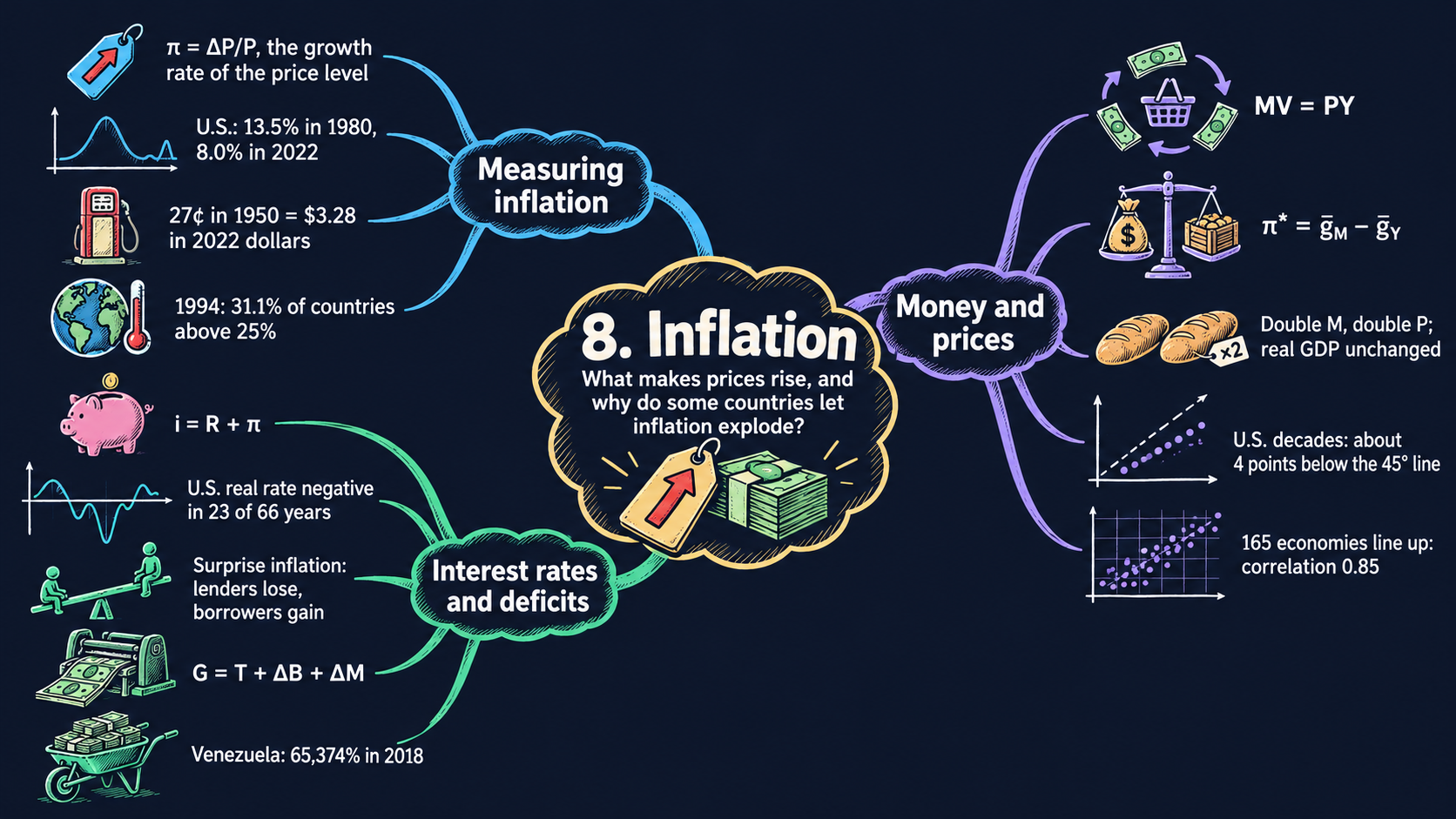
Learning goals

Inflation is the growth rate of the overall price level. By the end of this chapter you will be able to:

measure inflation from a price index, derive average inflation and the rule of 70 from the definition, and convert a price from one year into the dollars of another year with the consumer price index (CPI);
derive the quantity theory of money step by step from its four assumptions, and solve it for the price level, $P^* = \bar{M}\bar{V}/\bar{Y}$, and for inflation, $\pi^* = \bar{g}_M - \bar{g}_Y$;
read the comparative statics of the quantity theory, and explain why money is neutral in the long run (the classical dichotomy);
test the quantity theory with 150 years of U.S. data and with 165 economies;
derive the Fisher equation, $i = R + \pi$, from the return on one saved dollar, and use it to compute real interest rates and to see who gains and who loses from surprise inflation;
derive how much revenue a government raises by printing money (seigniorage), and explain why very high inflation is usually a fiscal problem;
rebuild a price index from inflation rates, compute average growth rates over periods, use ratio scales with clear tick labels, and spot suspicious numbers in a data set.

Model overview

Back on Islandia, the small island country of the earlier chapters, people pay for fish, bread and boat repairs with paper dollars. Only one institution may print those dollars: the Bank of Islandia, the island’s central bank. Year after year the shop prices creep up a little. Why do they rise, and what decides how fast? And why would a government ever let prices run away? This section answers these questions with a few simple models, and we follow Islandia’s dollars through every step.

The big idea

The question. What makes prices rise year after year, how does that change interest rates, and why do some governments let inflation get out of hand?

The answer in one sentence. In the long run prices rise as fast as money grows beyond the growth of the goods it buys: this is the quantity theory of money, and money printed to pay for a deficit is the usual source of very high inflation.

What goes in and what comes out. We choose the money supply and its growth rate, the velocity of money, real GDP and its growth rate, the real interest rate, a tax rate and a budget deficit. The models give back the price level, the inflation rate, the nominal interest rate, the gains and losses of lenders and savers, and the money growth a deficit needs.

Road map.

Measuring inflation: the definitions, and how to work with them: average inflation, doubling times, old prices in today’s dollars.
The quantity theory of money: its four assumptions, the price level and inflation, and neutrality.
The Fisher equation: from the nominal to the real interest rate.
Who gains and who loses from inflation: surprises and taxes on nominal interest.
Seigniorage: the budget constraint, and why very high inflation is fiscal.
Model in code: the key results as Python functions, checked with numbers.

Notation. A bar over a letter marks a parameter: a number we take as given from outside the model, such as $\bar{M}_t$ or $\bar{V}$. Letters without a bar are endogenous variables: the model determines them. In the text rates are in percent; in the algebra they are decimals (2 percent is 0.02).

Symbol	Meaning	Type
$P_t$, $\pi_t$	the price level (an index) and the inflation rate	endogenous
$P^$, $\pi^$	a star marks the price level and inflation that solve the quantity theory	endogenous
$M_t, V_t, Y_t$	money, the velocity of money and real GDP in year $t$	endogenous
$\bar{M}_t, \bar{V}, \bar{Y}_t$	the values of money, velocity and real GDP set outside the model	parameters
$\bar{g}_M, \bar{g}_Y$	the growth rates of money and of real GDP	parameters
$i$, $R$	the nominal and the real interest rate	endogenous
$\pi^e$, $R^e$	expected inflation and the real rate a loan aims for	parameters
$\tau$	the tax rate on interest income	parameter
$G, T, \Delta B, \Delta M$	government spending, taxes, new borrowing and new money	endogenous
$\sigma$	the deficit paid with new money, as a share of GDP	parameter
$g_X$, $\Delta X_{t+1}$	the growth rate $\Delta X_{t+1}/X_t$, and the change $X_{t+1}-X_t$	notation

Islandia’s baseline. Every number below comes from one starting year of Islandia: money $\bar{M} = 100$, velocity $\bar{V} = 2$ and real GDP $\bar{Y} = 200$, money growth $\bar{g}_M = 5$ percent, real GDP growth $\bar{g}_Y = 3$ percent (the starting value of the slider in Fig. 4), and a real interest rate of 2 percent.

Measuring inflation

Definitions

The price level. $P_t$ is the price of a basket of goods in year $t$, written as an index. We pick a base year and set $P = 100$ there. On Islandia, think of the basket as what a typical household buys in a year: fish, bread, rent and a few nets. The consumer price index (CPI) tracks such a household basket; the GDP deflator tracks everything the island produces.

The inflation rate. Inflation is the percentage change of the price level from one year to the next. If Islandia’s index goes from $P_t$ to $P_{t+1}$, the rise is $P_{t+1} - P_t$, and as a share of the old level it is

\[\pi_t = \frac{P_{t+1} - P_t}{P_t}.\]

Key result: the inflation rate

\[\pi_t = \frac{P_{t+1} - P_t}{P_t} \tag{1}\]

A negative $\pi_t$ means that the price level falls: deflation.

Islandia in numbers. If the index moves from 100 to 102, inflation is $2/100 = 2$ percent.

Nominal and real values. A nominal value is counted in the dollars of its own year. A real value is counted in the dollars of one fixed year, so it measures goods, not dollars.

Working with the definitions

From inflation back to the price level. Multiply both sides of equation (1) by $P_t$ and add $P_t$:

\[\pi_t P_t = P_{t+1} - P_t \quad\Longrightarrow\quad P_{t+1} = (1 + \pi_t)P_t.\]

Repeating this step year after year chains the inflation rates together:

\[P_T = P_0(1 + \pi_0)(1 + \pi_1)\cdots(1 + \pi_{T-1}).\]

Fig. 1 builds a price level from inflation rates in exactly this way. With a constant rate $\pi$ the product becomes a power, $P_T = P_0(1+\pi)^T$ (Appendix C.3).

Average inflation over many years. Solve $P_T = P_0(1+\bar{\pi})^T$ for the constant rate $\bar{\pi}$ that connects the first and the last price level. Divide by $P_0$, raise both sides to the power $1/T$, and subtract 1:

\[\left(\frac{P_T}{P_0}\right)^{1/T} = 1 + \bar{\pi} \quad\Longrightarrow\quad \bar{\pi} = \left(\frac{P_T}{P_0}\right)^{1/T} - 1.\]

Fig. 3 uses this formula to measure the average growth of money and prices over decades. Taking logs gives a handy shortcut, $\bar{\pi} \approx (\ln P_T - \ln P_0)/T$ (Appendix C.4).

How long until prices double. Set $P_T/P_0 = 2$ in $P_T = P_0(1+\pi)^T$ and take logs: $T\ln(1+\pi) = \ln 2$. Since $\ln 2 \approx 0.70$ and $\ln(1+\pi) \approx \pi$ for small $\pi$, the doubling time is about $70$ divided by inflation in percent. This is the rule of 70 (Appendix C.3). At 2 percent a year, Islandia’s prices double in about 35 years.

Moving a price from one year to another. A boat that cost $X_a$ dollars in year $a$ took the same share of the basket as $X_a \times P_b/P_a$ dollars in year $b$. The “year-$a$ dollars” cancel, like units in a conversion:

\[X_b = X_a \times \frac{P_b}{P_a}.\]

Key result: converting dollars between years

\[X_b = X_a \times \frac{P_b}{P_a} \tag{2}\]

Only the ratio $P_b/P_a$ matters, so the choice of base year makes no difference (Appendix C.2).

Islandia in numbers. If the index doubles from 100 to 200, a 50-dollar net of the first year is a 100-dollar net of the second.

In words

A price index is a ruler for dollars. Islandia’s dollar shrinks a little every year, so an old price says little until we convert it. Equation (2) turns old dollars into today’s dollars, and only then can we tell whether a boat was cheap or dear.

What it tells us

Small rates add up. At 2 percent a year the price level doubles in 35 years. A dollar of today then buys about half of what a dollar bought 35 years earlier.
Fixed dollar amounts lose value. A pension of 1,000 dollars a year that is never raised buys, after 35 years at 2 percent, what 500 dollars bought at the start: its real value is $1{,}000 \times P_0/P_T$.
An index only compares years. To say whether gasoline was cheap in some past year, turn its old price into today’s dollars with equation (2) before comparing it with today’s price.

Inflation measures how fast prices climb, and a few percent a year doubles them within one working life.

Check your understanding

1. Islandia’s prices rise by 3.5 percent a year. About how long does it take for them to double?

Answer

By the rule of 70, about $70/3.5 = 20$ years. The exact answer, $\ln 2/\ln(1.035)$, is about 20.1 years.

2. A fishing boat cost 400 dollars when Islandia’s price index stood at 80. The index is now 120. What is the boat’s price in today’s dollars, and would a different base year change the answer?

Answer

By equation (2), $400 \times 120/80 = 600$ dollars. A different base year would rescale both index values by the same factor, so their ratio, and the answer, stay the same.

The quantity theory of money

Assumptions

Money is whatever people use to pay for things. On Islandia, think first of the paper notes that the Bank of Islandia prints; Table 8.2 lists broader measures that add bank deposits. Four variables enter the theory, and four equations pin them down.

1. The quantity equation. Each dollar is spent several times a year. The velocity of money $V_t$ counts how many times, on average. So $M_t$ dollars pay for $M_tV_t$ dollars of goods in a year. That spending is nominal GDP: the price level times real GDP.

Key result: the quantity equation

\[M_tV_t = P_tY_t \tag{3}\]

On its own, equation (3) is close to a definition: given $M$, $P$ and $Y$, it measures velocity, $V = PY/M$.

Islandia in numbers. Nominal GDP is $1 \times 200 = 200$ and money is 100, so each Islandian dollar changes hands twice a year.

The equation turns into a theory once we add three more.

2. The classical dichotomy. Real GDP is set by real forces only: Islandia’s tools, its workers, its ideas and their productivity, as in the growth models of Chapters 4 to 6. Money and prices play no part in those models. So for the quantity theory real GDP is given: $Y_t = \bar{Y}_t$.

3. Constant velocity. Payment habits, and the technology people pay with, change slowly. We take velocity as a constant: $V_t = \bar{V}$. It has no time subscript because it does not change over time.

4. The central bank sets the money supply. We do not model how the Bank of Islandia decides; we take its choice as given: $M_t = \bar{M}_t$. (Chapter 12 gives monetary policy a richer model.)

Equation	Name	What it takes as given
$M_tV_t = P_tY_t$	quantity equation	none
$Y_t = \bar{Y}_t$	classical dichotomy	$\bar{Y}_t$, from the growth models
$V_t = \bar{V}$	constant velocity	$\bar{V}$
$M_t = \bar{M}_t$	money supply	$\bar{M}_t$, chosen by the central bank

The endogenous variables are $M_t$, $V_t$, $P_t$ and $Y_t$. Three of the four equations simply set a variable equal to something given from outside.

Solving the model

Step 1: the price level. Put the last three equations into the quantity equation (3):

\[\bar{M}_t\bar{V} = P_t\bar{Y}_t.\]

Only $P_t$ is unknown. Divide both sides by $\bar{Y}_t$:

\[P_t^* = \frac{\bar{M}_t\bar{V}}{\bar{Y}_t}.\]

Key result: the price level

\[P_t^* = \frac{\bar{M}_t\bar{V}}{\bar{Y}_t} \tag{4}\]

The numerator, $\bar{M}_t\bar{V}$, is the spending power of all the money on the island; the denominator is the amount of goods there is to buy. The price level is their ratio.

Islandia in numbers. With $\bar{M} = 100$, $\bar{V} = 2$ and $\bar{Y} = 200$, $P^* = 100 \times 2/200 = 1$.

Step 2: from levels to growth rates. Inflation is the growth rate of $P$, so we turn equation (3) into growth rates. A product grows at the sum of its factors’ growth rates (Appendix C.5). To see where that rule comes from, take logs of equation (3) in two years, $t$ and $t+1$:

\[\ln M_t + \ln V_t = \ln P_t + \ln Y_t, \qquad \ln M_{t+1} + \ln V_{t+1} = \ln P_{t+1} + \ln Y_{t+1}.\]

Subtract the first from the second. Each term becomes a change in a log, $\Delta \ln X = \ln X_{t+1} - \ln X_t$, and the change in a log is approximately the growth rate, $\Delta\ln X \approx g_X$ (Appendix C.4). So money growth plus velocity growth equals inflation plus real GDP growth:

\[\bar{g}_M + \bar{g}_V = g_P + \bar{g}_Y.\]

Step 3: inflation. Velocity is constant, so $\bar{g}_V = 0$. Write $\pi = g_P$ and subtract $\bar{g}_Y$ from both sides:

\[\pi^* = \bar{g}_M - \bar{g}_Y.\]

Key result: the quantity theory of inflation

\[\bar{g}_M + \bar{g}_V = g_P + \bar{g}_Y \tag{5}\]

\[\pi^* = \bar{g}_M - \bar{g}_Y \tag{6}\]

Money that grows as fast as real GDP only keeps up with the extra goods; just the money growth beyond that raises prices.

Islandia in numbers. With $\bar{g}_M = 5$ and $\bar{g}_Y = 3$ percent, inflation is $5 - 3 = 2$ percent. The exact rate below is $1.05/1.03 - 1 \approx 1.94$ percent.

In words

Each year Islandia has 3 percent more fish, bread and boats to sell, and the Bank of Islandia puts 5 percent more dollars into people’s pockets. Three of those five points are soaked up by the extra goods. The other two have nothing new to buy, so they bid up prices.

How exact is the growth-rate rule? In discrete time, write each variable in year $t+1$ as its value in year $t$ times one plus its growth rate, and divide equation (3) for year $t+1$ by equation (3) for year $t$:

\[\frac{M_{t+1}V_{t+1}}{M_tV_t} = \frac{P_{t+1}Y_{t+1}}{P_tY_t} \quad\Longrightarrow\quad (1+\bar{g}_M)(1+\bar{g}_V) = (1+\pi)(1+\bar{g}_Y).\]

With $\bar{g}_V = 0$ the exact inflation rate is

\[\pi = \frac{1+\bar{g}_M}{1+\bar{g}_Y} - 1 = \frac{\bar{g}_M - \bar{g}_Y}{1+\bar{g}_Y}.\]

It differs from equation (6) only by the factor $1/(1+\bar{g}_Y)$, which is close to one. On Islandia the exact rate is $1.05/1.03 - 1 = 1.94$ percent instead of 2 (Appendix C.6).

What the model predicts

Comparative statics. Take logs of equation (4): $\ln P^* = \ln\bar{M} + \ln\bar{V} - \ln\bar{Y}$. Each coefficient is an elasticity, and all of them are one in size. Equation (6) is already linear in growth rates, so its effects are one for one as well.

A change in …	effect on the price level $P^*$	effect on inflation $\pi^*$	what moves in Figs. 3 and 4
money supply $\bar{M}$, up 1% once	$+1\%$	none after that year	nothing
velocity $\bar{V}$, up 1% once	$+1\%$	none after that year	nothing
real GDP $\bar{Y}$, up 1% once	$-1\%$	none after that year	nothing
money growth $\bar{g}_M$, up 1 point	rises faster every year	$+1$ point	the economy moves along the line
real GDP growth $\bar{g}_Y$, up 1 point	rises more slowly	$-1$ point	the line $\pi = g_M - g_Y$ shifts down
velocity growth $\bar{g}_V$ (if not 0), up 1 point	rises faster	$+1$ point	points lie above the line

A one-time change in a level gives a one-time jump in the price level. Only a change in a growth rate changes inflation for good.

Money growth drives inflation. Real GDP growth comes from the slow forces of the growth models and stays in a narrow range, a few percent a year. Money growth is a policy choice and can be anything, from 2 percent to thousands of percent. So large and lasting differences in inflation, over time or across countries, must come from differences in money growth. Figs. 3 and 4 put this prediction to the test.

The neutrality of money. Suppose the Bank of Islandia multiplies the money supply by a factor $\lambda$, say $\lambda = 2$. By equation (4), with $\bar{V}$ and $\bar{Y}$ unchanged, the price level is multiplied by $\lambda$ too. If every price and every wage is multiplied by $\lambda$, every ratio between them stays the same:

\[\frac{\lambda p_{\text{bread}}}{\lambda p_{\text{book}}} = \frac{p_{\text{bread}}}{p_{\text{book}}}, \qquad \frac{\lambda W}{\lambda P} = \frac{W}{P}.\]

Relative prices and the real wage tell islanders what to buy, how much to work and what to produce. None of them changes, so no one has a reason to act differently, and real GDP stays at $\bar{Y}$. A change in the money supply that only changes nominal values is called neutral. The same algebra describes a currency reform that swaps every old note for $\lambda$ new ones. This is why the classical dichotomy describes the long run well.

Only the long run. In the short run, many prices and wages are slow to change. Then more money can move relative prices and real GDP for a while. The short-run model of Chapters 9 to 13 is built on that idea. The quantity theory is a theory of the long run.

In the long run, inflation is money growth minus real growth, and money changes only nominal values.

Check your understanding

1. The Bank of Islandia raises money growth from 5 to 8 percent, while real GDP still grows 3 percent a year. What happens to inflation, by the shortcut and exactly?

Answer

By equation (6), inflation rises from 2 to $8 - 3 = 5$ percent: one point of money growth adds one point of inflation. The exact rate is $1.08/1.03 - 1 \approx 4.85$ percent.

2. The Bank of Islandia swaps every old note for ten new ones, once. What happens to the price level, to inflation in later years, and to the real wage?

Answer

By equation (4) the price level jumps tenfold, once. Money growth after the swap is unchanged, so by equation (6) inflation in later years is unchanged too. Wages and prices are both multiplied by ten, so the real wage $W/P$ stays the same: money is neutral.

Real and nominal interest rates: the Fisher equation

Assumptions

A nominal interest rate $i$ is paid in dollars: put 1 dollar in an Islandian bank today and get $1+i$ dollars back next year. Banks quote nominal rates.
A real interest rate $R$ is paid in goods: give up 1 unit of goods today and get $1+R$ units next year. In the long run it equals the marginal product of capital, the return on one more of Islandia’s tools, as in the Solow model (Chapter 5). So it is set by real forces, just like $\bar{Y}$.
Prices rise at the rate $\pi$ between this year and the next: $P_{t+1} = (1+\pi)P_t$.

Solving the model

Step 1: follow one dollar. With 1 dollar today, an islander can buy $1/P_t$ units of goods. If she saves the dollar instead, she gets $1+i$ dollars next year, which buy $(1+i)/P_{t+1}$ units of goods. Her return in goods is the ratio of the two:

\[1 + R = \frac{(1+i)/P_{t+1}}{1/P_t} = (1+i)\frac{P_t}{P_{t+1}} = \frac{1+i}{1+\pi}.\]

Step 2: solve for the nominal rate. Multiply both sides by $1+\pi$ and expand the product:

\[1 + i = (1+R)(1+\pi) = 1 + R + \pi + R\pi.\]

Step 3: drop the small term. At low rates, $R\pi$ is the product of two small numbers, tiny next to $R$ and $\pi$ themselves (2 percent times 2 percent is only 0.04 percent). Dropping it gives $i = R + \pi$. Subtracting $\pi$ from both sides gives the form we use with data, $R = i - \pi$.

Key result: the Fisher equation

\[i = R + \pi \tag{7}\]

\[R = i - \pi \tag{8}\]

The nominal rate must pay the real return and make up for the shrinking value of the dollars that are repaid. The real rate cannot be looked up: we compute it from a quoted nominal rate and measured inflation, as in Fig. 5.

Islandia in numbers. With $R = 2$ and $\pi = 2$ percent, $i = 4$ percent; the exact formula gives $1.02 \times 1.02 - 1 = 4.04$ percent.

In words

An islander who lends a dollar for a year wants two things back: a real reward for waiting, and compensation for the fish that each dollar will no longer buy. The nominal rate is the sum of the two.

Step 4: the long run. Combine the Fisher equation (7) with the quantity theory (6):

\[i^* = R + \bar{g}_M - \bar{g}_Y.\]

In the long run, $R$ is set by the marginal product of capital and $\bar{g}_Y$ by the growth models. So one more point of money growth raises the nominal interest rate by one point.

What the model predicts

A change in …	nominal rate $i$	real rate $R$
inflation $\pi$ up 1 point, $R$ given (long run)	$+1$ point	unchanged
inflation $\pi$ up 1 point, $i$ fixed in advance	unchanged	$-1$ point
real rate $R$ up 1 point, $\pi$ given	$+1$ point	$+1$ point

High inflation, high nominal rates. Countries and decades with high inflation should have high nominal interest rates, even when their real rates are normal.
Real rates can be negative. If $i$ is below $\pi$, savers lose purchasing power, and equation (8) shows when that happens. A negative real rate could not last in the long run, because the marginal product of capital is positive. When we see one in the data, it tells us that the short run differs from the long run.
The shortcut fails at high inflation. The exact rate is $R = (1+i)/(1+\pi) - 1$. With 14 percent nominal and 72 percent inflation, equation (8) gives $-58$ percent but the exact formula gives $-34$ percent (Appendix C.6).

The nominal interest rate is the real rate plus inflation, so lasting inflation means high nominal rates.

Check your understanding

1. An Islandian bank pays 6 percent on deposits, and inflation is 4 percent. What real return does a saver earn, by the shortcut and exactly?

Answer

By equation (8), $R = 6 - 4 = 2$ percent. The exact rate is $1.06/1.04 - 1 \approx 1.92$ percent, very close because both rates are low.

2. The Bank of Islandia raises money growth by one point for good. In the long run, what happens to the nominal and to the real interest rate?

Answer

By equation (6) inflation rises by one point. The real rate is set by the marginal product of capital, so it does not move, and by equation (7) the nominal rate rises by one point: $i^* = R + \bar{g}_M - \bar{g}_Y$.

Who gains and who loses from inflation

The book discusses the costs of inflation in words. The Fisher equation turns two of them into numbers.

Assumptions

Harbor Boatworks, Islandia’s boatyard, borrows from islanders to pay for a new workshop. Lender and borrower agree on a nominal rate $i$ for some years. They set it with the inflation they expect, $\pi^e$, so that $i = R^e + \pi^e$, where $R^e$ is the real rate both of them want.
The Islandia Treasury taxes interest income at the rate $\tau$ on its nominal amount, as most tax systems do.

Solving the model

A surprise. Once the rate is fixed, the real rate the lenders actually earn comes from equation (8) with the inflation that actually happens:

\[R = i - \pi = (R^e + \pi^e) - \pi = R^e - (\pi - \pi^e).\]

Every point of unexpected inflation, $\pi - \pi^e$, takes one point of real return from the lender and hands it to the borrower.

Taxes on nominal interest. Now let inflation be expected, so that $i = R + \pi$, but let the tax apply to all of $i$. The saver keeps $(1-\tau)i$ dollars of interest, and inflation still takes $\pi$, so her real return after tax is

\[(1-\tau)i - \pi = (1-\tau)(R + \pi) - \pi = (1-\tau)R - \tau\pi.\]

The last step multiplies out $(1-\tau)\pi - \pi = -\tau\pi$. So the tax also falls on the part of the interest that only makes up for inflation. As a share of the real return $R$, the tax actually paid is $\tau R + \tau\pi$: an effective tax rate of $\tau(1 + \pi/R)$.

Key result: winners and losers

\[R = R^e - (\pi - \pi^e) \qquad\text{and}\qquad (1-\tau)i - \pi = (1-\tau)R - \tau\pi\]

The first formula prices a surprise; the second shows the tax on the inflation part of interest. The effective tax rate on the real return is $\tau(1 + \pi/R)$.

Islandia in numbers. The workshop loan is set at $i = 2 + 2 = 4$ percent. If inflation turns out to be 8 percent, the lenders earn $4 - 8 = -4$ percent in real terms. With $\tau = 25$ percent and $R = 2$ percent, the effective tax rate is $0.25 \times (1 + 2/2) = 50$ percent at 2 percent inflation, and $0.25 \times (1 + 8/2) = 125$ percent at 8 percent inflation, when the after-tax real return turns negative.

In words

When prices jump unexpectedly, Harbor Boatworks repays its loan with dollars that buy fewer fish than everyone planned. The boatyard gains what its lenders lose. And even fully expected inflation hurts savers when the Treasury taxes the part of interest that only keeps up with prices.

What the model predicts

Surprises redistribute. Unexpected inflation moves wealth from lenders, savers and people on fixed nominal incomes to borrowers. Unexpected disinflation does the opposite. Expected inflation that is built into contracts does neither.
Inflation raises taxes on saving. When taxes fall on nominal returns, higher inflation lowers the after-tax real return even when it is fully expected. That discourages saving and investment.
Indexing removes both effects. Contracts, pensions and taxes written in real terms (adjusted for $\pi$) would make steady, known inflation little more than a nuisance. The real cost of inflation comes from surprises, and from rules written in dollars.

Surprise inflation shifts wealth from lenders to borrowers; taxes on nominal interest make even expected inflation costly for savers.

Check your understanding

1. The workshop loan was set at 4 percent when everyone expected 2 percent inflation, but inflation turns out to be only 1 percent. What real return do the lenders earn? Who gains?

Answer

By the surprise formula, $R = 2 - (1 - 2) = 3$ percent, or simply $4 - 1 = 3$ percent by equation (8). The lenders gain one point and Harbor Boatworks loses it: an unexpected disinflation redistributes toward lenders.

2. With $\tau = 25$ percent, $R = 2$ percent and expected inflation of 4 percent, what is a saver’s after-tax real return, and what is the effective tax rate?

Answer

The after-tax real return is $(1-\tau)R - \tau\pi = 0.75 \times 2 - 0.25 \times 4 = 0.5$ percent. The effective tax rate is $\tau(1 + \pi/R) = 0.25 \times 3 = 75$ percent of the real return, three times the legal rate.

Seigniorage and the fiscal causes of high inflation

Assumptions

The Islandia Treasury spends $G$ dollars a year. It pays with taxes $T$, with new borrowing $\Delta B$ (the change in its debt $B$), or with new money $\Delta M$ (the change in the money stock $M$), which the Bank of Islandia prints for it.
The money in this block is the money the state itself issues: currency, or the monetary base. Its velocity $\bar{V}$ is nominal GDP divided by currency. We give Islandia $\bar{V} = 12$, close to the U.S. value in 2023.
The quantity theory holds, with constant velocity.

Solving the model

Step 1: the budget constraint. Uses of funds equal sources of funds: $G = T + \Delta B + \Delta M$. Solved for the new money, $\Delta M = G - T - \Delta B$: whatever spending is not covered by taxes or new loans must be covered by printing money. The revenue from new money is called seigniorage, or the inflation tax.

Step 2: seigniorage as a share of GDP. Divide the new money by nominal GDP and write $\Delta M_t = \bar{g}_M M_{t-1}$, where $M_{t-1}$ is last year’s stock. Since $M_t = (1+\bar{g}_M)M_{t-1}$ and, by the quantity equation (3), $M_t = P_tY_t/\bar{V}$,

\[\frac{\Delta M_t}{P_tY_t} = \frac{\bar{g}_M M_{t-1}}{P_tY_t} = \frac{\bar{g}_M}{1+\bar{g}_M}\cdot\frac{M_t}{P_tY_t} = \frac{\bar{g}_M}{(1+\bar{g}_M)\bar{V}}.\]

For low rates $1+\bar{g}_M \approx 1$, and the quantity theory (6) gives $\bar{g}_M = \pi^* + \bar{g}_Y$.

Key result: the budget constraint and seigniorage

\[G = T + \Delta B + \Delta M \tag{9}\]

\[\frac{\Delta M_t}{P_tY_t} = \frac{\bar{g}_M}{(1+\bar{g}_M)\bar{V}} \approx \frac{\pi^* + \bar{g}_Y}{\bar{V}} \tag{10}\]

Islandia in numbers. With 2 percent inflation, 3 percent real growth and $\bar{V} = 12$, new money pays for about $5/12 \approx 0.4$ percent of GDP a year.

Step 3: who pays. Split equation (10) into two parts. The part $\bar{g}_Y/\bar{V}$ is new money that islanders want anyway, because a growing economy needs more money for its payments; it causes no inflation. The part $\pi^*/\bar{V}$ is a tax. Every dollar people hold loses the share $\pi/(1+\pi)$ of its purchasing power each year, so the tax rate is about $\pi$, and the tax base is the real money people hold. Holders of currency pay it. Owners of land, houses or shares do not, because those prices rise with all the others.

In words: the inflation tax

Every new dollar the Bank of Islandia prints for the Treasury buys real fish and real boats. Nobody sends a tax bill, yet someone pays: every islander holding notes finds that they buy a little less each year.

Step 4: how much inflation a deficit needs. Suppose lenders stop lending, $\Delta B = 0$, and taxes fall short of spending by a share $\sigma$ of GDP. Then equation (10) must equal $\sigma$. Multiply both sides by $(1+\bar{g}_M)\bar{V}$, collect the terms in $\bar{g}_M$, and solve (Appendix C.9):

\[\sigma\bar{V}(1+\bar{g}_M) = \bar{g}_M \quad\Longrightarrow\quad \sigma\bar{V} = \bar{g}_M(1 - \sigma\bar{V}) \quad\Longrightarrow\quad \bar{g}_M = \frac{\sigma\bar{V}}{1-\sigma\bar{V}}.\]

Inflation then follows from the exact quantity theory, $\pi = (1+\bar{g}_M)/(1+\bar{g}_Y) - 1$. A deficit of 5 percent of GDP with $\bar{V} = 12$ gives $\sigma\bar{V} = 0.6$, money growth of $0.6/0.4 = 150$ percent, and inflation of about 143 percent a year.

What the model predicts

Persistent high inflation is fiscal. Rich countries raise well under 1 percent of GDP with new money, because inflation is low and people hold little currency. A government that loses access to taxes and loans must print money, and the quantity theory turns that money into inflation.
The printing press has a ceiling. Since $\bar{g}_M/(1+\bar{g}_M) < 1$, seigniorage stays below $1/\bar{V}$ of GDP however fast money grows: about 8 percent of GDP with $\bar{V} = 12$. In practice the ceiling is lower, because people hold less money when it loses value fast, so velocity rises. A deficit close to the ceiling needs explosive money growth: this is the arithmetic of hyperinflation.
Ending a hyperinflation needs a fiscal fix. Inflation falls when money growth falls, and by equation (9) money growth can fall only when spending falls, taxes rise or borrowing resumes. An independent central bank, one that the treasury cannot order to print, is a way to close the third option before a crisis.

Very high inflation starts in the budget: a government that cannot tax or borrow prints money, and prices follow.

Check your understanding

1. Lenders refuse to lend to the Islandia Treasury, and it must pay for a deficit of 2 percent of GDP with new money. With $\bar{V} = 12$ and real growth of 3 percent, what money growth and inflation does this take?

Answer

By step 4, $\sigma\bar{V} = 0.02 \times 12 = 0.24$, so $\bar{g}_M = 0.24/0.76 \approx 31.6$ percent. The exact quantity theory gives $\pi = 1.316/1.03 - 1 \approx 27.7$ percent a year.

2. Could the Treasury pay for a deficit of 10 percent of GDP with new money alone?

Answer

No. By equation (10), seigniorage stays below $1/\bar{V} = 1/12 \approx 8.3$ percent of GDP however fast money grows. In step 4, $\sigma\bar{V} = 1.2$ is above one, so no money growth solves the equation. Only lower spending, higher taxes or new loans can close that gap.

Recap

Inflation is how fast the price level climbs, and small rates compound: at 2 percent prices double in about 35 years (Fig. 1).
The quantity theory gives $P^* = \bar{M}\bar{V}/\bar{Y}$ and $\pi^* = \bar{g}_M - \bar{g}_Y$: lasting inflation comes from money growth (Fig. 3 and Fig. 4).
Money is neutral in the long run: scaling all money scales all prices and leaves real GDP and the real wage alone.
The Fisher equation $i = R + \pi$ links inflation to nominal rates, and $R = i - \pi$ measures real rates, as Fig. 5 does with data.
Surprises and nominal taxes move wealth from lenders and savers to borrowers and the state.
Very high inflation is fiscal: a deficit paid with new money needs fast money growth, and seigniorage has a ceiling of $1/\bar{V}$ (Fig. 6).

Model in code

Now we turn the Key results into Python. The section has four parts: the setup (folded, because it is the same in every chapter), the model as functions, numerical checks of the Key results, and the data tools that give every country its color in the figures (folded too). Run its cells once, in order. Every later section of the notebook reuses them.

Setup

Run the setup cells once, before anything else. They load the Python libraries, give every chart the same look, store the address of the chapter’s data and define three helpers that only the book website needs. You can use the notebook without reading them; open the box if you are curious.

Show the setup code

The first cell loads the libraries and sets the look of the charts. Its comments explain each step.

# @title Setup: libraries, chart colors and the data location
# Text after a "#" is a comment: Python ignores it, it is there for human readers.

# Step 1: load the libraries. `import` loads a library, a toolbox written by
# other people, and `as pd` gives it a short nickname, so the code stays short.
import numpy as np                    # numbers and arrays
import pandas as pd                   # data tables
import plotly.express as px           # quick charts from data tables
import plotly.graph_objects as go     # charts built piece by piece
import plotly.io as pio               # settings shared by every chart
# sliders, buttons and lists for the interactive figures
from ipywidgets import interact, FloatSlider, ToggleButtons, Dropdown, SelectMultiple

# Step 2: one light blue/green look for every chart
BLUE, TEAL, GREEN, GRAY = "#16528c", "#008070", "#7fb23a", "#8a96a3"
ORANGE = "#e0a33b"                    # a fourth color for the country comparisons
pio.templates.default = "plotly_white"
# the same chart size in Colab and on the website
pio.templates["plotly_white"].layout.update(width=860, height=480)
px.defaults.color_discrete_sequence = [BLUE, TEAL, GREEN, "#5aa0d8", "#0b4f47"]
WIDE = {"description_width": "initial"}         # show the full slider labels

# Step 3, Colab only: let Plotly charts appear inside the interactive widgets.
# `try` runs the indented lines; if the import fails (we are not in Colab),
# `except` skips them.
try:
    import google.colab
    google.colab.output.enable_custom_widget_manager()
except ImportError:
    pass                                        # not running in Colab: nothing to do

# Step 4: the data files of this chapter live in the book's GitHub repository
DATA_URL = "https://raw.githubusercontent.com/quarcs-lab/macro102-site/main/data/ch08/"

The website cannot run Python, so each interactive figure also gets a version with a precomputed slider. The next helper builds those versions. Run it and move on.

# @title Helper for the website versions (run this cell; you do not need to read it)
def slider_figure(make_figure, name, values, start, label=None):
    """Join precomputed versions of a figure with one slider (the website cannot run Python).

    Arguments
        make_figure : the function that draws the figure
        name        : the argument the slider moves
        values      : the values of that argument to precompute
        start       : the value shown first
        label       : the slider's label (the argument name if None)
    Returns
        one Plotly figure with all versions and a slider that shows one at a time
    """
    # Step 1: draw the figure once for every value
    figures = [make_figure(**{name: v}) for v in values]
    first = values.index(start)
    # Step 2: copy every curve into one figure; only the start value's are visible
    fig = go.Figure(layout=figures[first].layout)
    owner = []                                  # which figure each trace comes from
    for i, f in enumerate(figures):
        for trace in f.data:
            trace.visible = (i == first)
            fig.add_trace(trace)
            owner.append(i)
    # Step 3: one slider step per value: its curves, title, labels and shapes
    steps = []
    for i, f in enumerate(figures):
        layout = {"title": f.layout.title.to_plotly_json(),
                  "annotations": [a.to_plotly_json() for a in f.layout.annotations],
                  "shapes": [s.to_plotly_json() for s in f.layout.shapes]}
        visible = [o == i for o in owner]
        steps.append(dict(method="update", label=str(values[i]), args=[{"visible": visible}, layout]))
    fig.update_layout(sliders=[dict(active=first, steps=steps, pad=dict(t=60),
                                    currentvalue=dict(prefix=(label or name) + " = "))])
    return fig

The data figures show many countries. On the website, the next two helpers draw the textbook’s countries, keep every other country one click away in the legend, and add buttons for a linear or a ratio scale.

# @title Helpers for the website's country legends (run this cell; you do not need to read it)
def legend_only(fig, keep):
    """Start every trace not named in `keep` hidden, but in the legend: one click shows it.

    Slider steps keep the choice, so a slider never switches on all countries at once.

    Arguments
        fig  : a Plotly figure with one trace per country (and perhaps a slider)
        keep : the names of the traces drawn at the start
    Returns
        the same figure, with the visibility set in the figure and in every slider step
    """
    # Step 1: hide every trace that is not kept, but leave it in the legend
    names = [t.name for t in fig.data]
    for t in fig.data:
        if t.visible is not False and t.name not in keep:
            t.visible = "legendonly"
    # Step 2: make every slider step keep the same choice
    for slider in fig.layout.sliders:
        steps = []
        for step in slider.steps:
            # a trace the step hides stays hidden; one it shows is drawn only if kept
            shown = []
            for name, v in zip(names, step.args[0]["visible"]):
                shown.append(v if (v is False or name in keep) else "legendonly")
            steps.append(dict(method=step.method, label=step.label, args=[{"visible": shown}, step.args[1]]))
        # replace the old steps by the new ones
        slider.steps = steps
    return fig


def scale_buttons(fig, ratio_ticks, start="linear"):
    """Add buttons that switch the vertical axis between a linear and a ratio scale.

    The axis then fits whatever countries are shown.

    Arguments
        fig         : the figure to add the buttons to
        ratio_ticks : the tick values of the ratio (log) scale
        start       : the scale shown first, "linear" or "ratio"
    Returns
        the same figure, with the two buttons
    """
    # Step 1: the two buttons; each sets the axis type and refits the axis
    linear = dict(label="linear scale", method="relayout",
                  args=[{"yaxis.type": "linear", "yaxis.autorange": True, "yaxis.tickvals": None}])
    ratio = dict(label="ratio scale", method="relayout",
                 args=[{"yaxis.type": "log", "yaxis.autorange": True, "yaxis.tickvals": ratio_ticks}])
    # Step 2: the starting scale comes first, then the buttons go in the top left corner
    buttons = [linear, ratio] if start == "linear" else [ratio, linear]
    fig.update_layout(updatemenus=[dict(type="buttons", direction="right", x=0.01, y=0.98, xanchor="left",
                                        yanchor="top", buttons=buttons)])
    fig.update_yaxes(autorange=True)
    return fig

The model as functions

The Key results of this chapter are short formulas: the price level of the quantity theory, equation (4), inflation in growth rates, equations (5) and (6), and the Fisher equation in its two forms, equations (7) and (8). We write each one as a Python function: a named recipe that takes inputs and gives back a result. All rates here are in percent. The first two functions are the quantity theory.

# `def` creates a function. Its inputs are the arguments in parentheses.
# The text in triple quotes describes the function.
def price_level(M, V, Y):
    """The price level that solves the quantity equation M V = P Y.

    Equation (4):  P* = M V / Y

    Arguments
        M : the money supply, M-bar
        V : the velocity of money, V-bar
        Y : real GDP, Y-bar
    Returns
        the price level, P*
    """
    # `return` gives back the result: the quantity equation solved for P
    return M * V / Y


# `g_V=0.0` gives g_V a default value, used whenever we do not pass one:
# velocity is constant unless we say otherwise
def qt_inflation(g_M, g_Y, g_V=0.0):
    """Inflation from the quantity theory, in growth rates (percent).

    Equations (5) and (6):  pi* = g_M + g_V - g_Y, and pi* = g_M - g_Y when g_V = 0

    Arguments
        g_M : the growth rate of money, g-bar_M (percent)
        g_Y : the growth rate of real GDP, g-bar_Y (percent)
        g_V : the growth rate of velocity (percent; 0 when velocity is constant)
    Returns
        the inflation rate, pi* (percent)
    """
    # money growth beyond the growth of the goods it buys becomes inflation
    return g_M + g_V - g_Y

The Fisher equation links the nominal interest rate $i$, the real interest rate $R$ and inflation $\pi$. Equation (7) gives the nominal rate, and equation (8), the same equation solved for $R$, gives the real rate.

def nominal_rate(R, pi):
    """The nominal interest rate, from the Fisher equation (percent).

    Equation (7):  i = R + pi

    Arguments
        R  : the real interest rate (percent)
        pi : the inflation rate (percent)
    Returns
        the nominal interest rate, i (percent)
    """
    # lenders ask for the real return plus compensation for inflation
    return R + pi


def real_rate(i, pi):
    """The real interest rate, from the Fisher equation (percent).

    Equation (8):  R = i - pi

    Arguments
        i  : the nominal interest rate (percent)
        pi : the inflation rate (percent)
    Returns
        the real interest rate, R (percent)
    """
    # the nominal return minus what inflation takes away
    return i - pi

The last function makes the quantity theory move through time. Money and real GDP grow year by year, and in every year equation (4) gives the price level. A table with one row per year holds the path.

def simulate_prices(g_M=5.0, g_Y=3.0, V=2.0, years=5):
    """Money, real GDP and the price level year by year, with constant growth rates.

    Equation (4) in every year:  P_t = M_t V / Y_t, and inflation is the growth rate of P_t

    Arguments
        g_M   : the growth rate of money, g-bar_M (percent)
        g_Y   : the growth rate of real GDP, g-bar_Y (percent)
        V     : the velocity of money, V-bar
        years : the number of years after the starting year
    Returns
        a table with the columns year, M, Y, P and inflation (percent)
    """
    # Step 1: Islandia's starting year
    M, Y = 100.0, 200.0
    # Step 2: one row per year. `rows.append([...])` adds one row to the list,
    # then money and real GDP grow for the next year
    rows = []
    for t in range(years + 1):
        rows.append([t, M, Y, price_level(M, V, Y)])
        M = M * (1 + g_M / 100)
        Y = Y * (1 + g_Y / 100)
    # Step 3: `pd.DataFrame(rows, columns=[...])` turns the list into a table;
    # `.pct_change()` is the change from the previous row, as a fraction
    path = pd.DataFrame(rows, columns=["year", "M", "Y", "P"])
    path["inflation"] = 100 * path.P.pct_change()
    return path

Checking the key results

The formulas came from algebra. Now we check them with numbers, one Key result at a time, using Islandia’s baseline: $\bar{M} = 100$, $\bar{V} = 2$, $\bar{Y} = 200$, money growth of 5 percent and real GDP growth of 3 percent.

Check 1: measuring inflation. Start a price index at 100 and let it grow by 2 percent a year for 35 years, using $P_{t+1} = (1+\pi)P_t$ from equation (1). The rule of 70 says it should about double. Then we recover the average rate from the two ends, and use equation (2) to convert a price and a fixed pension.

# Step 1: 35 years of 2% inflation. `range(35)` counts 0, 1, ..., 34, so the `for`
# loop runs its indented line 35 times; `P = P * 1.02` replaces the old P by the new
P = 100.0
for year in range(35):
    P = P * 1.02                                  # one more year of 2% inflation
# Step 2: the price level and the rule of 70. An f-string, f"... {P:.1f}", puts
# a value into the text; ":.1f" means "one decimal"
print(f"Price level after 35 years at 2%: {P:.1f}  (rule of 70: doubling in 70 / 2 = {70 / 2:.0f} years)")
# Step 3: average inflation from the two ends, exactly and with logs
# (`np.log` is the natural logarithm)
print(f"Average inflation from the two ends: {100 * ((P / 100) ** (1 / 35) - 1):.3f}%")
print(f"Log shortcut, (ln P_T - ln P_0) / T:  {100 * (np.log(P) - np.log(100)) / 35:.3f}%")
# Step 4: equation (2), a price and a fixed pension in the dollars of another year
print(f"A 50-dollar item at P = 100 costs {50 * 200 / 100:.0f} dollars at P = 200   (equation 2)")
print(f"A fixed pension of 1,000 dollars buys what {1000 * 100 / P:.0f} dollars bought 35 years earlier")

Price level after 35 years at 2%: 200.0  (rule of 70: doubling in 70 / 2 = 35 years)
Average inflation from the two ends: 2.000%
Log shortcut, (ln P_T - ln P_0) / T:  1.980%
A 50-dollar item at P = 100 costs 100 dollars at P = 200   (equation 2)
A fixed pension of 1,000 dollars buys what 500 dollars bought 35 years earlier

The log shortcut is slightly below 2 percent, because $\ln(1.02) = 0.0198$.

Check 2: the price level and neutrality. Equation (4) with our baseline should give $P^* = 1$. Raising $\bar{M}$, $\bar{V}$ or $\bar{Y}$ by 1 percent should move $P^*$ by $+1$, $+1$ and $-1$ percent. And doubling money should double every nominal value but leave the real wage alone.

# Step 1: the baseline price level, and with money doubled (equation 4)
P_base = price_level(M=100, V=2, Y=200)
print(f"Baseline: P* = {P_base:.2f};  money doubled to 200: P* = {price_level(200, 2, 200):.2f}")
# Step 2: P* with one parameter 1% higher, relative to the baseline
change_M = price_level(100 * 1.01, 2, 200) / P_base - 1
change_V = price_level(100, 2 * 1.01, 200) / P_base - 1
change_Y = price_level(100, 2, 200 * 1.01) / P_base - 1
# ":+.3f" also shows the sign
print(f"1% more money:    P* changes by {100 * change_M:+.3f}%")
print(f"1% more velocity: P* changes by {100 * change_V:+.3f}%")
print(f"1% more real GDP: P* changes by {100 * change_Y:+.3f}%")
# Step 3: neutrality: doubling money doubles the wage and the price of bread
wage, bread = 30.0, 3.0                           # dollars per hour, dollars per loaf
print(f"Real wage before: {wage / bread:.0f} loaves an hour;  after doubling: {2 * wage / (2 * bread):.0f} loaves an hour")

Baseline: P* = 1.00;  money doubled to 200: P* = 2.00
1% more money:    P* changes by +1.000%
1% more velocity: P* changes by +1.000%
1% more real GDP: P* changes by -0.990%
Real wage before: 10 loaves an hour;  after doubling: 10 loaves an hour

The effect of real GDP is $-0.990$ rather than exactly $-1$ percent, because $1/1.01 = 0.990$: an elasticity describes very small changes.

Check 3: the growth-rate version. We let money and real GDP grow year by year and solve equation (4) in every year. Inflation should be the exact rate $1.05/1.03 - 1$, close to the shortcut of equation (6). First the path itself, with the baseline growth rates:

# five years of 5% money growth and 3% real GDP growth, rounded to three decimals
simulate_prices().round(3)

	year	M	Y	P	inflation
0	0	100.000	200.000	1.000	NaN
1	1	105.000	206.000	1.019	1.942
2	2	110.250	212.180	1.039	1.942
3	3	115.762	218.545	1.059	1.942
4	4	121.551	225.102	1.080	1.942
5	5	127.628	231.855	1.101	1.942

Then the same path with faster money growth, compared with the exact rate and with equation (6).

# Step 1: for each rate of money growth, the inflation of the last simulated year
# (`.iloc[-1]` picks the last row), the exact rate and the shortcut of equation (6)
for g_M in (5, 6, 100):
    simulated = simulate_prices(g_M=g_M).inflation.iloc[-1]
    exact = 100 * ((1 + g_M / 100) / 1.03 - 1)
    print(f"Money growth {g_M:3d}%: simulated {simulated:7.3f}%, exact {exact:7.3f}%, equation (6) {qt_inflation(g_M, 3):5.1f}%")
# Step 2: equation (5), with velocity falling 1% a year
print(f"Velocity falling 1% a year, equation (5): inflation {qt_inflation(5, 3, g_V=-1):.1f}%")

Money growth   5%: simulated   1.942%, exact   1.942%, equation (6)   2.0%
Money growth   6%: simulated   2.913%, exact   2.913%, equation (6)   3.0%
Money growth 100%: simulated  94.175%, exact  94.175%, equation (6)  97.0%
Velocity falling 1% a year, equation (5): inflation 1.0%

Inflation is 1.942 percent in every year, not exactly 2, and one more point of money growth adds about one point of inflation. For the moderate rates of Figs. 1 to 5 the shortcut is very close. For the hyperinflations of Figs. 6 and 7 it is not (94 percent instead of 97 here), but the message is the same: more money growth, more inflation.

Check 4: the Fisher equation. Follow one dollar as in step 1, and compare the shortcut of equations (7) and (8) with the exact formula, at low and at very high inflation.

# Step 1: one saved dollar's return in goods, exactly
goods_today = 100 / 1.00                          # 100 dollars at P = 1
goods_next_year = 100 * 1.04 / 1.02               # 104 dollars at P = 1.02
print(f"Exact real return on a 4% deposit with 2% inflation: {100 * (goods_next_year / goods_today - 1):.2f}%")
# Step 2: equation (7) against the exact (1 + R)(1 + pi) - 1
print(f"Equation (7), R = 2%, pi = 2%: i = {nominal_rate(2, 2):.1f}%;  exact (1+R)(1+pi) - 1 = {100 * (1.02 * 1.02 - 1):.2f}%")
# Step 3: equation (8) at low and at very high inflation. The loop walks through
# pairs: first i = 4 and pi = 2, then i = 14 and pi = 72
for i, pi in ((4, 2), (14, 72)):
    exact = 100 * ((1 + i / 100) / (1 + pi / 100) - 1)
    print(f"i = {i}%, pi = {pi}%: R = {real_rate(i, pi):+.2f}% by equation (8), {exact:+.2f}% exact")
# Step 4: the long run, equation (7) with the inflation of equation (6)
print(f"Long run, R = 2%: i* = {nominal_rate(2, qt_inflation(5, 3)):.0f}% with 5% money growth, "
      f"{nominal_rate(2, qt_inflation(6, 3)):.0f}% with 6%")

Exact real return on a 4% deposit with 2% inflation: 1.96%
Equation (7), R = 2%, pi = 2%: i = 4.0%;  exact (1+R)(1+pi) - 1 = 4.04%
i = 4%, pi = 2%: R = +2.00% by equation (8), +1.96% exact
i = 14%, pi = 72%: R = -58.00% by equation (8), -33.72% exact
Long run, R = 2%: i* = 4% with 5% money growth, 5% with 6%

Check 5: surprises and taxes. A loan fixed at 4 percent loses its real value when inflation jumps. With a 25 percent tax on nominal interest, the after-tax real return computed directly must equal $(1-\tau)R - \tau\pi$.

# Step 1: a surprise. The loan's rate is fixed before inflation is known
# the rate is set when everyone expects 2% inflation
contract = nominal_rate(R=2, pi=2)
for pi in (2, 8):
    print(f"Loan at {contract:.0f}%, inflation turns out {pi}%: real return {real_rate(contract, pi):+.1f}%")
# Step 2: a 25% tax on nominal interest, with inflation expected
tau, R = 0.25, 2
for pi in (2, 8):
    # expected inflation: i moves one for one with pi
    i = nominal_rate(R, pi)
    # tax on all of i, then subtract inflation; the formula must give the same
    after_tax = (1 - tau) * i - pi
    formula = (1 - tau) * R - tau * pi
    print(f"pi = {pi}%: i = {i}%, after-tax real return {after_tax:+.2f}% (formula {formula:+.2f}%), "
          f"effective tax rate {100 * (R - after_tax) / R:.0f}%")

Loan at 4%, inflation turns out 2%: real return +2.0%
Loan at 4%, inflation turns out 8%: real return -4.0%
pi = 2%: i = 4%, after-tax real return +1.00% (formula +1.00%), effective tax rate 50%
pi = 8%: i = 10%, after-tax real return -0.50% (formula -0.50%), effective tax rate 125%

Check 6: seigniorage. One year of our economy, now with currency as the money and $\bar{V} = 12$. The new money as a share of GDP must match the exact formula in equation (10), and the shortcut should be close.

# Step 1: one year of Islandia with currency as the money
V_cash = 12                                       # nominal GDP / currency
# currency and real GDP: P = 100 x 12 / 1200 = 1
M, Y = 100.0, 1200.0
# one year of 5% money growth and 3% real growth
M_next, Y_next = M * 1.05, Y * 1.03
P_next = price_level(M_next, V_cash, Y_next)
# Step 2: the new money as a share of GDP: directly, by equation (10), and its shortcut
direct = 100 * (M_next - M) / (P_next * Y_next)
exact = 100 * 0.05 / (1.05 * V_cash)
shortcut = (qt_inflation(5, 3) + 3) / V_cash
print(f"Price level next year: {P_next:.4f} (inflation {100 * (P_next - 1):.2f}%)")
print(f"New money: {direct:.3f}% of GDP directly, {exact:.3f}% exact, {shortcut:.3f}% by the shortcut")

Price level next year: 1.0194 (inflation 1.94%)
New money: 0.397% of GDP directly, 0.397% exact, 0.417% by the shortcut

Check 7: financing a deficit with money. Step 4 solved for the money growth that pays for a deficit of 5 percent of GDP. Putting that money growth back into equation (10) must return 5 percent. The last lines show the ceiling $1/\bar{V}$.

# Step 1: the money growth that pays for the deficit (step 4), and its inflation
# the deficit to be paid with new money, as a share of GDP
sigma = 0.05
g_M = sigma * V_cash / (1 - sigma * V_cash)
pi = (1 + g_M) / 1.03 - 1
print(f"Money growth needed: {100 * g_M:.0f}%;  inflation: {100 * pi:.0f}%")
print(f"Check, equation (10): new money = {100 * g_M / ((1 + g_M) * V_cash):.2f}% of GDP")
# Step 2: seigniorage at ever faster money growth, and the ceiling 1 / V
# money growth of 100%, 1,000% and 10,000% a year
for growth_rate in (1.0, 10.0, 100.0):
    share = 100 * growth_rate / ((1 + growth_rate) * V_cash)
    print(f"Money growth {100 * growth_rate:7,.0f}%: seigniorage {share:.2f}% of GDP")
print(f"Ceiling 1 / V: {100 / V_cash:.2f}% of GDP")

Money growth needed: 150%;  inflation: 143%
Check, equation (10): new money = 5.00% of GDP
Money growth     100%: seigniorage 4.17% of GDP
Money growth   1,000%: seigniorage 7.58% of GDP
Money growth  10,000%: seigniorage 8.25% of GDP
Ceiling 1 / V: 8.33% of GDP

Even 10,000 percent money growth raises less than the ceiling of 8.33 percent of GDP, and only if velocity stayed at 12. In a real hyperinflation people flee from money, velocity rises, and the ceiling falls.

Drawing and data tools

The textbook’s figures show the United States and a few other countries, and every data figure of this notebook lets you add more. The tools here load the list of countries and give each one a color that it keeps from chart to chart. Run them and move on, or open the box to see how they work.

Show the drawing and data tools

A small file lists the World Bank’s 217 economies, with their region, income group and OECD membership:

# @title Data tool: the list of countries
# read the file into a table and show its first five rows
countries = pd.read_csv(DATA_URL + "countries.csv")
countries.head()

	iso3	country	region	income	oecd
0	AFG	Afghanistan	Middle East & North Africa	Low income	False
1	ALB	Albania	Europe & Central Asia	Upper middle income	False
2	DZA	Algeria	Middle East & North Africa	Upper middle income	False
3	ASM	American Samoa	East Asia & Pacific	High income	False
4	AND	Andorra	Europe & Central Asia	High income	False

So that a country keeps its color from chart to chart, and two countries shown together never share one, we give the colors with a small tool. Its palette has 44 colors: Plotly’s 24 dark ones, and the 20 darker ones of its 26 “Alphabet” colors.

# @title Drawing tool: the palette of 44 country colors
# Step 1: `PALETTE = []` starts an empty list, and `.append` adds one color at a time
# the colors too pale on white
LIGHT = ["#F7E1A0", "#E2E2E2", "#FBE426", "#16FF32", "#1CFFCE", "#2ED9FF"]
PALETTE = []
# Plotly's 24 dark colors, all but one medium blue
for c in px.colors.qualitative.Dark24:
    if c != "#2E91E5":
        PALETTE.append(c)
# Step 2: the 20 Alphabet colors that are not too pale: 44 in all
for c in px.colors.qualitative.Alphabet:
    if c not in LIGHT:
        PALETTE.append(c)
# Step 3: the medium blue, too close to the U.S. navy, is used last
PALETTE.append("#2E91E5")

first_free picks one color: the first one nobody uses yet, or, when every color is taken, the one the country’s group-mates use least.

# @title Drawing tool: the first free color
def first_free(used, taken):
    """The palette color least used in `used`, preferring one that no country has taken yet.

    Arguments
        used  : the colors of the countries shown together with this one (the group-mates)
        taken : the colors of all countries that already have one
    Returns
        one color of PALETTE
    """
    # Step 1: the first color that is free everywhere. `return` inside a loop
    # stops the function at the first color that fits
    for c in PALETTE:
        if c not in used and c not in taken:
            return c
    # Step 2: none is free: the color least used by the group-mates.
    # `used.count(c)` counts how often c appears in the list `used`, and
    # `reversed(PALETTE)` walks through the palette from its last color
    best = PALETTE[-1]
    # from the end, far from the colors always on show
    for c in reversed(PALETTE):
        if used.count(c) < used.count(best):
            best = c                    # a big group shares out the colors evenly
    return best

group_colors gives every country its color, one country at a time.

# @title Drawing tool: a color for every country
def group_colors(names, groups, fixed=None):
    """Give each country a color that no other country in its groups uses, as far as the palette allows.

    Arguments
        names  : every country
        groups : the lists of countries shown together (the menu views)
        fixed  : {country: color} for the textbook's countries, so the default view keeps the book's colors
    Returns
        a dictionary {country: color}
    """
    # Step 1: `dict(fixed or {})` starts from a copy of the fixed colors
    # (an empty dictionary when there are none)
    colors = dict(fixed or {})
    for name in names:
        # `continue` skips a country that already has a color
        if name in colors:
            continue
        # Step 2: `used` collects the colors of the countries shown with this one
        used = []
        for group in groups:
            if name in group:
                for other in group:
                    if other in colors:
                        used.append(colors[other])
        # Step 3: the first free color for this country
        colors[name] = first_free(used, list(colors.values()))
    return colors

Fig. 1’s website version lists the G20 economies together, so no two of them share a color there. The textbook’s countries keep the chapter’s own colors in every figure.

# @title Drawing tool: the colors of the inflation figures
# Step 1: the textbook's countries keep the chapter's colors
BOOK_COLORS = {"United States": BLUE, "Argentina": TEAL, "Brazil": GREEN, "Russia": ORANGE,
               "Mexico": "#5aa0d8", "Nigeria": "#0b4f47", "Venezuela": "#b5651d"}
# Step 2: the G20 economies, shown together in Fig. 1: these 18,
# the United States and the European Union
G20 = ["Argentina", "Australia", "Brazil", "Canada", "China", "France", "Germany", "India",
       "Indonesia", "Italy", "Japan", "Mexico", "Russia", "Saudi Arabia", "South Africa", "South Korea",
       "Turkey", "United Kingdom"]
# Step 3: a color for every country, and three of them as a test
INFLATION_COLORS = group_colors(sorted(countries.country), [G20 + ["United States"]], BOOK_COLORS)
print(INFLATION_COLORS["United States"], INFLATION_COLORS["Argentina"], INFLATION_COLORS["Japan"])

#16528c #008070 #F6222E

Measuring inflation

We start with the facts: U.S. inflation since 1960, and the share of countries in the world with high inflation each year.

Fig. 1: The inflation rate in the United States

Goal. Follow U.S. inflation since 1960, and see how inflation rates add up to a much higher price level.

If $P_t$ is the price level in year $t$, the inflation rate is the percentage change $(P_{t+1} - P_t)/P_t$ (equation 1). Here the price level is the consumer price index (CPI), the price of a basket of consumer goods, averaged over the twelve months of each year.

# Load the data of Fig. 1. `pd.read_csv` reads a data file into a DataFrame, a
# table with named columns; `.head()` shows its first five rows
us = pd.read_csv(DATA_URL + "fig8-1.csv")
us.head()

	year	inflation_cpi
0	1960	1.492
1	1961	1.070
2	1962	1.176
3	1963	1.256
4	1964	1.322

Inflation is the growth rate of the price level, so we can also go back from inflation to the price level. Start at 100 in 1959 and multiply by $(1 + \pi_t/100)$ year after year.

# The price level implied by the inflation rates: 100 in 1959, then times
# (1 + pi/100) every year. `.cumprod()` is the cumulative product: its first value
# is the first number, its second value the product of the first two, and so on
us["price_level"] = 100 * (1 + us.inflation_cpi / 100).cumprod()
# `.tail()` shows the last five rows
us.tail()

	year	inflation_cpi	price_level
61	2021	4.681	929.617086
62	2022	7.991	1003.902787
63	2023	4.127	1045.333855
64	2024	2.952	1076.192111
65	2025	2.634	1104.539011

The United States is only one country. The World Bank’s World Development Indicators (WDI) have the same series, CPI inflation, for almost every economy, and a wider file has them for 200 economies since 1960:

# Load the panel: CPI inflation of 200 economies since 1960, one row per economy and
# year
panel = pd.read_csv(DATA_URL + "inflation_panel.csv")
panel.head()

	iso3	country	year	inflation	source
0	AFG	Afghanistan	1970	25.51	GID
1	AFG	Afghanistan	1971	25.51	GID
2	AFG	Afghanistan	1972	-12.52	GID
3	AFG	Afghanistan	1973	-10.68	GID
4	AFG	Afghanistan	1974	10.23	GID

The column source says where each number comes from: WDI rows are the World Development Indicators, the data behind Fig. 2, and GID rows fill gaps in the WDI from the World Bank’s Global Inflation Database (we need them in Figs. 6 and 7). Before mixing the two files, we compare the WDI’s U.S. numbers with the textbook’s series:

# Compare the WDI's U.S. inflation with the textbook's series.
# Step 1: `panel[panel.country == "United States"]` keeps the rows where the
# condition is true; `set_index("year")` uses the years as row labels, so that the
# two series line up year by year when we subtract them
wdi_us = panel[panel.country == "United States"].set_index("year").inflation
book_us = us.set_index("year").inflation_cpi
# Step 2: the years each series covers, and the largest gap in the years they share
print(
    f"WDI: {wdi_us.index.min()}-{wdi_us.index.max()};  "
    f"fig8-1.csv: {book_us.index.min()}-{book_us.index.max()}"
)
print(
    "Largest difference in the years they share: "
    f"{(wdi_us - book_us).abs().max():.2f} points"
)

WDI: 1960-2024;  fig8-1.csv: 1960-2025
Largest difference in the years they share: 0.09 points

They agree within 0.09 points, but the WDI stops in 2024. So we keep the textbook’s U.S. series and take every other country from the panel.

# Step 1: the textbook's U.S. series, with the panel's column names
us_rows = us[["year", "inflation_cpi"]].rename(columns={"inflation_cpi": "inflation"})
us_rows["country"] = "United States"
# Step 2: every other country from the panel, then the U.S. rows.
# `pd.concat([a, b])` stacks two tables that have the same columns
all_inflation = pd.concat(
    [panel[panel.country != "United States"], us_rows],
    ignore_index=True,
)
# Step 3: the menu of countries. `.unique()` lists each name once, and `sorted(...)`
# puts the names in alphabetical order
CHOICES = sorted(all_inflation.country.unique())
print(len(CHOICES), "economies to choose from")

200 economies to choose from

The chart has two views. The price level is shown on a ratio scale, where equal distances mean equal percentage changes, so a steeper line means faster inflation. Each country’s price level starts at 100 in the year before its first inflation rate (1959 for the United States). Inflation rates differ hugely across countries, so the top of the inflation axis moves up in steps (15, 30, 60, 120, 250, 500 percent) when a country needs it.

First the data. price_index turns a country’s inflation rates into its price level, and inflation_data keeps the rows of the countries you choose. The drawing code then draws one of the two views.

def price_index(rates):
    """The price level implied by a series of inflation rates (Fig. 1).

    Equation (1) turned around:  P_t+1 = (1 + pi_t / 100) P_t, starting at 100 in the
    year before the first rate

    Arguments
        rates : inflation rates in percent, year by year
    Returns
        the price level in each year (100 in the year before the first rate)
    """
    # the cumulative product of the growth factors 1 + pi/100
    return 100 * (1 + rates / 100).cumprod()


def inflation_data(view, countries):
    """The rows of the chosen countries, with their price levels when needed (Fig. 1).

    Arguments
        view      : "inflation rate" or "price level"
        countries : the names of the chosen countries
    Returns
        a table with one row per country and year, sorted by country and year (with a
        price_level column for the price-level view)
    """
    # Step 1: the chosen countries' rows. `.isin(countries)` is True for the rows
    # whose country is in the list; `.copy()` makes a separate table, so that adding
    # a column does not touch all_inflation
    data = all_inflation[all_inflation.country.isin(countries)]
    data = data.sort_values(["country", "year"]).copy()
    # Step 2: the price level, country by country.
    # `groupby("country").inflation.transform(price_index)` runs price_index
    # separately on each country's rates and puts the results back in the rows
    if view != "inflation rate":
        data["price_level"] = data.groupby("country").inflation.transform(price_index)
    return data

Show the drawing code

# @title Drawing code: Fig. 1, the inflation-rate view
PRICE_TICKS = [100, 200, 400, 800, 1600]         # the ticks of the price-level axis
CAPS = [15, 30, 60, 120, 250, 500]               # possible tops of the inflation axis


def axis_top(value, caps):
    """The smallest number in caps that is at least value.

    The top of a vertical axis that rises in steps; the largest cap when none is big
    enough.

    Arguments
        value : the largest number the axis must show
        caps  : the possible tops, from small to large
    Returns
        the top of the axis
    """
    # `if` runs its indented line only when the condition is true, and `return`
    # inside the loop stops the function at the first cap that fits
    for cap in caps:
        if value <= cap:
            return cap
    return caps[-1]


def rate_view(data):
    """The inflation rates of the chosen countries, one line per country.

    Draws Fig. 1 (inspired by Fig. 8.1 in Jones), the inflation-rate view; the top of
    the axis rises in steps.

    Arguments
        data : the chosen countries' rows (inflation_data)
    Returns
        fig   : a Plotly figure
        title : its title, about the highest peak among the countries
    """
    # Step 1: one line per country. `px.line(..., color="country")` draws one line
    # per country, and `color_discrete_map` fixes each country's color
    top = axis_top(data.inflation.max(), CAPS)
    fig = px.line(
        data,
        x="year",
        y="inflation",
        color="country",
        hover_name="country",
        color_discrete_map=INFLATION_COLORS,
        labels={
            "year": "Year",
            "inflation": "Inflation rate (percent)",
            "country": "Country",
        },
    )
    fig.update_traces(line=dict(width=2))
    # one country: an area chart, as in the textbook
    if data.country.nunique() == 1:
        fig.update_traces(fill="tozeroy")
    # Step 2: a dashed zero line, and the axis from a little below zero to its top
    fig.add_hline(y=0, line_dash="dash", line_color=GRAY)
    fig.update_yaxes(range=[-2 * top / 15, top])
    # Step 3: the title. `data.loc[data.inflation.idxmax()]` is the row with the
    # highest inflation
    peak = data.loc[data.inflation.idxmax()]
    title = (
        f"{peak.country}: inflation peaked at {peak.inflation:,.1f}% "
        f"in {peak.year:.0f}"
    )
    if peak.inflation > top:
        title = (
            f"{peak.country}: inflation peaked at {peak.inflation:,.0f}% "
            f"in {peak.year:.0f} (axis cut at {top}%)"
        )
    elif data.country.nunique() == 1:
        title = title + f"; {data.year.iloc[-1]}: {data.inflation.iloc[-1]:.1f}%"
    return fig, title

Show the drawing code

# @title Drawing code: Fig. 1, the price-level view
def level_view(data):
    """The price levels of the chosen countries, on a ratio scale.

    Draws Fig. 1 (inspired by Fig. 8.1 in Jones), the price-level view: 100 in the year
    before each country's first rate.

    Arguments
        data : the chosen countries' rows, with their price levels (inflation_data)
    Returns
        fig   : a Plotly figure
        title : its title, about the largest rise in prices
    """
    # Step 1: one line per country; with `log_y=True` the vertical axis is a ratio
    # scale
    fig = px.line(
        data,
        x="year",
        y="price_level",
        color="country",
        log_y=True,
        hover_name="country",
        color_discrete_map=INFLATION_COLORS,
        labels={
            "year": "Year",
            "price_level": "Price level (start = 100, ratio scale)",
            "country": "Country",
        },
    )
    fig.update_traces(line=dict(width=3))
    # Step 2: the vertical axis. `tickvals` chooses the numbers printed on it, and the
    # `range` of a ratio axis is given in powers of 10 (`np.log10(80)`)
    top = data.price_level.max()
    if top < 1500:
        fig.update_yaxes(tickvals=PRICE_TICKS, range=[np.log10(80), np.log10(1500)])
    else:
        # one tick per power of ten, printed as 10^2, 10^3, ...
        fig.update_yaxes(
            dtick=1,
            exponentformat="power",
            range=[np.log10(80), np.log10(2 * top)],
        )
    # Step 3: the title: how many times prices rose in the country with the highest
    # level, from the year before its first rate
    peak = data.loc[data.price_level.idxmax()]
    start = data[data.country == peak.country].year.min() - 1
    # `a if c else b` is a when c is true, b otherwise: huge factors as powers of 10
    factor = (
        f"{peak.price_level / 100:,.3g}"
        if peak.price_level < 1e8
        else f"about 10^{np.log10(peak.price_level / 100):.0f}"
    )
    return fig, (
        f"{peak.country}: prices rose {factor}-fold from {start} to {peak.year:.0f}"
    )

Show the drawing code

# @title Drawing code: Fig. 1, the inflation rate or the price level
def inflation_chart(view="inflation rate", countries=("United States",)):
    """CPI inflation, or the price level it adds up to, for the chosen countries.

    Draws Fig. 1 (inspired by Fig. 8.1 in Jones).

    Arguments
        view      : "inflation rate" or "price level"
        countries : the names of the countries to show
    Returns
        a Plotly figure
    """
    # Step 1: the data (inflation_data); nothing chosen: show the textbook's country
    if len(countries) == 0:
        countries = ("United States",)
    data = inflation_data(view, countries)
    # Step 2: one of the two views; `if ... else` runs one block or the other
    if view == "inflation rate":
        fig, title = rate_view(data)
    else:
        fig, title = level_view(data)
    fig.update_layout(title=title, legend_title_text="")
    return fig

# Fig. 1 with buttons and a list. `interact` calls inflation_chart and redraws its
# figure every time you change a widget. `ToggleButtons` shows one button per
# option, and the function receives the text of the chosen button. `SelectMultiple`
# is a list from which you can pick several countries: hold Ctrl (Cmd on a Mac) and
# click; the function receives the names as a tuple, a list that cannot be changed.
# The `;` at the end only hides an extra line of text.
interact(
    inflation_chart,
    view=ToggleButtons(options=["inflation rate", "price level"], description="show"),
    countries=SelectMultiple(options=CHOICES, value=["United States"], rows=8,
                             description="countries"),
);

Show the code of the website version

# @title Website version: Fig. 1 with buttons for the two views and the G20 economies
# Step 1: both views with the G20 economies, and both views of the textbook
rate_fig, level_fig = (
    inflation_chart("inflation rate", G20 + ["United States"]),
    inflation_chart("price level", G20 + ["United States"]),
)
book_rate, book_level = (
    inflation_chart("inflation rate"),
    inflation_chart("price level"),
)
# Step 2: every line in one figure; the price-level lines start hidden
fig = go.Figure(layout=book_rate.layout)
US_FIRST = ["United States"] + G20          # the United States first in the legend
rate_traces = [t for c in US_FIRST for t in rate_fig.data if t.name == c]
level_traces = [t for c in US_FIRST for t in level_fig.data if t.name == c]
for t in rate_traces:
    fig.add_trace(t)
for t in level_traces:
    fig.add_trace(t.update(visible=False))
legend_only(fig, ["United States"])
# Step 3: the lines a button shows: the United States drawn, the others in the legend
n = len(rate_fig.data)
shown = []
for t in rate_traces:
    shown.append(True if t.name == "United States" else "legendonly")
# Step 4: the title, axis and zero line of each view
LOG_TICKS = PRICE_TICKS + [10 ** k for k in range(4, 17)]
rate_layout = {"title.text": book_rate.layout.title.text, "yaxis.type": "linear",
               "yaxis.autorange": True, "yaxis.tickvals": None, "yaxis.dtick": None,
               "yaxis.title.text": book_rate.layout.yaxis.title.text,
               "shapes": [s.to_plotly_json() for s in book_rate.layout.shapes]}
level_layout = {"title.text": book_level.layout.title.text, "yaxis.type": "log",
                "yaxis.autorange": True, "yaxis.tickvals": LOG_TICKS,
                "yaxis.title.text": book_level.layout.yaxis.title.text, "shapes": []}
fig.update_yaxes(autorange=True)            # the axis fits the countries you switch on
# Step 5: the two buttons, in the top-left corner
fig.update_layout(updatemenus=[dict(
    type="buttons", direction="right", x=0.01, y=0.98, xanchor="left", yanchor="top",
    buttons=[
        # each button shows its view's lines and sets its title and axis
        dict(label="inflation rate", method="update",
             args=[{"visible": shown + [False] * n}, rate_layout]),
        dict(label="price level", method="update",
             args=[{"visible": [False] * n + shown}, level_layout]),
    ],
)])
fig

Sources. Data: U.S. Bureau of Labor Statistics, Consumer Price Index for All Urban Consumers (CPIAUCSL), via FRED, annual averages, for the United States; World Bank, World Development Indicators, Inflation, consumer prices (FP.CPI.TOTL.ZG) for the other economies, with gaps filled from the World Bank’s Global Inflation Database (Ha, Kose and Ohnsorge 2023). Prepared files: data/ch08/fig8-1.csv, data/ch08/inflation_panel.csv and data/ch08/countries.csv (see the data notes). Chart: inspired by Fig. 8.1 in Jones (2024), Macroeconomics, 6th ed.

On the website, click a country in the legend to add it (the G20 economies are listed; in Colab you can choose any of the 200).

What to notice.

Inflation was low in the early 1960s, rose through the late 1960s and 1970s (the “Great Inflation”), and peaked at 13.5 percent in 1980.
It fell sharply in the early 1980s, and from 1992 to 2020 it stayed below 4 percent. The Covid-19 years brought it back to 8.0 percent in 2022.
In 2009 the rate was slightly negative: prices fell. That is deflation.
Switch to the price level: prices are about 11 times their 1959 level. The line never falls for long, and it is steepest in the 1970s.
Add Germany and Japan. The Great Inflation was a rich-world event, but its size differed: Germany peaked at only 7.0 percent in 1973, Japan at 23.2 percent in 1974. In the price-level view, Japan’s line is almost flat from the mid-1990s to 2021: prices fell in 15 of those 27 years.

Key numbers: the Great Inflation and after

# The textbook's numbers. With the years as row labels, `rate.loc[1960:1964]` keeps
# the rows from 1960 to 1964 and `rate[1980]` picks one number
rate = us.set_index("year").inflation_cpi
print(f"Average 1960-1964:  {rate.loc[1960:1964].mean():.2f}%")
print(f"Peak:               {rate.max():.2f}% in {rate.idxmax()}")
print(f"Average 2000-2019:  {rate.loc[2000:2019].mean():.2f}%")
# the deflation of 2009, the Covid-19 peak of 2022, and the latest year
print(
    f"2009: {rate[2009]:.2f}%   2022: {rate[2022]:.2f}%   "
    f"{rate.index[-1]}: {rate.iloc[-1]:.2f}%"
)

Average 1960-1964:  1.26%
Peak:               13.50% in 1980
Average 2000-2019:  2.17%
2009: -0.32%   2022: 7.99%   2025: 2.63%

The textbook’s numbers hold: about 1.3 percent a year in the early 1960s (“on the order of 2 percent”), a peak of 13.50 percent in 1980, about 2 percent in 2000–2019, and 7.99 percent in 2022. By 2025 inflation was down to 2.63 percent.

Table 8.1 and the case study “How much is that?”

How do we compare 27 cents in 1950 with $3.50 in 2022? A longer CPI series, from MeasuringWorth, starts in 1774. Table 8.1 rescales it so that 2022 = 100; we add a column with the latest year, 2025, as the base.

# Table 8.1: the CPI with 2022 = 100 and with 2025 = 100, in selected years
cpi = pd.read_csv(DATA_URL + "us_cpi.csv").set_index("year").cpi
years = [1900, 1930, 1950, 1960, 1970, 1980, 1990, 2000, 2010, 2022, 2025]
# rescale: divide by the base year's CPI and multiply by 100
table = pd.DataFrame(
    {
        "CPI, 2022 = 100": 100 * cpi[years] / cpi[2022],
        "CPI, 2025 = 100": 100 * cpi[years] / cpi[2025],
    }
)
# the textbook's column, to compare (it has no 2025)
table["Textbook (2022 = 100)"] = [
    2.78, 5.71, 8.23, 10.12, 13.27, 28.15, 44.66, 58.84, 74.51, 100.00, None,
]
table.round(2)

	CPI, 2022 = 100	CPI, 2025 = 100	Textbook (2022 = 100)
year
1900	2.78	2.53	2.78
1930	5.71	5.19	5.71
1950	8.23	7.48	8.23
1960	10.12	9.20	10.12
1970	13.27	12.06	13.27
1980	28.15	25.59	28.15
1990	44.66	40.60	44.66
2000	58.84	53.49	58.84
2010	74.51	67.73	74.51
2022	100.00	90.91	100.00
2025	110.00	100.00	NaN

Every cell of the textbook’s table is reproduced. To move a price from one year to another, multiply by the ratio of the two price levels: $0.27 \times 100/8.23$ for 1950 to 2022.

def in_dollars_of(price, year, to_year=2025):
    """The value of `price` dollars of `year`, in dollars of `to_year` (Table 8.1).

    Equation (2): multiply by the ratio of the two price levels, P_to_year / P_year

    Arguments
        price   : a price in dollars of `year`
        year    : the year of the price
        to_year : the year whose dollars we want
    Returns
        the same price in dollars of to_year
    """
    # more dollars when prices rose from year to to_year
    return price * cpi[to_year] / cpi[year]


# Step 1: gasoline at 27 cents in 1950, in dollars of 2022 and of 2025
print(
    f"27 cents of 1950 = {in_dollars_of(0.27, 1950, 2022):.2f} dollars of 2022 = "
    f"{in_dollars_of(0.27, 1950):.2f} dollars of 2025"
)
print(f"Prices rose {100 * (cpi[2025] / cpi[2022] - 1):.1f}% from 2022 to 2025")
# Step 2: Mr. Gambino's pension: 10,000 dollars of 1983 in dollars of 1970
print(
    f"A 10,000-dollar pension of 1970 bought in 1983 what "
    f"{in_dollars_of(10000, 1983, 1970):,.0f} dollars bought in 1970"
)

27 cents of 1950 = 3.28 dollars of 2022 = 3.61 dollars of 2025
Prices rose 10.0% from 2022 to 2025
A 10,000-dollar pension of 1970 bought in 1983 what 3,900 dollars bought in 1970

Gasoline at 27 cents in 1950 cost $3.28 in 2022 dollars, just a little less than its 2022 price. The last line is Mr. Gambino from the textbook’s Section 8.4: a fixed pension of $10,000 set in 1970 had lost 61 percent of its value by 1983, and was worth about $3,900 of 1970 dollars (the textbook says 40 percent, $4,000).

Your turn. What were 100 dollars of 1900 worth in dollars of 2025? And by how much did prices rise on average per year between 1980 and 2022?

Hint

Use in_dollars_of(100, 1900). For the average annual rate, use $(P_{2022}/P_{1980})^{1/42} - 1$ with cpi[2022] and cpi[1980].

# Your turn: try it here

Fig. 2: The percentage of countries experiencing high inflation

Goal. See that high inflation was common around the world in the 1970s–1990s, and rare since 2000.

For each year, the textbook counts the share of countries with inflation above 25 percent. The file has this share, and the number of countries with data in each year.

# Load the data of Fig. 2: the share of countries with inflation above 25 percent,
# and the number of countries with data, in each year
high = pd.read_csv(DATA_URL + "fig8-2.csv")
high.head()

	year	share_above_25_pct	n_countries
0	1960	3.175	63
1	1961	0.000	65
2	1962	1.493	67
3	1963	2.941	68
4	1964	5.556	72

To try other thresholds we need the inflation rate of every country in every year: the panel of Fig. 1. To redraw Fig. 8.2 we keep only its WDI rows, the data behind the textbook’s figure.

# Step 1: the WDI rows only, the data behind Fig. 8.2
wdi = panel[panel.source == "WDI"]
# Step 2: the share above 25 percent in each year. `wdi.inflation > 25` is a column
# of True/False values; its `.mean()` is the share of True values (True counts as 1,
# False as 0), and `groupby(wdi.year)` computes this share separately for each year
share_25 = 100 * (wdi.inflation > 25).groupby(wdi.year).mean()
# Step 3: compare with the file of Fig. 8.2
print(
    "Largest difference from fig8-2.csv: "
    f"{(share_25.values - high.share_above_25_pct.values).max():.3f} points"
)

Largest difference from fig8-2.csv: 0.000 points

The threshold of 25 percent reproduces the file of Fig. 8.2. Was high inflation a worldwide event, or did it hit some regions more than others? With the region of every economy from countries.csv we can compute the same share for a group of economies: the World Bank’s seven regions, or the OECD members.

group_share computes the share for one group. group_shares stacks the shares of several groups and finds the year in which the first one peaked.

# The groups to choose from: the world, the OECD members and the seven regions
GROUPS = ["World", "OECD members"] + sorted(countries.region.unique())


def group_share(threshold, group):
    """The share of a group's economies with inflation above a threshold (Fig. 2).

    The share in each year is the percentage of the group's economies with data that
    have inflation above `threshold`, as in Fig. 8.2.

    Arguments
        threshold : the inflation threshold (percent)
        group     : "World", "OECD members" or a World Bank region
    Returns
        a table with one row per year: year, share (percent), economies (the number of
        economies with data) and group
    """
    # Step 1: the codes of the group's members
    if group == "World":
        members = countries.iso3
    elif group == "OECD members":
        members = countries.iso3[countries.oecd]
    else:
        members = countries.iso3[countries.region == group]
    # Step 2: the members' rows: the codes that are in `members`
    sub = wdi[wdi.iso3.isin(members)]
    # Step 3: the share above the threshold in each year;
    # `.reset_index(name="share")` turns the years back into a column
    above = (sub.inflation > threshold).groupby(sub.year).mean()
    share = (100 * above).reset_index(name="share")
    # `.size()` counts the rows of each group: the economies with data in each year
    share["economies"] = sub.groupby("year").size().values
    share["group"] = group
    return share


def group_shares(threshold, groups):
    """The shares of Fig. 2 for several groups, and the first group's peak.

    Arguments
        threshold : the inflation threshold (percent)
        groups    : the names of the chosen groups
    Returns
        shares : one table with the rows of every group (group_share)
        peak   : the row of the first group's highest share
    """
    # Step 1: one table per group, stacked with `pd.concat`
    tables = []
    for group in groups:
        tables.append(group_share(threshold, group))
    shares = pd.concat(tables)
    # Step 2: the year in which the first group's share peaked
    first = shares[shares.group == groups[0]]
    peak = first.loc[first.share.idxmax()]
    return shares, peak

Show the drawing code

# @title Drawing code: Fig. 2, the share of economies with high inflation
# a color for each group; the World keeps the textbook's blue
GROUP_COLORS = group_colors(GROUPS, [GROUPS], {"World": BLUE})


def high_inflation_share(threshold=25, groups=("World",)):
    """The percentage of economies with inflation above `threshold` percent, by group.

    Draws Fig. 2 (inspired by Fig. 8.2 in Jones): one line per group.

    Arguments
        threshold : the inflation threshold (percent)
        groups    : the names of the groups to show
    Returns
        a Plotly figure
    """
    # Step 1: the numbers (group_shares); nothing chosen: the textbook's view
    if len(groups) == 0:
        groups = ("World",)
    shares, peak = group_shares(threshold, groups)
    # Step 2: one line per group; hover shows how many economies are behind a share
    fig = px.line(
        shares,
        x="year",
        y="share",
        color="group",
        hover_name="group",
        hover_data=["economies"],
        color_discrete_map=GROUP_COLORS,
        labels={"year": "Year", "share": "Fraction of countries (percent)"},
        title=(
            f"Inflation above {threshold}%: {groups[0]} peaked at "
            f"{peak.share:.1f}% in {peak.year:.0f}"
        ),
    )
    fig.update_traces(line=dict(width=2))
    # one group: an area chart, as in the textbook
    if len(groups) == 1:
        fig.update_traces(fill="tozeroy")
    # Step 3: the axis up to just above 100; no label in the bottom-left corner
    fig.update_yaxes(range=[0, 104], tickvals=[20, 40, 60, 80, 100])
    fig.update_layout(legend_title_text="")
    return fig

# Fig. 2 with a menu and a list. A `Dropdown` is a menu: the function receives the
# option you pick
interact(
    high_inflation_share,
    threshold=Dropdown(options=[10, 25, 50, 100], value=25,
                       description="inflation above (percent)", style=WIDE),
    groups=SelectMultiple(options=GROUPS, value=["World"], rows=5,
                          description="groups"),
);

Show the code of the website version

# @title Website version: Fig. 2 with a precomputed slider for the threshold
def all_groups(threshold):
    """Fig. 2 with every group as a line, for the website.

    Draws Fig. 2 for one threshold, with all groups.

    Arguments
        threshold : the inflation threshold (percent)
    Returns
        a Plotly figure
    """
    return high_inflation_share(threshold, GROUPS)


# one picture of Fig. 2 per threshold; only the World is drawn at first, the other
# groups wait in the legend
fig = slider_figure(
    all_groups,
    "threshold",
    [10, 25, 50, 100],                  # the thresholds
    start=25,
    label="inflation above (percent)",
)
legend_only(fig, ["World"])

Sources. Data: World Bank, World Development Indicators, Inflation, consumer prices (FP.CPI.TOTL.ZG); regions from the World Bank country and lending groups; OECD membership from the OECD’s list of members. Prepared files: data/ch08/fig8-2.csv, data/ch08/inflation_panel.csv (its WDI rows) and data/ch08/countries.csv (see the data notes). Chart: inspired by Fig. 8.2 in Jones (2024), Macroeconomics, 6th ed.

On the website, click a group in the legend to add it.

What to notice.

With the textbook’s threshold of 25 percent, the share was small in the 1960s, jumped in 1974, stayed high in the 1980s and peaked in 1994, when almost one country in three had high inflation.
After the mid-1990s the share collapsed. The Covid-19 years brought a small rise, and by 2025 it was down to 3 percent.
Choose 10 percent: in 1974, most countries had double-digit inflation. Choose 100 percent: inflation of that size never hit more than about one country in nine, and it peaked in the early 1990s.
Add the regions: high inflation came in waves. In Latin America & Caribbean the share reached 41 percent in 1974 and 39 percent in 1991; in Europe & Central Asia it peaked at 40.5 percent in 1993, the years after the Soviet Union broke up; in Sub-Saharan Africa it jumped to 55.6 percent in 1994, when the CFA franc of West and Central Africa was devalued by half. Hover over a line to see how many economies are behind each share: North America and South Asia have only a handful, so their shares jump in big steps.

Key numbers: high inflation over time

# The textbook's description of Fig. 8.2, checked: the 1960s, the peak, the years
# since 2002, and the number of countries with data
print(f"1960s: at most {share_25.loc[1960:1969].max():.1f}% of countries")
print(f"Peak: {share_25.max():.1f}% in {share_25.idxmax()}")
print(
    f"2002-2025: at most {share_25.loc[2002:].max():.1f}% "
    f"(in {share_25.loc[2002:].idxmax()});  2025: {share_25[2025]:.1f}%"
)
print(
    f"Countries with data: {high.n_countries.iloc[0]} in 1960, "
    f"{high.n_countries.max()} at most, {high.n_countries.iloc[-1]} in 2025"
)

1960s: at most 5.6% of countries
Peak: 31.1% in 1994
2002-2025: at most 7.9% (in 2023);  2025: 3.0%
Countries with data: 63 in 1960, 192 at most, 169 in 2025

The textbook’s description holds: below 6 percent in the 1960s, 31.1 percent in 1994 (“almost one out of every three countries”), and below 5 percent in every year from 2002 to 2021. The Covid-19 years broke the pattern, with a peak of 7.9 percent in 2023. Notice also that the number of countries with data more than doubles over the period, so the early shares are based on fewer countries.

Your turn. In which year was the share of countries with inflation above 10 percent highest, and how high was it? Compare it with the peak for 25 percent.

Hint

Compute share_10 = 100 * (wdi.inflation > 10).groupby(wdi.year).mean() and use .max() and .idxmax().

# Your turn: try it here

Testing the quantity theory

The quantity theory predicts that faster money growth goes with higher inflation. We check it twice, with U.S. decades and with a cross-section of economies.

Fig. 3: Money growth and inflation in the United States

Goal. Test the main prediction of the quantity theory with U.S. history: periods of fast money growth should be periods of high inflation.

Each point is one decade. Money is M2 (currency, checking accounts, savings deposits and money market accounts; see Table 8.2 below). Both growth rates are average annual rates from the first year of a decade to the first year of the next:

\[g = \left(\frac{X_{d+10}}{X_d}\right)^{1/10} - 1\]

# Load the data of Fig. 3: average money growth and inflation in each U.S. decade
decades = pd.read_csv(DATA_URL + "fig8-3.csv")
decades.tail()

	year	decade	end_year	money_growth	inflation
11	1980	1980s	1990	7.660	4.724
12	1990	1990s	2000	4.049	2.796
13	2000	2000s	2010	6.078	2.389
14	2010	2010s	2020	7.425	1.728
15	2020	2020s (2020-25)	2025	4.414	4.462

The last row covers only 2020–2025, a decade that is not over yet. To choose other period lengths, and other countries, we load yearly data on money and prices. The Jordà–Schularick–Taylor Macrohistory Database has broad money and the CPI for 18 rich economies since 1870. For the United States the file splices it with M2 from the Federal Reserve after 1958, exactly the series behind fig8-3.csv.

# Load yearly money and prices for 18 economies. The table shows each country's
# first and last year and its number of years: `.agg([...])` computes several
# numbers per group, and `.T` turns the table on its side (rows become columns)
money_panel = pd.read_csv(DATA_URL + "money_prices_panel.csv")
money_panel.groupby("country").year.agg(["min", "max", "count"]).T

country	Australia	Belgium	Canada	Denmark	Finland	France	Germany	Ireland	Italy	Japan	Netherlands	Norway	Portugal	Spain	Sweden	Switzerland	United Kingdom	United States
min	1870	1979	1871	1870	1870	1870	1870	1922	1870	1870	1870	1870	1870	1874	1871	1880	1870	1870
max	2020	2020	2020	2020	2020	2020	2020	2020	2020	2020	2020	2020	2020	2020	2020	2020	2020	2025
count	151	42	150	151	151	145	140	99	151	151	148	151	151	142	150	141	151	156

money and cpi are indexes in each country’s own units, so only their growth rates can be compared across countries. Two things to notice: the other countries stop in 2020, and some have gaps. Germany has no money data for 1923–1924 (the hyperinflation) and 1939–1947 (the war), and Belgium’s money starts in 1979.

growth computes an average annual growth rate, and periods applies it to the money and the prices of one country, period by period.

def growth(x, start, end):
    """Average annual growth of x from start to end, in percent (Fig. 3).

    The formula above with any number of years:  g = (x_end / x_start)^(1 / n) - 1,
    with n = end - start

    Arguments
        x     : a series with the years as row labels (money or the CPI)
        start : the first year
        end   : the last year
    Returns
        the average annual growth rate (percent)
    """
    # `x ** (1 / n)` is the n-th root
    return 100 * ((x[end] / x[start]) ** (1 / (end - start)) - 1)


def periods(years=10, country="United States"):
    """Average money growth and inflation in periods of `years` years, for one country.

    The points of Fig. 3, one per period since 1870. The last period stops at the last
    year of data, and its label gets a *.

    Arguments
        years   : the length of the periods
        country : the country
    Returns
        a table: country, period (its label), start, end, money_growth, inflation
    """
    # Step 1: the country's rows, with the years as row labels
    data = money_panel[money_panel.country == country].set_index("year")
    last = data.index.max()
    rows = []
    # Step 2: one pass per period. `range(1870, last, years)` counts 1870,
    # 1870 + years, ... up to the year before `last`: the first year of each period
    for start in range(1870, last, years):
        # `min(a, b)` is the smaller number: the last period stops at the last year
        end = min(start + years, last)
        # skip periods that start or end in a gap (`and`: both must be true)
        if start in data.index and end in data.index:
            # a whole decade is labeled "1970s", any other period "1870–1875"
            label = (
                f"{start}s"
                if (years == 10 and end - start == 10)
                else f"{start}–{end}"
            )
            if end - start < years:
                label = label + "*"                       # * marks an unfinished period
            # Step 3: the period's average money growth and inflation
            rows.append([country, label, start, end,
                         growth(data.money, start, end), growth(data.cpi, start, end)])
    return pd.DataFrame(
        rows,
        columns=["country", "period", "start", "end", "money_growth", "inflation"],
    )

With 10-year periods, the U.S. points should reproduce the textbook’s file of Fig. 8.3.

# Our decades against fig8-3.csv, for money growth and for inflation
check = periods(10)
print(
    "Largest difference from fig8-3.csv: "
    f"{(check.money_growth - decades.money_growth).abs().max():.3f} (money), "
    f"{(check.inflation - decades.inflation).abs().max():.3f} (inflation)"
)

Largest difference from fig8-3.csv: 0.000 (money), 0.000 (inflation)

The quantity theory says $\pi = g_M + g_V - g_Y$. If velocity were constant and real GDP did not grow, every point would lie on the 45-degree line $\pi = g_M$. Real GDP does grow, so points should lie below that line, by about $g_Y - g_V$. The chart draws both lines; the lower one is shifted down by the average gap in the data.

Germany’s 1920s are a problem for any chart: money grew by more than 1,000 percent a year on average over the decade. The axes widen once (to 70 percent) when a country needs it, and points beyond that are listed in a note instead of squeezing all the others into a corner.

period_table collects the periods of the chosen countries and splits them into the points on the chart and the points beyond 70 percent. money_points adds the two numbers of the title: the average gap $g_M - \pi$ and the correlation.

# The textbook's decades get a label on the chart; JST_COUNTRIES are the 18 economies
KEY_DECADES = ["1870s", "1930s", "1940s", "1970s", "1980s", "2010s", "2020–2025*"]
JST_COUNTRIES = sorted(money_panel.country.unique())


def period_table(years, countries):
    """The periods of the chosen countries, split into points on the chart and beyond.

    The points of Fig. 3. The chart shows money growth and inflation from -10 to 70
    percent; the points beyond are listed in a note.

    Arguments
        years     : the length of the periods
        countries : the names of the chosen countries
    Returns
        inside : the periods on the chart, with a label column
        off    : the periods beyond the chart
    """
    # Step 1: the periods of every chosen country, stacked in one table
    tables = []
    for country in countries:
        tables.append(periods(years, country))
    table = pd.concat(tables, ignore_index=True)
    # Step 2: the points on the chart. `.between(a, b)` is True for values from a to b
    inside = table.money_growth.between(-10, 70) & table.inflation.between(-10, 70)
    # Step 3: labels for the textbook's U.S. decades (all U.S. periods of 20 years);
    # `.where(us_key, "")` keeps the period where us_key is True, and "" elsewhere
    us_key = (table.country == "United States") & (
        table.period.isin(KEY_DECADES) | (years == 20)
    )
    table["label"] = table.period.where(us_key, "")   # hover shows the other periods
    # `~inside` means "not inside": the points off the chart
    return table[inside], table[~inside]


def money_points(years, countries):
    """The points of Fig. 3, the average gap g_M - pi, and the correlation.

    The quantity theory, equation (5):  pi = g_M + g_V - g_Y, so the points lie below
    the 45-degree line by g_Y - g_V on average.

    Arguments
        years     : the length of the periods
        countries : the names of the chosen countries (the United States if none)
    Returns
        shown, off : the periods on the chart and beyond it (period_table)
        gap        : the average gap g_M - pi on the chart (points)
        r          : the correlation of money growth and inflation on the chart
    """
    # Step 1: the periods; nothing chosen: the United States
    shown, off = period_table(
        years, countries if len(countries) > 0 else ("United States",)
    )
    # Step 2: the average gap between money growth and inflation, about g_Y - g_V
    gap = (shown.money_growth - shown.inflation).mean()
    # Step 3: `.corr()` is the correlation of two columns: 1 for points on a rising
    # straight line, 0 for no relation
    r = shown.money_growth.corr(shown.inflation)
    return shown, off, gap, r

Show the drawing code

# @title Drawing code: Fig. 3, the 45-degree line and the quantity-theory line
def add_reference_lines(fig, xr, gap, off):
    """Add the two reference lines of Fig. 3, and a note on the points off the chart.

    The dotted 45-degree line pi = g_M, the dashed quantity-theory line
    pi = g_M - gap, a zero line, and a note that lists the points beyond the axes.

    Arguments
        fig : the figure of Fig. 3
        xr  : the range of the horizontal axis, [left, right]
        gap : the average gap g_M - pi (money_points)
        off : the periods beyond the axes (period_table)
    """
    # Step 1: the two lines, from one end of the horizontal axis to the other.
    # `go.Scatter(..., mode="lines")` is one line, and `add_trace` adds it
    g_M = np.array(xr)
    fig.add_trace(
        go.Scatter(
            x=g_M,
            y=g_M,
            mode="lines",
            name="π = g_M (45-degree line)",
            line=dict(color=GRAY, dash="dot"),
        )
    )
    # the quantity theory, equation (6) with the gap in place of g_Y
    fig.add_trace(
        go.Scatter(
            x=g_M,
            y=qt_inflation(g_M, gap),
            mode="lines",
            name=f"π = g_M − {gap:.1f}",
            line=dict(color=GREEN, width=3, dash="dash"),
        )
    )
    fig.add_hline(y=0, line_dash="dash", line_color=GRAY, line_width=1)
    # Step 2: one line of text per point off the chart; `.itertuples()` walks
    # through the rows one at a time
    notes = []
    for row in off.itertuples():
        notes.append(
            f"{row.country} {row.period}: money {row.money_growth:,.0f}%, "
            f"inflation {row.inflation:,.0f}%"
        )
    # Step 3: the note in the top-left corner; "<br>" starts a new line
    if len(notes) > 0:
        fig.add_annotation(
            x=0.01, y=0.98, xref="paper", yref="paper",
            xanchor="left", yanchor="top", align="left", showarrow=False,
            text="Off the chart:<br>" + "<br>".join(notes),
            font=dict(size=12),
        )

Show the drawing code

# @title Drawing code: Fig. 3, money growth against inflation
# a color for each of the 18 countries; the website lists all 18 together
MONEY_COLORS = group_colors(JST_COUNTRIES, [JST_COUNTRIES], BOOK_COLORS)


def money_and_prices(years=10, countries=("United States",)):
    """Money growth against inflation, one point per period and country.

    Draws Fig. 3 (inspired by Fig. 8.3 in Jones), with the 45-degree line and the
    quantity-theory line.

    Arguments
        years     : the length of the periods
        countries : the names of the countries to show
    Returns
        a Plotly figure
    """
    # Step 1: the numbers of the figure (money_points)
    shown, off, gap, r = money_points(years, countries)
    # Step 2: one point per period, colored by country, with the textbook's labels
    fig = px.scatter(
        shown,
        x="money_growth",
        y="inflation",
        color="country",
        text="label",
        hover_name="period",
        hover_data=["country"],
        color_discrete_map=MONEY_COLORS,
        labels={
            "money_growth": "Money growth (percent per year)",
            "inflation": "Inflation rate (percent per year)",
        },
        title=(
            f"{years}-year periods: correlation {r:.2f}, "
            f"average gap g_M − π = {gap:.1f} points"
        ),
    )
    fig.update_traces(
        marker=dict(size=11),
        textposition="top center",
        textfont=dict(size=11),
    )
    # Step 3: the axes widen once, when a country needs it
    wide = (
        shown.money_growth.max() > 18
        or shown.inflation.max() > 17
        or shown.inflation.min() < -5
    )
    xr, yr = ([-8, 70], [-10, 70]) if wide else ([-3, 18], [-5, 17])
    if wide:
        # zoomed out, the decade labels would pile up: hover instead
        fig.update_traces(mode="markers")
    # Step 4: the reference lines and the axes; `orientation="h"` lays the legend
    # out in a row, below the chart
    add_reference_lines(fig, xr, gap, off)
    fig.update_xaxes(range=xr)
    fig.update_yaxes(range=yr)
    fig.update_layout(
        legend=dict(orientation="h", y=-0.15, yanchor="top"),
        legend_title_text="",
    )
    return fig

# Fig. 3 with a menu for the length of the periods and a list of countries
interact(
    money_and_prices,
    years=Dropdown(options=[5, 10, 20], value=10,
                   description="years per period", style=WIDE),
    countries=SelectMultiple(options=JST_COUNTRIES, value=["United States"], rows=6,
                             description="countries"),
);

Show the code of the website version

# @title Website version: Fig. 3 with a precomputed slider for the length of periods
def money_website(years):
    """The textbook's U.S. figure, plus the periods of the other 17 countries.

    Draws Fig. 3 for the website: the other countries stay hidden until clicked.

    Arguments
        years : the length of the periods
    Returns
        a Plotly figure
    """
    # Step 1: Fig. 3 for the United States
    fig = money_and_prices(years)
    # Step 2: the periods of the other 17 countries
    tables = []
    for country in JST_COUNTRIES:
        if country != "United States":
            tables.append(periods(years, country))
    extra = px.scatter(
        pd.concat(tables),
        x="money_growth",
        y="inflation",
        color="country",
        hover_name="period",
        hover_data=["country"],
        color_discrete_map=MONEY_COLORS,
    )
    # Step 3: their points, a little smaller, go into Fig. 3
    for t in extra.data:
        fig.add_trace(t.update(marker_size=9))
    return fig


# Step 4: the names of the textbook view's traces, the ones drawn at the start
book_names = []
for t in money_and_prices(10).data:
    book_names.append(t.name)
# Step 5: one picture per length of the periods; the other countries wait in the legend
fig = slider_figure(
    money_website,
    "years",
    [5, 10, 20],                        # the lengths of the periods
    start=10,
    label="years per period",
)
legend_only(fig, book_names)
# the axes fit the countries you switch on
fig.update_xaxes(autorange=True)
fig.update_yaxes(autorange=True)
fig.update_layout(height=600)           # room for the legend below the plot ...
fig.layout.sliders[0].pad.t = 140       # ... and for the slider below the legend
fig

Sources. Data: Jordà–Schularick–Taylor Macrohistory Database, release 6, broad money (money) and the CPI (cpi) (Jordà, Schularick and Taylor 2017), 18 economies, 1870–2020; for the United States since 1959, Board of Governors of the Federal Reserve System, M2 (M2NS), via FRED, and MeasuringWorth, Officer and Williamson, The Annual Consumer Price Index for the United States, 1774–Present. Prepared files: data/ch08/fig8-3.csv and data/ch08/money_prices_panel.csv (see the data notes). Chart: inspired by Fig. 8.3 in Jones (2024), Macroeconomics, 6th ed.

On the website, click a country in the legend to add its periods; the numbers in the title are for the United States. Germany’s 1920s lie far outside the chart: double-click the plot to zoom back out after adding Germany.

What to notice.

With decades, as in the textbook, the 1910s and the 1970s have the fastest inflation and fast money growth. The 1920s and 1930s had slow money growth and deflation: prices fell.
The points rise from left to right, roughly parallel to the 45-degree line, and about 4 points below it. The quantity theory says this gap is the growth of real GDP minus the growth of velocity.
With 5-year periods the cloud is wider. Wars and the Great Depression move prices a lot over a few years, and the theory is about the long run. Hover over the points to see the periods.
With 20-year periods there are only 8 points, all with money growth between 5 and 9 percent.
Add Japan, Italy and France. Their 1940s, the war years, sit far up and to the right (Japan: money growth 45 percent and inflation 65 percent a year), and the axes widen to show them: they lie on the same band as everything else. Add Germany: its 1920s are listed in the note, because money grew 1,139 percent a year and prices 1,210 percent. Select all 18 countries: the correlation of the 10-year points is 0.86, and the average gap is 4.0 points, the same as in the United States alone.

Table 8.2: measures of the money supply

What counts as money? The narrowest measure is currency. The monetary base adds the reserves banks hold at the central bank, M1 adds checking accounts, and M2 adds savings and money market accounts. A monthly file from the Federal Reserve has all four, in billions of dollars.

# Step 1: load the money supply. `parse_dates=["date"]` turns text such as
# "2023-01-01" into real dates, which become the row labels
supply = pd.read_csv(DATA_URL + "money_supply.csv", parse_dates=["date"])
supply = supply.set_index("date")
# Step 2: January 2023 and the latest month. `.loc[[...]]` picks rows by their labels,
# and `.T` turns the table on its side
last = supply.index[-1]
table = supply.loc[[pd.Timestamp("2023-01-01"), last]].T
# `{last:%B %Y}` prints a date as "August 2026"
table.columns = ["January 2023", f"{last:%B %Y}"]
# Step 3: the textbook's numbers, to compare
table["Textbook (Jan. 2023)"] = [2300, 5300, 19600, 21300]
table.round(0)

	January 2023	August 2026	Textbook (Jan. 2023)
currency	2299.0	2476.0	2300
monetary_base	5329.0	5412.0	5300
m1	19597.0	19991.0	19600
m2	21274.0	23343.0	21300

January 2023 reproduces the textbook’s table within its rounding. Something odd stands out: M1 is almost as large as M2. Look at the spring of 2020:

# The months from March to July 2020 (dates written as text work as row labels)
supply.loc["2020-03":"2020-07"]

	currency	monetary_base	m1	m2
date
2020-03-01	1838.0	3883.1	4322.9	16034.4
2020-04-01	1891.3	4844.9	4856.4	17064.0
2020-05-01	1931.8	5149.4	16312.5	17931.9
2020-06-01	1958.3	5001.8	16598.6	18180.0
2020-07-01	1981.7	4700.3	16801.3	18331.4

M1 more than triples between April and May 2020, from 4,856 to 16,313 billion dollars. Nobody printed 11 trillion dollars that month: in May 2020 the Federal Reserve changed the definition of M1 and moved savings deposits into it. A jump like this is a series break. Growth rates across the break are meaningless, which is one reason Fig. 3 uses M2, whose definition did not change.

Key numbers: is velocity constant?

The quantity theory assumes a constant velocity. The quantity equation, equation (3), lets us measure it: $V = PY/M$, nominal GDP divided by money. A small annual file has nominal GDP, currency and M2.

# Velocity, V = PY / M, from the quantity equation (3): nominal GDP divided by M2
yearly = pd.read_csv(DATA_URL + "us_money_annual.csv").set_index("year")
yearly["velocity"] = yearly.nominal_gdp / yearly.m2

Show the drawing code

# @title Drawing code: Fig. 3, the velocity of M2
# the velocity line, year by year; hover shows each year's value
fig = px.line(
    yearly.reset_index(),
    x="year",
    y="velocity",
    hover_name="year",
    labels={"year": "Year", "velocity": "Velocity of M2 (nominal GDP / M2)"},
    title="M2 velocity stayed near 1.8 until about 1990, then rose and fell",
)
fig.update_traces(line=dict(color=BLUE, width=3))
# no label in the bottom-left corner
fig.update_yaxes(range=[0, 2.5], tickvals=[0.5, 1, 1.5, 2, 2.5])
fig.show()
# M2 velocity in the years that the text below discusses, as {year: velocity}
print(
    yearly.velocity.loc[[1960, 1970, 1980, 1990, 1997, 2007, 2021, 2025]]
    .round(2)
    .to_dict()
)

{1960: 1.78, 1970: 1.78, 1980: 1.86, 1990: 1.85, 1997: 2.18, 2007: 1.98, 2021: 1.16, 2025: 1.41}

Sources. Data: U.S. Bureau of Economic Analysis, Gross Domestic Product (GDPA), via FRED; Board of Governors of the Federal Reserve System, M2 (M2SL), via FRED, calendar-year averages. Prepared file: data/ch08/us_money_annual.csv (see the data notes). Chart: inspired by the discussion of velocity in Chapter 8 of Jones (2024), Macroeconomics, 6th ed., which has no figure of it.

From 1960 to 1990, M2 velocity stayed between about 1.7 and 1.9, close to the textbook’s assumption. Then it rose to 2.18 in 1997 and fell to 1.16 in 2021, when savings piled up during the pandemic. When velocity falls, money can grow faster than nominal GDP without extra inflation: in equation (5) $\bar{g}_V$ is negative.

Your turn. Use periods(20). Which 20-year period had the highest inflation, and how fast did money grow in it? Is the gap $g_M - \pi$ in that period bigger or smaller than the average gap?

Hint

periods(20).sort_values("inflation") sorts the periods from the lowest to the highest inflation. Add a column with the gap: table["gap"] = table.money_growth - table.inflation.

# Your turn: try it here

Fig. 4: Money growth and inflation around the world

Goal. Test the quantity theory across countries: economies where money grows fast should have high inflation.

Each row is one economy. The columns are average annual money growth (broad money) and average annual inflation, in percent, for two periods: the textbook’s 1990–2021 and the latest 1990–2025.

# Load the data of Fig. 4: average money growth and inflation by economy
world = pd.read_csv(DATA_URL + "fig8-4.csv")
world.head()

	iso3	country	money_growth_1990_2025	inflation_1990_2025	n_money_1990_2025	n_infl_1990_2025	n_infl_filled_1990_2025	money_growth_1990_2021	inflation_1990_2021	n_money_1990_2021	n_infl_1990_2021	n_infl_filled_1990_2021
0	ABW	Aruba	6.655	2.863	34	35	5	6.943	2.800	32	32	2
1	AFG	Afghanistan	17.313	12.544	15	35	15	17.313	13.643	15	32	15
2	AGO	Angola	200.600	310.970	30	36	1	229.545	347.235	26	32	1
3	ALB	Albania	11.919	14.210	30	36	2	12.786	15.491	27	32	2
4	ARE	United Arab Emirates	11.441	3.166	36	36	18	10.959	3.254	32	32	18

The n_ columns count the years behind each average, and n_infl_filled the years of inflation taken from the Global Inflation Database because the WDI no longer has them. Three steps of data hygiene were already done when the file was built: aggregates such as “World” were removed, economies with fewer than 5 years were dropped, and a few broad-money series breaks (a currency reform shows up as money “growth” of over 100,000 percent) were deleted. One country is new compared with the textbook:

# Six economies to look at closely: their averages and the years behind them
world[world.iso3.isin(["VEN", "COD", "GEO", "BRA", "JPN", "CHE"])][
    ["country", "money_growth_1990_2025", "inflation_1990_2025",
     "n_money_1990_2025", "n_infl_1990_2025"]
]

	country	money_growth_1990_2025	inflation_1990_2025	n_money_1990_2025	n_infl_1990_2025
21	Brazil	215.952	238.733	36	36
28	Switzerland	4.820	1.090	27	36
33	Congo, Dem. Rep.	560.681	995.432	31	35
53	Georgia	21.589	587.690	30	34
74	Japan	2.130	0.712	36	36
156	Venezuela, RB	40.714	2613.950	24	35

Venezuela’s average inflation of 2,614 percent is not an error: it is the hyperinflation of 2017–2021 (Fig. 7), which is not in the textbook’s data. Unlike Venezuela’s GDP numbers in earlier chapters, these numbers are real, so we keep Venezuela and label it.

Inflation ranges from under 1 to over 2,000 percent, so both axes use a ratio scale, as in the textbook. We label a few economies; hover over any point to see its name and how many years of data are behind its two averages.

above_line finds the columns of the chosen period and counts the economies that lie above the quantity-theory line.

def above_line(g_Y, period):
    """The columns of a period, and the economies above the quantity-theory line.

    Fig. 4 and equation (6):  pi = g_M - g_Y. An economy lies above the line when its
    inflation is higher than its money growth minus g_Y.

    Arguments
        g_Y    : the growth rate of real GDP in the line (percent)
        period : "1990–2025" or "1990–2021"
    Returns
        x, y     : the names of the money-growth and inflation columns of the period
        n_m, n_p : the names of the columns with the years behind each average
        above    : the number of economies above the line
    """
    # Step 1: the column names of the period, e.g. "money_growth_1990_2025"
    suffix = period.replace("–", "_")
    x, y = "money_growth_" + suffix, "inflation_" + suffix
    n_m, n_p = "n_money_" + suffix, "n_infl_" + suffix
    # Step 2: count the economies above the line (True counts as 1)
    above = (world[y] > qt_inflation(world[x], g_Y)).sum()
    return x, y, n_m, n_p, above

Show the drawing code

# @title Drawing code: Fig. 4, the labels and the ticks
# Step 1: the economies with a label. `.map(LABELS)` replaces each code with its
# label from the dictionary LABELS; codes that are not in it become empty (NaN), and
# `.fillna("")` turns those into empty text
LABELS = {
    "JPN": "Japan",
    "CHE": "Switzerland",
    "DNK": "Denmark",
    "TUR": "Turkey",
    "ARG": "Argentina",
    "RUS": "Russia",
    "GEO": "Georgia",
    "BRA": "Brazil",
    "AGO": "Angola",
    "COD": "Congo, Dem. Rep.",
    "VEN": "Venezuela",
    "UKR": "Ukraine",
}
world["label"] = world.iso3.map(LABELS).fillna("")
# Step 2: where each label goes: right of its point, except labels that would be
# cut off or overlap
POSITIONS = {"COD": "middle left", "BRA": "bottom right", "AGO": "top left"}
world["position"] = world.iso3.map(POSITIONS).fillna("middle right")
# Step 3: the ticks of the two ratio axes; no label in the bottom-left corner
MONEY_TICKS = [2, 4, 8, 16, 32, 64, 128, 256, 512]
INFLATION_TICKS = [1, 2, 4, 8, 16, 32, 64, 128, 256, 512, 1024, 2048]

Show the drawing code

# @title Drawing code: Fig. 4, money growth and inflation by economy
def world_money(g_Y=3.0, period="1990–2025"):
    """Average money growth and inflation by economy, with the line pi = g_M - g_Y.

    Draws Fig. 4 (inspired by Fig. 8.4 in Jones), with both axes on a ratio scale.

    Arguments
        g_Y    : the growth rate of real GDP in the quantity-theory line (percent)
        period : "1990–2025" or "1990–2021"
    Returns
        a Plotly figure
    """
    # Step 1: the numbers of the figure (above_line)
    x, y, n_m, n_p, above = above_line(g_Y, period)
    # Step 2: one point per economy; `log_x` and `log_y` make both axes ratio scales
    fig = px.scatter(
        world,
        x=x,
        y=y,
        text="label",
        hover_name="country",
        log_x=True,
        log_y=True,
        hover_data=[n_m, n_p],                # years behind each average, on hover
        labels={
            x: f"Money growth, {period} average (percent, ratio scale)",
            y: "Inflation rate (percent, ratio scale)",
            n_m: "years of money data",
            n_p: "years of inflation data",
        },
        title=(
            f"π = g_M − g_Y with g_Y = {g_Y:.0f}%: "
            f"{above} of {len(world)} economies lie above the line"
        ),
    )
    fig.update_traces(
        marker=dict(color=TEAL, size=8),
        textposition=list(world.position),
        textfont=dict(color=BLUE, size=11),
    )
    # Step 3: the quantity-theory line. `np.geomspace(a, b, 200)` gives 200 numbers
    # from a to b that are evenly spaced on a ratio scale
    g_M = np.geomspace(g_Y + 0.4, 900, 200)
    fig.add_trace(
        go.Scatter(
            x=g_M,
            y=qt_inflation(g_M, g_Y),
            mode="lines",
            name=f"Quantity theory, π = g_M − {g_Y:.0f}",
            line=dict(color=GREEN, width=3, dash="dash"),
        )
    )
    # Step 4: the axes (ranges in powers of 10), and the legend bottom right
    fig.update_xaxes(tickvals=MONEY_TICKS, range=[np.log10(1.5), np.log10(900)])
    fig.update_yaxes(tickvals=INFLATION_TICKS, range=[np.log10(0.3), np.log10(4000)])
    fig.update_layout(legend=dict(x=0.99, y=0.02, xanchor="right", yanchor="bottom"))
    return fig

Move the slider to change the growth rate of real GDP in the quantity-theory line, and switch between the two periods.

# Fig. 4 with a slider for real GDP growth in the line, and buttons for the period
interact(
    world_money,
    g_Y=FloatSlider(value=3, min=0, max=8, step=1,
                    description="real GDP growth g_Y (percent)", style=WIDE),
    period=ToggleButtons(options=["1990–2025", "1990–2021"], description="period"),
);

Show the code of the website version

# @title Website version: Fig. 4 with a precomputed slider for real GDP growth
# one picture of Fig. 4 per value of g_Y
slider_figure(
    world_money,
    "g_Y",
    [0, 1, 2, 3, 4, 5, 6, 7, 8],        # the values of g_Y
    start=3,
    label="real GDP growth g_Y (percent)",
)

Sources. Data: World Bank, World Development Indicators, Broad money growth (FM.LBL.BMNY.ZG); World Bank, World Development Indicators, Inflation, consumer prices (FP.CPI.TOTL.ZG), with gaps filled from the World Bank’s Global Inflation Database (Ha, Kose and Ohnsorge 2023). Prepared file: data/ch08/fig8-4.csv (see the data notes). Chart: inspired by Fig. 8.4 in Jones (2024), Macroeconomics, 6th ed.

What to notice.

The economies line up along a rising band: the faster money grows, the higher inflation. Brazil, Angola and the Democratic Republic of the Congo have both money growth and inflation in the hundreds of percent.
Most economies sit in the dense cloud at the lower left, with money growth of about 10–20 percent and inflation of about 3–18 percent (the middle half of each column, printed below). Japan and Switzerland are near the bottom.
With $g_Y = 0$ the line is the 45-degree line: most economies lie below it, because real GDP grows. On a ratio scale, subtracting $g_Y$ bends the line down a lot at low money growth and hardly at all at high money growth.
Georgia and Venezuela lie far above the band, for a statistical reason. Look at the n_ columns above: their money averages cover fewer years than their inflation averages. In the World Bank data, Georgia’s money series starts in 1996, after its hyperinflation, and Venezuela’s stops in 2013, before its hyperinflation. An average of inflation over crisis years compared with an average of money growth over calm years is not a fair test.

Key numbers: how well does the quantity theory fit?

# How well the quantity theory fits, in both periods. `np.log10` takes logarithms,
# the numbers behind a ratio scale: the correlation of the logs measures how close
# the points are to a straight line on the chart
for period in ["1990_2021", "1990_2025"]:
    g, p = world["money_growth_" + period], world["inflation_" + period]
    print(
        f"{period}: correlation of the logs {np.log10(g).corr(np.log10(p)):.2f}; "
        f"median gap g_M - pi {(g - p).median():.1f} points; "
        f"inflation above money growth in {(p > g).sum()} economies"
    )
# the middle half of each column: from the 25th to the 75th percentile
print(
    "Middle half of money growth:",
    world.money_growth_1990_2025.quantile([0.25, 0.75]).round(1).tolist(),
    " of inflation:",
    world.inflation_1990_2025.quantile([0.25, 0.75]).round(1).tolist(),
)
# the textbook's four examples, in the 1990-2021 averages
textbook = world.set_index("country").loc[
    ["Denmark", "Switzerland", "Turkiye", "Argentina"]
]
textbook[["money_growth_1990_2021", "inflation_1990_2021"]].round(1)

1990_2021: correlation of the logs 0.85; median gap g_M - pi 5.8 points; inflation above money growth in 29 economies
1990_2025: correlation of the logs 0.85; median gap g_M - pi 5.6 points; inflation above money growth in 29 economies
Middle half of money growth: [9.4, 20.8]  of inflation: [3.2, 17.8]

	money_growth_1990_2021	inflation_1990_2021
country
Denmark	4.2	1.8
Switzerland	4.8	1.0
Turkiye	46.8	35.3
Argentina	63.6	92.6

The textbook’s examples hold in the 1990–2021 averages: Denmark and Switzerland had inflation of 1.8 and 1.0 percent with money growth of about 4–5 percent, while Turkey and Argentina averaged above 25 percent for both. (The World Bank now spells Turkey “Turkiye”.) The correlation of the logs is 0.85 in both periods, and the median economy has money growth 5.6 to 5.8 points above inflation. With constant velocity this gap would be the growth rate of real GDP; a gap this large suggests that velocity fell in many economies, as it did in the United States after 1997.

Your turn. Which value of $g_Y$ puts about half of the 165 economies above the line? Find it with the slider, and compare it with the median gap printed above.

Hint

The title counts the economies above the line. An economy lies above the line when $\pi > g_M - g_Y$, that is when its gap $g_M - \pi$ is smaller than $g_Y$.

# Your turn: try it here

Real and nominal interest rates

The Fisher equation subtracts inflation from the interest rate a bank pays to get the real return, which is what matters for saving and borrowing.

Fig. 5: Real and nominal interest rates in the United States

Goal. Use the Fisher equation to turn a nominal interest rate into a real one.

The nominal rate is the return on 3-month U.S. Treasury bills, averaged over each year. The real rate cannot be looked up: we compute it with equation (8), $R = i - \pi$, using the CPI inflation of Fig. 1.

# Load the data of Fig. 5: the 3-month Treasury-bill rate and CPI inflation
rates = pd.read_csv(DATA_URL + "fig8-5.csv")
rates.head()

	year	nominal_tbill_3m	inflation_cpi	real_rate
0	1960	2.883	1.492	1.391
1	1961	2.354	1.070	1.284
2	1962	2.773	1.176	1.597
3	1963	3.159	1.256	1.903
4	1964	3.547	1.322	2.225

The file already has a real_rate column. Let us check it with our function real_rate from “Model in code”.

# The real rate by equation (8), R = i - pi, against the file's column
R = real_rate(rates.nominal_tbill_3m, rates.inflation_cpi)
print(
    "Largest difference from the file's real rate: "
    f"{(R - rates.real_rate).abs().max():.3f} points"
)

Largest difference from the file's real rate: 0.001 points

The same calculation works for any country with a short-term interest rate. A wider file has 3-month rates for 50 economies (the OECD members and several large emerging economies), with each country’s CPI inflation from the panel of Fig. 1:

# Load the 3-month rates of 50 economies, and show five rows of 2024
rates_panel = pd.read_csv(DATA_URL + "interest_rates_panel.csv")
rates_panel[rates_panel.year == 2024].head()

	iso3	country	year	short_rate	inflation	real_rate	rate_source
25	ARG	Argentina	2024	55.656	219.884	-164.228	OECD EO
83	AUS	Australia	2024	4.391	3.167	1.224	OECD EO
142	AUT	Austria	2024	3.572	2.938	0.634	OECD EO
208	BEL	Belgium	2024	3.572	3.144	0.428	OECD EO
238	BRA	Brazil	2024	11.088	4.367	6.720	OECD EO

rate_source says where the rate comes from. For the United States it is the Treasury-bill rate of the textbook. For the other countries it is the OECD’s 3-month money-market (interbank) rate, a rate at which banks lend to each other. That is a slightly different rate: in the United States the OECD’s 3-month rate has been 0.6 points above the Treasury-bill rate on average.

Before plotting, we give the columns readable names for the legend. Inflation is hidden at first; click it in the legend to show it. Hover over the chart to read all three numbers of a year and check that $i = R + \pi$. Rates in some countries were much higher than in the United States, so the vertical axis widens in steps.

country_rates keeps the rows of one country and counts its years with a negative real rate.

def country_rates(country):
    """One country's rates, and its number of years with a negative real rate (Fig. 5).

    Equation (8):  R = i - pi, the column real_rate of the file

    Arguments
        country : the name of the country
    Returns
        data     : the country's rows: year, short_rate (i), inflation (pi) and
                   real_rate (R)
        negative : the number of years with R < 0
    """
    data = rates_panel[rates_panel.country == country]
    # True counts as 1, so `.sum()` counts the years with a negative real rate
    negative = (data.real_rate < 0).sum()
    return data, negative

Show the drawing code

# @title Drawing code: Fig. 5, the steps of the vertical axis
RATE_RANGES = [[-10, 16], [-20, 32], [-40, 64], [-80, 128], [-200, 250]]


def rate_range(low, high):
    """The first range in RATE_RANGES that contains both low and high.

    The vertical axis of Fig. 5 widens in steps; the widest range when none is wide
    enough.

    Arguments
        low  : the lowest number the axis must show
        high : the highest number the axis must show
    Returns
        the range of the axis, [bottom, top]
    """
    # Step 1: the ranges, from narrow to wide: return the first one that fits
    for bottom, top in RATE_RANGES:
        if bottom <= low and high <= top:
            return [bottom, top]
    # Step 2: none fits: the widest one
    return RATE_RANGES[-1]

Show the drawing code

# @title Drawing code: Fig. 5, real and nominal interest rates
def interest_rates(country="United States"):
    """The nominal rate i, the real rate R = i - pi and inflation pi of one country.

    Draws Fig. 5 (inspired by Fig. 8.5 in Jones); inflation starts hidden, in the
    legend.

    Arguments
        country : the name of the country
    Returns
        a Plotly figure
    """
    # Step 1: the numbers (country_rates), with readable column names for the legend
    data, negative = country_rates(country)
    named = data.rename(
        columns={
            "short_rate": "Nominal rate, i",
            "real_rate": "Real rate, R = i − π",
            "inflation": "Inflation, π",
        }
    )
    # Step 2: one line per rate: a list of columns as `y` draws one line per column
    fig = px.line(
        named,
        x="year",
        y=["Nominal rate, i", "Real rate, R = i − π", "Inflation, π"],
        hover_name="year",
        color_discrete_sequence=[BLUE, GREEN, ORANGE],
        labels={"year": "Year", "value": "Percent"},
        title=(
            f"{country}: the real rate R = i − π was negative in {negative} of "
            f"{data.real_rate.count()} years"
        ),
    )
    fig.update_traces(line=dict(width=3))
    # inflation is dotted, and hidden until you click it in the legend
    fig.update_traces(
        selector=dict(name="Inflation, π"),
        visible="legendonly",
        line=dict(dash="dot"),
    )
    fig.add_hline(y=0, line_dash="dash", line_color=GRAY)
    # Step 3: the vertical axis widens in steps (rate_range); no label in the corner
    yr = rate_range(data[["short_rate", "inflation", "real_rate"]].min().min(),
                    data[["short_rate", "inflation", "real_rate"]].max().max())
    fig.update_yaxes(range=yr, tickvals=[-5, 0, 5, 10, 15] if yr == [-10, 16] else None)
    fig.update_xaxes(range=[1959, 2026])
    # Step 4: hover shows the three rates of a year; the legend goes below the chart
    fig.update_layout(
        hovermode="x unified",
        legend=dict(orientation="h", y=-0.15, yanchor="top"),
        legend_title_text="",
    )
    return fig

# Fig. 5 with a menu of 50 countries
interact(
    interest_rates,
    country=Dropdown(options=sorted(rates_panel.country.unique()),
                     value="United States", description="country", style=WIDE),
);

Show the code of the website version

# @title Website version: Fig. 5 with a menu of 50 countries
# Step 1: Fig. 5 for every country
RATE_COUNTRIES = sorted(rates_panel.country.unique())
figures = {}
for c in RATE_COUNTRIES:
    figures[c] = interest_rates(c)
# Step 2: all their lines in one figure, only the United States drawn at first;
# `owner` remembers the country of each line
fig = go.Figure(layout=figures["United States"].layout)
owner = []
for c in RATE_COUNTRIES:
    for t in figures[c].data:
        if c != "United States":
            t.visible = False
        fig.add_trace(t)
        owner.append(c)
# Step 3: one menu entry per country: its lines, its title and its axis
buttons = []
for c in RATE_COUNTRIES:
    # the country's lines drawn (inflation in the legend), the others hidden
    shown = []
    for o, t in zip(owner, fig.data):
        shown.append(
            ("legendonly" if t.name == "Inflation, π" else True) if o == c else False
        )
    lay = figures[c].layout
    buttons.append(dict(label=c, method="update", args=[{"visible": shown}, {
        "title.text": lay.title.text,
        "yaxis.range": list(lay.yaxis.range),
        "yaxis.tickvals": lay.yaxis.tickvals,
    }]))
# Step 4: the menu in the top-left corner, set to the United States
fig.update_layout(
    updatemenus=[
        dict(buttons=buttons, active=RATE_COUNTRIES.index("United States"),
             x=0.01, y=0.98, xanchor="left", yanchor="top")
    ]
)
fig

Sources. Data: for the United States, Board of Governors of the Federal Reserve System, 3-Month Treasury Bill Secondary Market Rate (TB3MS), via FRED and U.S. Bureau of Labor Statistics, Consumer Price Index for All Urban Consumers (CPIAUCSL), via FRED; for the other economies, the 3-month interest rate from the OECD Data Explorer: Economic Outlook No. 119, short-term interest rate (IRS, dataflow DSD_EO@DF_EO), with earlier years from the OECD’s financial-market statistics, 3-month interbank rate (IR3TIB, dataflow DSD_STES@DF_FINMARK; also on FRED, e.g. Germany, IR3TIB01DEM156N), and inflation from World Bank, World Development Indicators, Inflation, consumer prices (FP.CPI.TOTL.ZG) and the World Bank’s Global Inflation Database (Ha, Kose and Ohnsorge 2023). Prepared files: data/ch08/fig8-5.csv and data/ch08/interest_rates_panel.csv (see the data notes). Chart: inspired by Fig. 8.5 in Jones (2024), Macroeconomics, 6th ed.

On the website, choose a country in the menu at the top left.

What to notice.

The nominal rate is high when inflation is high. It peaked at just over 14 percent in 1981, a year after inflation peaked.
The real rate was negative in the 1970s, in most years since 2008, and sharply negative in 2021–2022, when inflation jumped while the nominal rate was still near zero.
In 2009 the real rate was above the nominal rate. Show inflation in the legend: it was negative that year.
Choose Germany. In 1974 the U.S. real rate was −3.2 percent, but Germany’s was +2.9 percent: its central bank fought the inflation of the 1970s earlier and harder, and German inflation never went above 7 percent (Fig. 1).
Choose Turkey: in 2022 its short rate was 14 percent and inflation 72 percent, a real rate of −58 percent by $R = i - \pi$. With rates this high the shortcut is poor; the exact real rate, $(1+i)/(1+\pi) - 1$, is −34 percent.

Key numbers: real rates

# The textbook's statements about Fig. 8.5, checked one by one
r = rates.set_index("year")
print(
    f"Highest nominal rate: {r.nominal_tbill_3m.max():.1f}% "
    f"in {r.nominal_tbill_3m.idxmax()}"
)
print(
    f"2009: nominal {r.nominal_tbill_3m[2009]:.2f}%, "
    f"inflation {r.inflation_cpi[2009]:.2f}%, real {r.real_rate[2009]:.2f}%"
)
# `.tolist()` turns the years into a plain list
print("Years with a negative real rate:", r.index[r.real_rate < 0].tolist())
print(
    f"Lowest real rate: {r.real_rate.min():.2f}% in {r.real_rate.idxmin()};  "
    f"{r.index[-1]}: {r.real_rate.iloc[-1]:.2f}%"
)
# the average over two spans; `.loc[:2022]` keeps the years up to 2022
print(
    f"Average real rate: 1960-2022 {r.real_rate.loc[:2022].mean():.2f}%, "
    f"1960-2007 {r.real_rate.loc[:2007].mean():.2f}%"
)

Highest nominal rate: 14.0% in 1981
2009: nominal 0.15%, inflation -0.32%, real 0.47%
Years with a negative real rate: [1974, 1975, 1976, 1977, 1978, 1979, 1980, 2003, 2004, 2005, 2008, 2010, 2011, 2012, 2013, 2014, 2015, 2016, 2017, 2018, 2020, 2021, 2022]
Lowest real rate: -5.97% in 2022;  2025: 1.43%
Average real rate: 1960-2022 0.59%, 1960-2007 1.31%

Most of the textbook’s statements hold: a nominal peak of 14.0 percent in 1981, a real rate above the nominal rate in 2009, negative real rates in 2003 and in every year from 2010 to 2018, and −5.97 percent in 2022. One does not: the textbook says the real rate averages “about 1.5 percent” over the period, but the plotted series averages 0.59 percent over 1960–2022 (1.31 percent over 1960–2007). Since 2023 the real rate has been positive again.

Your turn. Suppose that savers expect inflation to stay at last year’s rate. Compute this “expected” real rate, $i_t - \pi_{t-1}$, for 1981. Is it higher or lower than the real rate in the file? Why might the nominal rate peak a year after inflation?

Hint

r.nominal_tbill_3m[1981] - r.inflation_cpi[1980]. In 1981 inflation was falling, so last year’s inflation was higher than this year’s.

# Your turn: try it here

Hyperinflation and high inflation

Finally, the extreme cases: inflation of hundreds or thousands of percent a year, why it starts and how it can end.

Fig. 6: Hyperinflations in Argentina, Brazil, and Russia

Goal. See how extreme inflation can get, and how quickly a hyperinflation can end.

A hyperinflation is inflation above about 500 percent a year. The textbook’s file has annual CPI inflation for three countries that went through one, and the file of Fig. 8.7 three more. We load both now, because Figs. 6 and 7 share one table.

# Load the data of Figs. 6 and 7: one column per country, renamed with capitals
hyper = pd.read_csv(DATA_URL + "fig8-6.csv")
hyper = hyper.rename(
    columns={"argentina": "Argentina", "brazil": "Brazil", "russia": "Russia"}
)
latam = pd.read_csv(DATA_URL + "fig8-7.csv")
latam = latam.rename(
    columns={"mexico": "Mexico", "nigeria": "Nigeria", "venezuela": "Venezuela"}
)
hyper.head()

	year	Argentina	Brazil	Russia
0	1970	13.587	NaN	NaN
1	1971	34.732	NaN	NaN
2	1972	58.446	NaN	NaN
3	1973	61.249	NaN	NaN
4	1974	23.475	NaN	NaN

Two gaps, compared with the textbook: the World Bank no longer publishes Argentina’s inflation before 1970, so the line starts in 1970; and Argentina before 2018 comes from the Global Inflation Database, because the WDI has dropped those years. Brazil starts in 1981 and Russia in 1993.

Data hygiene: Zimbabwe

Every other country comes from the panel of Fig. 1. Before using it, look at one country the textbook mentions, Zimbabwe, whose hyperinflation peaked in November 2008:

# Zimbabwe's rows from 2000 to 2009 (`&` joins conditions that must all be true)
panel[(panel.country == "Zimbabwe") & (panel.year >= 2000) & (panel.year <= 2009)]

	iso3	country	year	inflation	source
10817	ZWE	Zimbabwe	2000	4.475	GID
10818	ZWE	Zimbabwe	2001	-37.198	GID
10819	ZWE	Zimbabwe	2002	-34.445	GID
10820	ZWE	Zimbabwe	2003	-8.565	GID
10821	ZWE	Zimbabwe	2004	113.569	GID
10822	ZWE	Zimbabwe	2005	-31.522	GID
10823	ZWE	Zimbabwe	2006	32.974	GID
10824	ZWE	Zimbabwe	2007	-72.729	GID
10825	ZWE	Zimbabwe	2008	156.964	GID
10826	ZWE	Zimbabwe	2009	6.216	GID

These numbers cannot be right. They say that prices fell by 73 percent in 2007 and rose only 157 percent in 2008, when, according to the textbook, prices were doubling roughly every day. Zimbabwe’s official price statistics broke down during the crisis, and no reliable annual series exists. We drop Zimbabwe’s values for 2001–2008. (The same years enter Zimbabwe’s average in Fig. 4, so its point there is not reliable either.)

# Step 1: drop Zimbabwe's 2001-2008. `~` means "not": `panel[~bad]` keeps every row
# where `bad` is False
bad = (panel.country == "Zimbabwe") & (panel.year >= 2001) & (panel.year <= 2008)
clean = panel[~bad]
# Step 2: the textbook's files in the shape of the panel. `.melt(id_vars="year", ...)`
# turns the country columns into rows, one row per country and year; `.dropna()`
# drops the rows without a number
book = pd.concat(
    [
        hyper.melt(id_vars="year", var_name="country", value_name="inflation"),
        latam.melt(id_vars="year", var_name="country", value_name="inflation"),
    ]
).dropna()
# Step 3: the textbook's files, then every other country of the cleaned panel
paths = pd.concat(
    [book, clean[~clean.country.isin(book.country.unique())]],
    ignore_index=True,
)
# Step 4: each country's highest rate. HYPER: peaks above 500 percent; HIGH, the
# list of Fig. 7: peaks of 100 to 500 percent, and `|` adds the textbook's three
peaks = paths.groupby("country").inflation.max()
HYPER = sorted(peaks[peaks > 500].index)
HIGH = sorted(
    set(peaks[(peaks > 100) & (peaks <= 500)].index)
    | {"Mexico", "Nigeria", "Venezuela"}
)
print(len(HYPER), "economies with at least one year above 500%:", HYPER)

31 economies with at least one year above 500%: ['Angola', 'Argentina', 'Armenia', 'Azerbaijan', 'Belarus', 'Bolivia', 'Brazil', 'Bulgaria', 'Chile', 'Congo, Dem. Rep.', 'Croatia', 'Estonia', 'Georgia', 'Indonesia', 'Kazakhstan', 'Kyrgyz Republic', 'Latvia', 'Lithuania', 'Moldova', 'Nicaragua', 'North Macedonia', 'Peru', 'Poland', 'Russia', 'Slovenia', 'Tajikistan', 'Turkmenistan', 'Ukraine', 'Uzbekistan', 'Venezuela', 'Zimbabwe']

On a linear scale, the peaks of thousands of percent flatten everything else. A ratio scale shows every level of inflation at once, but it cannot show zero or negative rates: Argentina’s deflation of 2001 (−1.1 percent) simply leaves a gap. The axes widen when a country with a higher peak is added.

disinflation finds the highest peak among the chosen countries, and the year in which that country’s inflation fell below 25 percent again. chosen_paths keeps the rows of the chosen countries.

def disinflation(data):
    """The highest peak among the chosen countries, and when it fell below 25 percent.

    The title of Figs. 6 and 7: the country, its peak, and the first later year with
    inflation below 25 percent (or the last year, if it is still above).

    Arguments
        data : the chosen countries' rows of `paths`
    Returns
        a line of text
    """
    # Step 1: the row with the highest inflation, and that country's rows
    top = data.loc[data.inflation.idxmax()]
    own = data[data.country == top.country]
    # Step 2: the later years with inflation below 25 percent
    later = own[(own.year > top.year) & (own.inflation < 25)]
    if len(later) > 0:
        return (
            f"{top.country}: {top.inflation:,.0f}% in {top.year:.0f}, "
            f"below 25% by {later.year.min():.0f}"
        )
    return (
        f"{top.country}: {top.inflation:,.0f}% in {top.year:.0f}, "
        f"still above 25% in {own.year.max():.0f}"
    )


def chosen_paths(countries, scale):
    """The rows of Figs. 6 and 7 for the chosen countries, and their title.

    Arguments
        countries : the names of the chosen countries (Argentina if none)
        scale     : "linear" or "ratio"
    Returns
        data  : the chosen countries' rows (only the positive rates on a ratio scale)
        title : the highest peak and when it ended (disinflation)
    """
    # Step 1: the chosen countries' rows, and the title
    chosen = countries if len(countries) > 0 else ("Argentina",)
    data = paths[paths.country.isin(chosen)]
    title = disinflation(data)
    # Step 2: a ratio scale cannot show zero or falling prices
    if scale == "ratio":
        data = data[data.inflation > 0]
    return data, title

Show the drawing code

# @title Drawing code: Figs. 6 and 7, inflation on a linear or a ratio scale
# Step 1: the ticks of the two scales, and the possible tops of the linear axis
RATIO_TICKS = [0.3, 1, 3, 10, 30, 100, 300, 1000, 3000, 10000, 30000, 100000]
LINEAR_TICKS = [500, 1000, 1500, 2000, 2500, 3000]      # the textbook's linear scale
LINEAR_TOPS = [3500, 7000, 15000, 75000]
# a color for every country; the countries of each list get different colors
PATH_COLORS = group_colors(sorted(paths.country.unique()), [HYPER, HIGH], BOOK_COLORS)


def inflation_paths(countries=("Argentina", "Brazil", "Russia"), scale="linear"):
    """Inflation in the chosen countries, on a linear or a ratio scale.

    Draws Figs. 6 and 7 (inspired by Figs. 8.6 and 8.7 in Jones).

    Arguments
        countries : the names of the countries to show
        scale     : "linear" or "ratio"
    Returns
        a Plotly figure
    """
    # Step 2: the numbers (chosen_paths), then one line per country
    data, title = chosen_paths(countries, scale)
    fig = px.line(
        data,
        x="year",
        y="inflation",
        color="country",
        log_y=(scale == "ratio"),
        hover_name="country",
        color_discrete_map=PATH_COLORS,
        title=title,
        labels={
            "year": "Year",
            "inflation": "Inflation rate (percent)",
            "country": "Country",
        },
    )
    fig.update_traces(line=dict(width=3))
    # the dotted line at 500 percent, where hyperinflation starts
    fig.add_hline(y=500, line_dash="dot", line_color=GRAY,
                  annotation_text="500%: hyperinflation",
                  annotation_position="bottom left")
    # Step 3: the vertical axis, from the highest rate shown
    peak = data.inflation.max()
    if scale == "ratio":
        top = 5000 if peak < 5000 else 200000
        fig.update_yaxes(tickvals=RATIO_TICKS, range=[np.log10(0.1), np.log10(top)])
    else:
        top = axis_top(1.1 * peak, LINEAR_TOPS)
        fig.update_yaxes(tickvals=LINEAR_TICKS if top == 3500 else None,
                         range=[-top / 35, top])
    # Step 4: the years, and hover that shows every country of a year
    fig.update_xaxes(range=[1960, 2026])
    fig.update_layout(hovermode="x unified", legend_title_text="")
    return fig

# Fig. 6 with a list of countries and buttons for the scale. With several widgets in
# one `interact` call, each argument of the function gets its own widget
interact(
    inflation_paths,
    countries=SelectMultiple(options=sorted(paths.country.unique()),
                             value=["Argentina", "Brazil", "Russia"],
                             rows=8, description="countries"),
    scale=ToggleButtons(options=["linear", "ratio"], description="vertical scale"),
);

Show the code of the website version

# @title Website version: Fig. 6 with scale buttons and the 31 hyperinflations
# Step 1: every hyperinflation, with the title of the default view
fig = inflation_paths(HYPER, "linear")
fig.update_layout(
    title=inflation_paths(("Argentina", "Brazil", "Russia"), "linear").layout.title
)
# Step 2: the textbook's three drawn, the others in the legend
legend_only(fig, ["Argentina", "Brazil", "Russia"])
# no 1960 in the bottom-left corner
fig.update_xaxes(tickvals=[1970, 1980, 1990, 2000, 2010, 2020])
# Step 3: buttons for a linear or a ratio scale
scale_buttons(fig, RATIO_TICKS, start="linear")

Sources. Data: World Bank, World Development Indicators, Inflation, consumer prices, via FRED: Argentina (FPCPITOTLZGARG), Brazil (FPCPITOTLZGBRA) and Russia (FPCPITOTLZGRUS); Argentina before 2018 from the World Bank’s Global Inflation Database (Ha, Kose and Ohnsorge 2023); the other economies from World Bank, World Development Indicators, Inflation, consumer prices (FP.CPI.TOTL.ZG) and the Global Inflation Database. Prepared files: data/ch08/fig8-6.csv, data/ch08/fig8-7.csv and data/ch08/inflation_panel.csv (see the data notes). Chart: inspired by Fig. 8.6 in Jones (2024), Macroeconomics, 6th ed.

On the website, click a country in the legend to add it; the axis adapts.

What to notice.

Argentina had high inflation for decades, with spikes in 1976 and 1984–1985 before the peak of 1989. Brazil peaked in 1990 and again in 1993–1994; Russia’s series starts at 874 percent in 1993.
Each hyperinflation ended within a few years: Argentina was below 5 percent by 1994, Brazil by 1998.
Switch to the ratio scale. It shows what the linear scale hides: Argentina’s inflation climbed again in the 2010s and 2020s, to 220 percent in 2024, while Brazil’s and Russia’s stayed low.
Add Ukraine, another former Soviet republic: 4,735 percent in 1993, and below 25 percent by 1997, the same pattern as Russia. The title always reports the highest peak among the countries you show.

The inflation tax

Why would a government let money grow so fast? Because printing money is one way to pay its bills. The government budget constraint says that spending $G$ is paid with taxes $T$, new borrowing $\Delta B$, or new money $\Delta M$ (equation 9):

\[G = T + \Delta B + \Delta M\]

The revenue from new money is called seignorage, or the inflation tax. It is paid by everyone who holds money: when the price level doubles, a 200-dollar bill buys only what 100 dollars bought before.

def money_printed(G, T, dB):
    """The new money the government must issue: the inflation tax.

    Equation (9) solved for Delta M:  Delta M = G - T - Delta B

    Arguments
        G  : government spending (percent of GDP)
        T  : taxes (percent of GDP)
        dB : new borrowing, Delta B (percent of GDP)
    Returns
        the new money, Delta M (percent of GDP)
    """
    # the spending that taxes and borrowing do not pay for
    return G - T - dB


# Step 1: a deficit of 5 percent of GDP, with and without new borrowing
print(
    "Spending 25% of GDP, taxes 20%, new borrowing 2%: "
    f"new money = {money_printed(25, 20, 2):.0f}% of GDP"
)
print(
    "If lenders stop lending (new borrowing 0%):        "
    f"new money = {money_printed(25, 20, 0):.0f}% of GDP"
)
# Step 2: the inflation tax: when prices double, money buys half as much
print(
    "Real value of 200 dollars of currency after prices double: "
    f"{200 / 2:.0f} dollars of today"
)

Spending 25% of GDP, taxes 20%, new borrowing 2%: new money = 3% of GDP
If lenders stop lending (new borrowing 0%):        new money = 5% of GDP
Real value of 200 dollars of currency after prices double: 100 dollars of today

In the United States, the inflation tax is tiny. Measured as new currency issued each year, as a percentage of GDP:

# New currency each year, as a percentage of GDP. `.diff()` gives the change from
# the previous row: here, the currency added in each year
yearly["new_currency"] = 100 * yearly.currency.diff() / yearly.nominal_gdp
print(yearly.new_currency.loc[[1975, 1980, 2000, 2020, 2025]].round(2).to_dict())
print(
    f"Largest: {yearly.new_currency.max():.2f}% of GDP "
    f"in {yearly.new_currency.idxmax()}"
)

{1975: 0.4, 1980: 0.38, 2000: 0.34, 2020: 0.96, 2025: 0.15}
Largest: 0.96% of GDP in 2020

Even in the Great Inflation, new currency brought in about 0.4 percent of GDP, and the largest value since 1960 is under 1 percent of GDP, in 2020. The textbook reports that countries with high inflation typically raise about 5 percent of GDP or less this way, and Argentina more than 10 percent in the late 1970s and early 1980s. That is why Thomas Sargent calls persistent high inflation “a fiscal phenomenon”.

Your turn. A government spends 30 percent of GDP and collects 22 percent in taxes. How much must it borrow to issue no new money at all? Check your answer with money_printed.

Hint

Set $\Delta M = 0$ in equation (9) and solve for $\Delta B$. Then money_printed(30, 22, ...) should give 0.

# Your turn: try it here

Fig. 7: High inflation in Mexico, Nigeria, and Venezuela

Goal. Compare high inflation with hyperinflation, and follow Venezuela’s recent hyperinflation.

# The last nine years of the textbook's file of Fig. 8.7
latam.tail(9)

	year	Mexico	Nigeria	Venezuela
57	2017	6.041	16.502	438.117
58	2018	4.899	12.095	65374.100
59	2019	3.636	11.396	19906.000
60	2020	3.397	13.246	2355.150
61	2021	5.689	16.953	1588.510
62	2022	7.896	18.847	200.914
63	2023	5.528	24.660	337.458
64	2024	4.722	33.242	48.983
65	2025	3.810	23.010	NaN

The textbook’s chart ends in 2016, with Venezuela at about 255 percent. Then inflation exploded: 65,374 percent in 2018 and 19,906 percent in 2019. These are not data errors. They are the hyperinflation the textbook mentions (“exceeding 10,000 percent per year”), and the World Bank’s Global Inflation Database records them. A linear axis cannot show them next to Mexico’s peaks, so this figure starts on a ratio scale. Nigeria’s few years of falling prices (1963, 1967 and 1968) cannot be drawn on it and leave gaps.

The chart is the function inflation_paths of Fig. 6, with the textbook’s three countries of Fig. 8.7 and the ratio scale. Add any country from the menu: the 31 hyperinflations of Fig. 6, or the many countries with high inflation that never reached 500 percent, like Mexico. Which are they? peaks, from Fig. 6, has each country’s highest inflation rate.

# The economies whose inflation peaked between 100 and 500 percent, from the lowest
# peak to the highest; `.reset_index()` turns the country names back into a column
high_peaks = peaks[(peaks > 100) & (peaks <= 500)].sort_values().reset_index()

Show the drawing code

# @title Drawing code: Fig. 7, the peaks of high inflation without hyperinflation
# one bar per economy; `orientation="h"` makes the bars horizontal, which leaves
# room for long country names
fig = px.bar(
    high_peaks,
    x="inflation",
    y="country",
    orientation="h",
    height=560,
    labels={"inflation": "Highest inflation rate (percent)", "country": ""},
    title=(
        f"{len(high_peaks)} economies peaked between 100% and 500%: "
        "high inflation, no hyperinflation"
    ),
)
fig.update_traces(marker_color=TEAL)
fig.show()

# Fig. 7: the same function as Fig. 6, with the textbook's three countries of
# Fig. 8.7, starting on the ratio scale
interact(
    inflation_paths,
    countries=SelectMultiple(options=sorted(paths.country.unique()),
                             value=["Mexico", "Nigeria", "Venezuela"],
                             rows=8, description="countries"),
    scale=ToggleButtons(options=["ratio", "linear"], description="vertical scale"),
);

Show the code of the website version

# @title Website version: Fig. 7 with scale buttons and the high-inflation countries
# Step 1: every country of the list HIGH, with the title of the default view
fig = inflation_paths(HIGH, "ratio")
fig.update_layout(
    title=inflation_paths(("Mexico", "Nigeria", "Venezuela"), "ratio").layout.title
)
# Step 2: the textbook's three drawn, the others in the legend
legend_only(fig, ["Mexico", "Nigeria", "Venezuela"])
# no 1960 in the bottom-left corner
fig.update_xaxes(tickvals=[1970, 1980, 1990, 2000, 2010, 2020])
# Step 3: buttons for a ratio or a linear scale
scale_buttons(fig, RATIO_TICKS, start="ratio")

Sources. Data: World Bank, World Development Indicators, Inflation, consumer prices, via FRED: Mexico (FPCPITOTLZGMEX), Nigeria (FPCPITOTLZGNGA) and Venezuela (FPCPITOTLZGVEN); Venezuela after 2016 from the World Bank’s Global Inflation Database (Ha, Kose and Ohnsorge 2023); the other economies, and the bar chart of peaks, from World Bank, World Development Indicators, Inflation, consumer prices (FP.CPI.TOTL.ZG) and the Global Inflation Database (Zimbabwe 2001–2008 dropped). Prepared files: data/ch08/fig8-7.csv, data/ch08/fig8-6.csv and data/ch08/inflation_panel.csv (see the data notes). Chart: inspired by Fig. 8.7 in Jones (2024), Macroeconomics, 6th ed.

On the website, click a country in the legend to add it. The list holds the countries whose inflation peaked between 100 and 500 percent: high inflation that never became a hyperinflation.

What to notice.

Mexico (peaks of 102 percent in 1983 and 132 percent in 1987) and Nigeria (73 percent in 1995) had high inflation, but never a hyperinflation by the 500-percent definition. Both came down within a few years.
Venezuela crossed 500 percent in 2018 and stayed above it until 2021. By 2024 inflation was down to 49 percent.
Add Bolivia, Nicaragua or Peru: the Latin American hyperinflations of the 1980s and early 1990s reached thousands of percent. Bolivia’s fell from its 1985 peak to 15 percent by 1987; Nicaragua’s and Peru’s took four or five years.
Add Turkey: inflation above 25 percent in most years from the late 1970s to 2003, with a peak of 105 percent in 1994, but never a hyperinflation. High inflation can last for decades without exploding.

Key numbers: Venezuela and the definition of hyperinflation

# Venezuela's inflation since 2016, and its years above 500 percent; `.dropna()`
# drops the years without a number
v = latam.set_index("year").Venezuela.dropna()
print("Venezuela:", v.loc[2016:].round(0).to_dict())
print("Years above 500%:", v.index[v > 500].tolist())
# the peaks of Mexico and Nigeria, and the number of hyperinflations
print(
    f"Mexico's peak: {latam.Mexico.max():.1f}% "
    f"in {latam.year[latam.Mexico.idxmax()]}; "
    f"Nigeria's peak: {latam.Nigeria.max():.1f}% "
    f"in {latam.year[latam.Nigeria.idxmax()]}"
)
print(f"Economies with at least one year above 500% (cleaned panel): {len(HYPER)}")

Venezuela: {2016: 255.0, 2017: 438.0, 2018: 65374.0, 2019: 19906.0, 2020: 2355.0, 2021: 1589.0, 2022: 201.0, 2023: 337.0, 2024: 49.0}
Years above 500%: [2018, 2019, 2020, 2021]
Mexico's peak: 131.8% in 1987; Nigeria's peak: 72.8% in 1995
Economies with at least one year above 500% (cleaned panel): 31

The textbook (written when Venezuela’s chart stopped at 255 percent) was right that a hyperinflation was under way. In our cleaned panel, 31 economies had at least one year above 500 percent since 1960, most of them in Latin America, in the former Soviet Union, or elsewhere in Eastern Europe.

Your turn. In the cleaned panel, in which year did Bolivia’s inflation peak, and how many years did it take to fall below 25 percent?

Hint

Keep Bolivia’s rows with clean[clean.country == "Bolivia"], and look at the year and inflation columns around the peak (.idxmax() gives the row label of the largest value).

# Your turn: try it here

Concluding remarks

Inflation is the growth rate of the price level, equation (1). U.S. inflation peaked at 13.5 percent in 1980, stayed near 2 percent for two decades, and jumped to 8 percent in 2022. A price index turns past prices into today’s dollars, equation (2), and at 2 percent a year prices double in about 35 years.
The quantity theory of money adds three assumptions to the quantity equation (3) and solves for the price level, $P^* = \bar{M}\bar{V}/\bar{Y}$, equation (4), and for inflation, $\pi^* = \bar{g}_M - \bar{g}_Y$, equations (5) and (6): in the long run, faster money growth means higher inflation, one for one, and money is neutral. U.S. decades and 165 economies line up as predicted, although velocity is not really constant.
The Fisher equation, $i = R + \pi$, equations (7) and (8), turns nominal interest rates into real ones. U.S. real rates were negative in the 1970s and in most years since 2008. Surprise inflation moves wealth from lenders to borrowers, and taxes on nominal interest make inflation a tax on saving.
The government budget constraint, equation (9), shows why governments print money, and equation (10) how much revenue it raises: well under 1 percent of GDP in the United States, and, with constant velocity, never more than $1/\bar{V}$ of GDP. Hyperinflations happen when governments cannot pay their bills with taxes or borrowing: persistent high inflation is a fiscal problem. They can end as quickly as they start.
The next chapter starts the short-run part of the book, with an introduction to economic fluctuations.

Practice problems

These problems come in three kinds: conceptual problems apply the chapter’s equations to real episodes, data-based problems send you back to the chapter’s data, and modeling problems use small calculators built on the Model overview to answer policy questions. Each problem is marked Basic, Intermediate or Challenge: try it in the answer cells first, then open its Hint and its Solution. The calculators’ sliders run only in Colab, so open the notebook with the badge at the top to use them.

Conceptual problems

Problem 1 (Basic): Turkey drops six zeros. On 1 January 2005, Turkey replaced its currency with the new Turkish lira, worth 1,000,000 old liras (European Central Bank). Overnight, every banknote, price, wage, bank balance and debt was divided by one million.

In equation (4), divide the money supply $\bar{M}$ by 1,000,000 and keep $\bar{V}$ and $\bar{Y}$ as they are. What happens to the price level $P^*$?
Take some made-up round numbers: a worker earns 600 million old liras a month, and a kilo of bread costs 1.5 million old liras. What is her real wage, in kilos of bread a month, before and after the reform?
In our data, Turkish inflation was 8.6 percent in 2004 and 8.2 percent in 2005. Use equation (6) to explain why the reform by itself could not lower inflation. What would have to change instead?

Hint

The reform is the neutrality experiment of the Model overview, with $\lambda = 1/1{,}000{,}000$. For (c), look at the variables in equation (6): are they levels or growth rates?

Your answer:

Solution

(a) Equation (4) says $P^* = \bar{M}\bar{V}/\bar{Y}$. Put $\bar{M}/1{,}000{,}000$ in place of $\bar{M}$:

\[P^*_{\text{new}} = \frac{(\bar{M}/1{,}000{,}000)\,\bar{V}}{\bar{Y}} = \frac{P^*}{1{,}000{,}000}.\]

The price level is divided by one million as well: bread at 1,500,000 old liras costs 1.5 new liras.

(b) Before the reform: $600{,}000{,}000 / 1{,}500{,}000 = 400$ kilos a month. After it: $600 / 1.5 = 400$ kilos. The real wage is unchanged, and so is every relative price. Nobody has a reason to work, buy or produce differently, so real GDP stays at $\bar{Y}$: the reform is neutral.

(c) Equation (6), $\pi^* = \bar{g}_M - \bar{g}_Y$, contains growth rates, not levels. Dividing the money stock by one million in every year leaves its growth rate as it was:

\[\frac{M_{t+1}/10^6 - M_t/10^6}{M_t/10^6} = \frac{M_{t+1} - M_t}{M_t}.\]

So inflation stayed where money growth put it: 8.6 percent in 2004, 8.2 percent in 2005 and 9.6 percent in 2006. To lower inflation, money growth has to slow down, and by equation (9) that needs a budget that does not lean on new money. In Turkey the big fall had come before the reform, from 45.0 percent in 2002 to 21.6 percent in 2003 and 8.6 percent in 2004 (our data). The new lira mainly made prices easier to read, write and compute.

Problem 2 (Intermediate): The 3 percent mortgage of 2021. In 2021 the average rate on a 30-year fixed-rate mortgage in the United States was 2.96 percent (Freddie Mac, Primary Mortgage Market Survey (MORTGAGE30US), via FRED), and the Federal Reserve aims for inflation of 2 percent over the longer run (it measures inflation with another price index, but the CPI is close enough here). Suppose a family and its bank both expected 2 percent inflation when they signed such a mortgage in 2021. CPI inflation then turned out as in Fig. 1:

	2021	2022	2023	2024
CPI inflation (percent)	4.68	7.99	4.13	2.95

What real interest rate did both sides expect?
What real rate did the bank actually earn in 2022, and in 2023? How many points of real return moved from the bank to the family in each of these years?
The family owes 300,000 dollars and, to keep things simple, repays none of it before 2024. By how much did the price level rise from 2021 to 2024? What was the debt worth in 2021 dollars in 2024, and what would it have been worth with 2 percent inflation in each year?
Who gained and who lost from the surprise? Why would a family whose mortgage rate follows market interest rates (an adjustable-rate mortgage) have gained less?

Hint

For (a) and (b), use equation (8) and the formula for a surprise in “Who gains and who loses from inflation”. For (c), the rate for 2022 is the rise of the price level from 2021 to 2022, so chain the rates of 2022, 2023 and 2024 as in the Model overview, then use equation (2).

# Your answer here

Your answer:

Solution

(a) By equation (8), the real rate both sides expected was $R^e = i - \pi^e = 2.96 - 2 = 0.96$ percent.

(b) The real rate the bank earned is $R = i - \pi$: in 2022, $2.96 - 7.99 = -5.03$ percent; in 2023, $2.96 - 4.13 = -1.17$ percent. With $R = R^e - (\pi - \pi^e)$, the surprise moved $7.99 - 2 = 5.99$ points of real return from the bank to the family in 2022, and $4.13 - 2 = 2.13$ points in 2023. The exact real rates, $(1+i)/(1+\pi) - 1$, are −4.66 and −1.12 percent: at these rates the shortcut works well.

(c) The price level of 2024 is that of 2021 times one plus each year’s inflation rate:

price_rise = (1 + 0.0799) * (1 + 0.0413) * (1 + 0.0295)    # P_2024 / P_2021
on_target = 1.02 ** 3                                        # three years at 2%
print(f"Price level: +{100 * (price_rise - 1):.1f}% (on target: +{100 * (on_target - 1):.1f}%)")
print(f"Debt in 2021 dollars: {300000 / price_rise:,.0f} (on target: {300000 / on_target:,.0f})")

Prices rose by 15.8 percent from 2021 to 2024, against 6.1 percent on the 2 percent path. By equation (2), the debt of 300,000 dollars was worth 259,141 dollars of 2021 in 2024, against 282,697 dollars with 2 percent inflation. The surprise took 23,556 dollars of real value off the debt.

(d) The family, and every borrower at a fixed nominal rate, gained. The bank, and anyone who held fixed-rate loans or bonds, lost: they were repaid in dollars that buy less. With an adjustable rate, the family’s interest rate rises when market rates rise, and by the Fisher equation (7) market rates rise with inflation. So its real rate falls by less: the surprise moves wealth only while the nominal rate is fixed in advance.

Problem 3 (Challenge): Should the inflation target be 4 percent? In 2010, three IMF economists asked whether central banks should aim for 4 percent inflation instead of 2 percent, so that interest rates would be higher in normal times and could be cut further in a deep recession (Blanchard, Dell’Ariccia and Mauro 2010). Weigh the idea for the United States with the chapter’s equations. Assume a long-run real interest rate of $R = 1$ percent and real GDP growth of $\bar{g}_Y = 2$ percent (round numbers for this problem, not estimates).

How many years does the price level take to double at 2 percent and at 4 percent inflation? Use the rule of 70, then the exact formula.
Use equation (7) to find the long-run nominal interest rate under each target. In 2007–2008 the Federal Reserve cut its policy rate: the federal funds rate fell from 5.26 percent in July 2007 to 0.16 percent in December 2008 (Board of Governors of the Federal Reserve System, Federal Funds Effective Rate (FEDFUNDS), via FRED). Which target leaves room for a cut of about that size before the rate reaches zero?
Use equation (10) to compute seigniorage under each target, with the velocity of U.S. currency in 2025 from our data, $\bar{V} = 12.9$. How much extra revenue, as a percentage of GDP, would the higher target bring?
The switch takes the holders of 10-year bonds by surprise: they bought them when everyone expected 2 percent. By how many points does their real return fall each year? By what percentage does the real value of their final payment fall?
Weigh (a) to (d). Would you support the higher target? Name one cost of inflation from the chapter that these numbers leave out.

Hint

For (a), use the doubling-time step of the Model overview, $T\ln(1+\pi) = \ln 2$. For (c), the shortcut in equation (10) is enough. For (d), a bond pays a fixed number of dollars, so the real value of its final payment depends on how far the price level has risen after 10 years under each inflation rate.

Your answer:

Solution

(a) The rule of 70 gives $70/2 = 35$ years at 2 percent and $70/4 = 17.5$ years at 4 percent. The exact doubling time is $T = \ln 2/\ln(1+\pi)$: $0.6931/0.0198 = 35.0$ years and $0.6931/0.0392 = 17.7$ years. At 4 percent, prices double twice as fast.

(b) By equation (7), $i^* = R + \pi$: $1 + 2 = 3$ percent under the 2 percent target and $1 + 4 = 5$ percent under the 4 percent target (the exact formula gives 3.02 and 5.04 percent). The cut of 2007–2008 was $5.26 - 0.16 = 5.10$ points. With a nominal rate of 3 percent, the central bank can cut by only 3 points before it reaches zero; with 5 percent it can cut by 5 points, almost all of the 5.10 points it used in 2007–2008.

(c) With the shortcut of equation (10), seigniorage is $(\pi + \bar{g}_Y)/\bar{V}$:

\[\frac{2 + 2}{12.9} = 0.31 \text{ percent of GDP}, \qquad \frac{4 + 2}{12.9} = 0.47 \text{ percent of GDP}.\]

The higher target brings in about 0.16 percent of GDP more each year (0.14 percent with the exact formula). That is a small gain.

(d) The bonds pay a nominal rate fixed for 2 percent inflation. By $R = R^e - (\pi - \pi^e)$, their real return falls by $4 - 2 = 2$ points each year. After 10 years, the final payment buys

\[\left(\frac{1.02}{1.04}\right)^{10} = 0.824\]

times what the holders expected: 17.6 percent less. The holders’ loss is the gain of whoever issued the bonds, often the government itself.

(e) For the higher target: two more points of room to cut rates in a deep recession, and a little more revenue. Against it: prices double in about 18 years instead of 35, so everything fixed in dollars (wages in contracts, pensions, savings in cash) loses value twice as fast; the switch takes 17.6 percent of the real value of existing 10-year bonds from their holders; and people may wonder whether 4 percent is the last increase. Costs left out of (a) to (d) include the higher tax on saving when taxes apply to nominal interest (Problem 9), and the cost of rules and contracts written in dollars. Reasonable people disagree: an answer that weighs the room to cut rates against these costs, with numbers, is a good answer.

Data-based problems

Problem 4 (Basic): A worldwide surge in 2022. Was the inflation of 2022 a U.S. story? Use inflation_panel.csv, the panel of Fig. 1 (CPI inflation from the World Bank’s World Development Indicators, with gaps filled from the World Bank’s Global Inflation Database), and the OECD members marked in countries.csv (from the OECD’s list of members).

Compute the median inflation rate of the 38 OECD members in each year from 2017 to 2025. In which year did it peak, and at what rate?
How many members had inflation above 5 percent in 2019, and how many in 2022?
Which four members had the highest inflation in 2022, and which two the lowest? Where does the United States rank?

Hint

Keep the panel’s rows whose country is one of countries.country[countries.oecd] (use .isin(...)), then use groupby("year") and .median(). For (c), sort the rows of 2022 with .sort_values("inflation").

# Your answer here

Solution

Read both files, keep the OECD members, take the median of each year, count the members above 5 percent, and sort the rows of 2022:

inflation_rows = pd.read_csv(DATA_URL + "inflation_panel.csv")
members = pd.read_csv(DATA_URL + "countries.csv")
oecd_inflation = inflation_rows[inflation_rows.country.isin(members.country[members.oecd])]
print(oecd_inflation.groupby("year").inflation.median().loc[2017:].round(2).to_dict())
for year in (2019, 2022):
    one_year = oecd_inflation[oecd_inflation.year == year]
    print(year, ":", (one_year.inflation > 5).sum(), "of", len(one_year), "members above 5%")
in_2022 = oecd_inflation[oecd_inflation.year == 2022].sort_values("inflation", ascending=False)
print(in_2022[["country", "inflation"]].head(4).round(1).to_string(index=False))
print(in_2022[["country", "inflation"]].tail(2).round(1).to_string(index=False))
print("Rank of the United States, from the top:", list(in_2022.country).index("United States") + 1)

(a) The median was below 2 percent from 2017 to 2020 (1.74 percent in 2019, 0.73 percent in 2020) and 2.82 percent in 2021. It peaked at 8.24 percent in 2022, then fell to 5.68 percent in 2023 and 2.77 percent in 2024. The 2025 median, 2.84 percent, covers 37 members: the panel has no U.S. value for 2025 yet.
(b) In 2019 only 1 member of 38 had inflation above 5 percent (Turkey, at 15.2 percent); in 2022, 35 of 38 did.
(c) The highest rates in 2022 were Turkey’s 72.3 percent, then Lithuania’s 19.7, Estonia’s 19.4 and Latvia’s 17.3 percent. The lowest were Japan’s 2.5 and Switzerland’s 2.8 percent. The United States, at 8.0 percent, ranks 21st of 38 from the top, close to the median.

The surge was almost everywhere at once. Causes that hit many countries together are a topic for the short-run model of Chapters 9 to 13; the quantity theory is about the long run.

Problem 5 (Intermediate): Do high-inflation countries pay higher interest rates? If real interest rates are similar across countries, the Fisher equation (7) predicts that economies with higher inflation have higher nominal interest rates, point for point. Test it with interest_rates_panel.csv, the 50 economies of Fig. 5 (3-month rates from the OECD Data Explorer, and for the United States the Treasury-bill rate, TB3MS, via FRED).

Keep the years 2000–2019. Compute each economy’s average short rate, average inflation rate and average real rate.
Compute the correlation between average inflation and the average short rate, and the slope of a straight line through the points. Is the slope close to 1?
Which three economies had the highest average real rates, and which three the lowest?
Several economies have exactly the same average short rate, 1.69 percent. How many, which ones, and why? What does that mean for their real rates?

Hint

groupby("country")[["short_rate", "inflation", "real_rate"]].mean() gives one row per economy. np.polyfit(x, y, 1) returns the slope and the intercept of the best straight line. For (d), keep the rows whose average short rate, rounded to two decimals, equals 1.69, and look at the list of names.

# Your answer here

Solution

Average each economy’s rows over 2000–2019, then compare the columns:

rates_rows = pd.read_csv(DATA_URL + "interest_rates_panel.csv")
rates_2000_2019 = rates_rows[(rates_rows.year >= 2000) & (rates_rows.year <= 2019)]
averages = rates_2000_2019.groupby("country")[["short_rate", "inflation", "real_rate"]].mean()
print(len(averages), "economies")
print(f"Correlation: {averages.inflation.corr(averages.short_rate):.2f}")
slope, intercept = np.polyfit(averages.inflation, averages.short_rate, 1)
print(f"Slope {slope:.2f}, intercept {intercept:.2f}")
by_real_rate = averages.real_rate.sort_values()
print("Lowest:", by_real_rate.head(3).round(2).to_dict())
print("Highest:", by_real_rate.tail(3).round(2).to_dict())
same_rate = averages[averages.short_rate.round(2) == 1.69]
print(len(same_rate), "economies at 1.69%:", list(same_rate.index))
print(same_rate.sort_values("inflation")[["inflation", "real_rate"]].round(2))

(b) Across the 50 economies the correlation is 0.93, and the slope is 1.19: one more point of average inflation goes with about 1.2 more points of nominal interest. The prediction holds well. The slope is a little above 1 because some high-inflation economies also had high real rates.
(c) The highest average real rates were Brazil’s 6.77 percent, Turkey’s 5.23 and Iceland’s 3.42 percent. The lowest were Russia’s −1.50, Estonia’s −1.03 and Bulgaria’s −0.98 percent. Some economies have fewer years in the window (for example Turkey from 2002 and Costa Rica from 2011).
(d) Eleven economies share 1.69 percent: Austria, Belgium, Finland, France, Germany, Ireland, Italy, Luxembourg, the Netherlands, Portugal and Spain. They are the 11 countries whose central banks handed monetary policy to the European Central Bank in 1999, so they share one euro money-market rate. (Greece joined in 2001, so its average differs a little.) One nominal rate with different inflation rates means different real rates: from −0.41 percent in Spain to +0.26 percent in France. By equation (8), the members with the highest inflation had the lowest real rates.

Problem 6 (Intermediate): Where did the money of 2020 go? U.S. M2 grew by 19.1 percent in 2020 and by 16.1 percent in 2021, and inflation peaked in 2022. Use us_money_annual.csv (nominal GDP from the Bureau of Economic Analysis, GDPA, via FRED, and M2 from the Federal Reserve, M2SL, via FRED) and the CPI in us_cpi.csv (MeasuringWorth).

Compute the yearly growth rates of M2, nominal GDP and velocity, $V = PY/M$, for 2019 to 2025.
In growth rates, equation (3) says that money growth plus velocity growth equals the growth of nominal GDP. Check it for 2020 and 2023, first with the shortcut $g_M + g_V$, then with the exact form $(1+g_M)(1+g_V) - 1$.
Compare the total growth of M2, nominal GDP, velocity and the CPI over the six years from 2019 to 2025.
What do your numbers say about the quantity theory’s assumption of a constant velocity, from year to year and over the six years as a whole?

Hint

After set_index("year"), .pct_change() gives every column’s growth rate in one step. For (b), the shortcut is the growth-rate rule of the Model overview, which assumes small changes. For (c), divide the value of 2025 by the value of 2019.

# Your answer here

Solution

Compute velocity, then the growth rates; check the identity; and compare 2025 with 2019:

money_years = pd.read_csv(DATA_URL + "us_money_annual.csv").set_index("year")
money_years["velocity"] = money_years.nominal_gdp / money_years.m2
growth_rates = 100 * money_years[["m2", "nominal_gdp", "velocity"]].pct_change()
print(growth_rates.loc[2019:2025].round(2))
for year in (2020, 2023):
    m2_growth, gdp_growth, v_growth = growth_rates.loc[year] / 100
    print(f"{year}: shortcut {100 * (m2_growth + v_growth):.2f}%, exact {100 * ((1 + m2_growth) * (1 + v_growth) - 1):.2f}%, "
          f"nominal GDP {100 * gdp_growth:.2f}%")
cpi_years = pd.read_csv(DATA_URL + "us_cpi.csv").set_index("year").cpi
for name, series in (("M2", money_years.m2), ("nominal GDP", money_years.nominal_gdp),
                     ("velocity", money_years.velocity), ("CPI", cpi_years)):
    print(f"{name}: {100 * (series[2025] / series[2019] - 1):+.1f}% from 2019 to 2025")

(a) Velocity fell by 16.65 percent in 2020 and 4.28 percent in 2021, then rose again: by 4.31 percent in 2022 and 10.55 percent in 2023, when M2 fell by 3.42 percent (the only fall in this file, which starts in 1959).
(b) In 2020 the shortcut gives $19.06 - 16.65 = 2.41$ percent, but nominal GDP fell by 0.76 percent. The exact form gives $1.1906 \times 0.8335 - 1 = -0.76$ percent, as it must: the quantity equation is an identity, and the shortcut fails for changes this large. In 2023 the shortcut gives 7.14 percent and the exact form 6.78 percent, the growth of nominal GDP.
(c) From 2019 to 2025, M2 grew by 47.8 percent, nominal GDP by 43.3 percent and the CPI by 25.9 percent, while velocity ended only 3.0 percent below its 2019 level.
(d) From year to year, velocity was far from constant: people and firms first held on to the new money, and spent it later. Over the six years as a whole, velocity changed little, so M2 and nominal GDP grew by similar amounts, and much of the extra nominal GDP was higher prices. That fits the quantity theory as a theory of the long run; it does not tell us when the money would be spent.

Problem 7 (Challenge): Two ways to average inflation. Fig. 4 reports Venezuela’s average inflation over 1990–2025 as 2,614 percent a year. That is the arithmetic mean of its yearly inflation rates. The Model overview uses another average: the constant rate that links the first and the last price level, $\bar{\pi} = (P_T/P_0)^{1/T} - 1$, called the compound average here.

With inflation_panel.csv, reproduce the arithmetic average for Venezuela over 1990–2025, and compute its compound average. By what factor did Venezuela’s prices rise over these years?
Compute both averages for every economy over 1990–2025. List the five economies with the highest arithmetic average next to their compound average. Which of the five falls furthest when the economies are ranked by the compound average?
Prove that, for two years, the arithmetic average of the gross rates $1+\pi_1$ and $1+\pi_2$ is never smaller than the compound average, and that the two are equal only when $\pi_1 = \pi_2$.
Which average should a test of the quantity theory use? Use the log form of equation (3).

Hint

$P_T/P_0$ is the product of the gross rates $1 + \pi_t/100$; pandas has .prod() for it. For (c), compare the squares of the two averages: expand $\left(1 + \frac{\pi_1 + \pi_2}{2}\right)^2 - (1 + \pi_1)(1 + \pi_2)$ and simplify.

# Your answer here

Your answer:

Solution

(a) and (b). Add a column with the gross rates, then compute both averages for Venezuela and for every economy:

inflation_rows = pd.read_csv(DATA_URL + "inflation_panel.csv")
since_1990 = inflation_rows[inflation_rows.year >= 1990].copy()
since_1990["gross"] = 1 + since_1990.inflation / 100
venezuela = since_1990[since_1990.country == "Venezuela"]
price_factor = venezuela.gross.prod()
print(f"Venezuela {venezuela.year.min()}-{venezuela.year.max()} ({len(venezuela)} years): "
      f"arithmetic {venezuela.inflation.mean():,.1f}%, compound {100 * (price_factor ** (1 / len(venezuela)) - 1):.1f}%, "
      f"prices x {price_factor:.2g}")
by_country = since_1990.groupby("country")
averages_1990 = pd.DataFrame({"arithmetic": by_country.inflation.mean(),
                              "compound": 100 * (by_country.gross.prod() ** (1 / by_country.gross.count()) - 1)})
averages_1990["compound rank"] = averages_1990.compound.rank(ascending=False)
print(averages_1990.sort_values("arithmetic", ascending=False).head(5).round(1))

Our data for Venezuela end in 2024 (35 years). The arithmetic average is 2,614.0 percent, as in Fig. 4, but the compound average is only 147.4 percent a year. Prices rose by a factor of about $6 \times 10^{13}$. The five highest arithmetic averages are Venezuela (2,614.0; compound 147.4), the Democratic Republic of the Congo (995.4; 124.7), Georgia (587.7; 49.4), Angola (311.0; 99.0) and Brazil (238.7; 55.5 percent). Georgia falls furthest, from third to eighth place: its arithmetic average is dominated by three hyperinflation years, 1992–1994 (15,607 percent in 1994). A single year of 65,374 percent, like Venezuela’s 2018, adds 1,868 points to a 35-year arithmetic mean, but its gross rate of 655 enters the compound average only through its 35th root.

(c) Let $a = \pi_1$ and $b = \pi_2$. The squared arithmetic average of the gross rates, minus their product, is

\[\left(1 + \frac{a+b}{2}\right)^2 - (1+a)(1+b) = 1 + (a+b) + \frac{(a+b)^2}{4} - 1 - a - b - ab = \frac{(a+b)^2 - 4ab}{4} = \frac{(a-b)^2}{4} \ge 0.\]

So $\left(1 + \frac{a+b}{2}\right)^2 \ge (1+a)(1+b)$, and taking square roots, $1 + \frac{a+b}{2} \ge \sqrt{(1+a)(1+b)}$: the arithmetic average is at least the compound average, with equality only when $a = b$. (The same holds for any number of years: it is the inequality between the arithmetic and the geometric mean.) The more inflation varies, the bigger the gap.

(d) Taking logs of equation (3) in two years and subtracting gives, exactly, $\Delta\ln M + \Delta\ln V = \Delta\ln P + \Delta\ln Y$. Averaging over the years keeps the identity exact, and the average of $\Delta \ln P = \ln(1+\pi_t)$ is the log of one plus the compound average. So a test of the quantity theory should compare compound (or log) averages of money growth and inflation. Arithmetic averages give crisis years far too much weight: they push the high-inflation economies of Fig. 4 up and to the right, and by different amounts for money and prices when the two series cover different years.

Modeling problems

Problem 8 (Basic): India’s inflation target. Since 2016, the Reserve Bank of India has had to keep CPI inflation at 4 percent, within a band of 2 to 6 percent (Reserve Bank of India 2025). The IMF projects India’s real GDP to grow by about 7 percent a year in 2026–2031 (IMF, World Economic Outlook). Use the calculator below, which is built on equations (5) and (6).

Suppose the RBI followed a fixed rule instead: broad money grows by 11 percent a year, the 4 percent target plus the IMF’s 7 percent, as if velocity never changed. With real GDP growing by 7 percent, which range of velocity growth keeps inflation inside the 2–6 percent band? Find the edges with the velocity slider, then check them with equation (5).
In the data of Fig. 4, India’s broad money grew by 15.2 percent a year over 1990–2021 and inflation averaged 7.2 percent, while real GDP grew by 6.0 percent a year (IMF). Use equation (5) to find the growth rate of velocity that these numbers imply.
Is the velocity growth of (b) inside your range from (a)? If velocity kept falling at that rate, where in the band would the 11 percent rule leave inflation, and how much room would be left for a year in which velocity falls faster? What does this say about a money-growth rule that assumes constant velocity?

Hint

Equation (5) can be solved for any one of its four growth rates. In the calculator, keep money growth at 11 and real GDP growth at 7, and move velocity growth until the title says that the dot has left the band. With money growth and real GDP growth fixed, each point of velocity growth moves inflation by one point.

def target_calculator(g_M=11.0, g_Y=7.0, g_V=0.0):
    """Practice: inflation from equation (5), pi = g_M + g_V - g_Y, against a 4% target with a 2-6% band."""
    money = np.linspace(0, 25, 101)
    pi = qt_inflation(g_M, g_Y, g_V)
    exact = 100 * ((1 + g_M / 100) * (1 + g_V / 100) / (1 + g_Y / 100) - 1)
    fig = go.Figure()
    fig.add_hrect(y0=2, y1=6, fillcolor=GREEN, opacity=0.15, line_width=0,
                  annotation_text="target 4%, band 2–6%", annotation_position="top left")
    fig.add_hline(y=4, line_dash="dash", line_color=GREEN)
    fig.add_trace(go.Scatter(x=money, y=qt_inflation(money, g_Y, g_V), mode="lines", name="π = g_M + g_V − g_Y",
                             line=dict(color=BLUE, width=3)))
    fig.add_trace(go.Scatter(x=[g_M], y=[pi], mode="markers", name="your money growth", marker=dict(color=TEAL, size=12)))
    where = "inside" if 2 <= pi <= 6 else "outside"
    fig.update_layout(title=f"g_M = {g_M:.1f}%: inflation {round(pi, 1) + 0.0:.1f}% (exact {round(exact, 1) + 0.0:.1f}%), "
                            f"{where} the 2–6% band",
                      xaxis=dict(title="Money growth g_M (percent a year)", range=[0, 25]),
                      yaxis=dict(title="Inflation π (percent)", range=[-10, 20], tickvals=[-5, 0, 5, 10, 15]),
                      legend=dict(x=0.99, y=0.02, xanchor="right", yanchor="bottom"))
    return fig


interact(target_calculator,
         g_M=FloatSlider(value=11, min=5, max=20, step=0.5, description="money growth g_M (percent)", style=WIDE),
         g_Y=FloatSlider(value=7, min=4, max=9, step=0.5, description="real GDP growth g_Y (percent)", style=WIDE),
         g_V=FloatSlider(value=0, min=-3, max=3, step=0.5, description="velocity growth g_V (percent)", style=WIDE));

Source. A calculator built on the quantity theory of the Model overview, equations (5) and (6), adapted from the discussion in Chapter 8 of Jones (2024), Macroeconomics, 6th ed.

# Your answer here

Solution

(a) Under the rule, equation (5) gives $\pi = \bar{g}_M + \bar{g}_V - \bar{g}_Y = 11 + \bar{g}_V - 7 = 4 + \bar{g}_V$. Inflation stays in the band while $2 \le 4 + \bar{g}_V \le 6$, that is, for velocity growth between $-2$ and $+2$ percent a year. The calculator agrees: the title says “inside” from $\bar{g}_V = -2$ to $+2$, and “outside” at $-2.5$ and $+2.5$. The range is 4 points wide, as wide as the band, because each point of velocity growth moves inflation by one point. With the exact formula in the title, $1.11\,(1 + \bar{g}_V)/1.07 - 1$, the range runs from about $-1.7$ to $+2.2$ percent.

(b) Solve equation (5) for velocity growth: $\bar{g}_V = \pi + \bar{g}_Y - \bar{g}_M = 7.2 + 6.0 - 15.2 = -2.0$ percent a year. India’s velocity of broad money fell by about 2 percent a year: money grew faster than nominal GDP, for example because more people kept their savings in bank deposits, which count as broad money.

(c) The $-2.0$ percent of (b) sits right on the lower edge of the range from (a). If velocity kept falling at that rate, the 11 percent rule would give inflation of $11 - 2 - 7 = 2$ percent, the bottom of the band, and the exact formula gives 1.7 percent, just below it. No room is left: any year in which velocity falls faster than 2 percent pushes inflation out of the band. Check the edges with the model function:

for velocity in (-2.5, -2.0, 0.0, 2.0, 2.5):
    shortcut_pi = qt_inflation(11, 7, g_V=velocity)                      # equation (5)
    exact_pi = 100 * (1.11 * (1 + velocity / 100) / 1.07 - 1)
    print(f"g_V = {velocity:+.1f}%: inflation {shortcut_pi:.1f}% (exact {exact_pi:.1f}%), "
          f"inside the band: {2 <= shortcut_pi <= 6}")

A rule that assumes constant velocity would have kept India at the very edge of the band. A money-growth rule works only if the central bank knows velocity growth, and a mistake of 2 points in velocity is a mistake of 2 points in inflation. That is one reason why inflation-targeting central banks aim at inflation itself, rather than at a fixed growth rate of money.

Problem 9 (Intermediate): Should the tax on interest ignore inflation? In a hypothetical country, inflation is steady and everyone expects it, so the nominal interest rate follows the Fisher equation (7), $i = R + \pi$, with a real rate of $R = 2$ percent. Interest income is taxed at 30 percent of its nominal amount. The finance ministry considers taxing only the real part of interest, $i - \pi$ (an indexed tax). The calculator below draws the saver’s after-tax real return under both rules.

Read off the after-tax real return and the effective tax rate under the current rule, at 2 percent and at 8 percent inflation.
Derive the inflation rate at which the after-tax real return under the current rule turns negative, and check it with the sliders.
How much does indexing raise the after-tax real return at 8 percent inflation? How much tax does the government then give up per 100 dollars of savings each year?
Why might a government that runs high inflation prefer not to index? Link your answer to the fiscal causes of high inflation.

Hint

The Model overview shows that the after-tax real return under the current rule is $(1-\tau)R - \tau\pi$; set it to zero for (b). The tax per 100 dollars is $\tau i$ dollars under the current rule and $\tau(i - \pi)$ dollars with indexing.

def saver_calculator(pi=8.0, tau=0.3, R=2.0):
    """Practice: after-tax real return (1 - tau) i - pi with i = R + pi (equation (7)), and with an indexed tax."""
    inflation = np.linspace(0, 16, 65)
    after = (1 - tau) * nominal_rate(R, pi) - pi                     # tax on nominal interest
    indexed = (1 - tau) * R                                          # tax on real interest only
    fig = go.Figure()
    fig.add_hline(y=0, line_dash="dash", line_color=GRAY)
    fig.add_trace(go.Scatter(x=inflation, y=(1 - tau) * nominal_rate(R, inflation) - inflation, mode="lines",
                             name="tax on nominal interest", line=dict(color=BLUE, width=3)))
    fig.add_trace(go.Scatter(x=[0, 16], y=[indexed, indexed], mode="lines", name="tax on real interest (indexed)",
                             line=dict(color=GREEN, width=3, dash="dash")))
    fig.add_trace(go.Scatter(x=[pi, pi], y=[after, indexed], mode="markers", name="at this inflation rate",
                             marker=dict(color=TEAL, size=11)))
    fig.update_layout(title=f"π = {pi:.1f}%: after-tax real return {round(after, 2) + 0.0:.2f}% (indexed {indexed:.2f}%), "
                            f"effective tax {100 * (R - after) / R:.0f}%",
                      xaxis=dict(title="Inflation π (percent)", range=[0, 16]),
                      yaxis=dict(title="After-tax real return (percent)", range=[-8, 5], tickvals=[-6, -4, -2, 0, 2, 4]),
                      legend=dict(orientation="h", y=-0.15, yanchor="top"))
    return fig


interact(saver_calculator,
         pi=FloatSlider(value=8, min=0.5, max=15, step=0.5, description="inflation π (percent)", style=WIDE),
         tau=FloatSlider(value=0.3, min=0.1, max=0.5, step=0.05, description="tax rate τ (share)", style=WIDE),
         R=FloatSlider(value=2, min=1, max=4, step=0.5, description="real rate R (percent)", style=WIDE));

Source. A calculator built on the Fisher equation and the tax algebra of “Who gains and who loses from inflation” in the Model overview, adapted from the discussion in Chapter 8 of Jones (2024), Macroeconomics, 6th ed.

# Your answer here

Solution

(a) With $\tau = 0.3$ and $R = 2$, the after-tax real return is $(1-\tau)R - \tau\pi = 1.4 - 0.3\pi$. At 2 percent inflation it is $1.4 - 0.6 = 0.80$ percent, and the effective tax rate, $\tau(1 + \pi/R)$, is $0.3 \times 2 = 60$ percent. At 8 percent inflation it is $1.4 - 2.4 = -1.00$ percent, and the effective tax rate is $0.3 \times 5 = 150$ percent: the tax takes more than the whole real return.

(b) Set the return to zero and solve for $\pi$:

\[(1-\tau)R - \tau\pi = 0 \quad\Longrightarrow\quad \pi = \frac{(1-\tau)R}{\tau} = \frac{0.7 \times 2}{0.3} = 4.67 \text{ percent}.\]

With the sliders, the blue line crosses zero between 4.5 percent (a return of +0.05 percent) and 5 percent (−0.10 percent). The higher the tax rate or the lower the real rate, the lower this threshold.

(c) With indexing the after-tax real return is $(1-\tau)R = 1.40$ percent at any inflation rate, so at 8 percent inflation it rises by $1.40 - (-1.00) = 2.40$ points, which is exactly $\tau\pi$. Per 100 dollars of savings, the nominal interest is 10 dollars: the current rule takes $0.3 \times 10 = 3.00$ dollars of tax, the indexed rule $0.3 \times 2 = 0.60$ dollars. The government gives up 2.40 dollars per 100 dollars a year.

tax_share, real_r = 0.3, 2
for infl in (2, 8):
    i_nominal = nominal_rate(real_r, infl)
    print(f"pi = {infl}%: after-tax real return {(1 - tax_share) * i_nominal - infl:+.2f}%, "
          f"tax per 100 dollars {tax_share * i_nominal:.2f} (indexed {tax_share * (i_nominal - infl):.2f})")

It prints an after-tax real return of +0.80 percent and a tax of 1.20 dollars (0.60 indexed) at 2 percent inflation, and −1.00 percent and 3.00 dollars (0.60 indexed) at 8 percent.

(d) Under the current rule, the tax on saving rises with inflation without any vote on a new tax: at 8 percent the government collects five times as much from each saver as with indexing. A government short of revenue gains from inflation twice, through the inflation tax on money (equation (10)) and through taxes written in nominal terms. That gives it a reason not to index, and one more reason to let inflation run, which is the fiscal side of high inflation.

Problem 10 (Challenge): How much can the printing press raise? A hypothetical government has lost access to loans and must pay a deficit of 3 percent of GDP with new money. The velocity of its currency is 12, and real GDP grows by 3 percent a year.

With constant velocity, use the calculator to find the money growth and the inflation rate that pay for the deficit. Check them with step 4 of the seigniorage block in the Model overview.
People hold less currency when it loses value fast, so velocity rises with money growth. Suppose that $V = \bar{V}(1+\bar{g}_M)^a$ with $a > 0$. Show that seigniorage is then $\bar{g}_M/[\bar{V}(1+\bar{g}_M)^{1+a}]$ of GDP, and that it is largest at $\bar{g}_M = 1/a$. How much can the press raise at most when $a = 1$?
With $a = 1$, can the government still pay its deficit of 3 percent of GDP? What about a deficit of 1.5 percent? Find the two money growth rates that raise 1.5 percent. Which one would you choose, and why?
According to equation (9), what has to happen to end the inflation?

Hint

For (b), start from the exact seigniorage $\bar{g}_M/[(1+\bar{g}_M)V]$ of equation (10), take logs, and set the derivative with respect to $\bar{g}_M$ to zero. For (c), with $a = 1$ the condition “seigniorage = 1.5 percent of GDP” is a quadratic equation in $\bar{g}_M$. In the calculator, choose the velocity response $a$ with the menu.

def press_calculator(sigma=3.0, V=12.0, a=0.0):
    """Practice: seigniorage 100 g / [V (1 + g)^(1 + a)] (equation (10), velocity V (1 + g)^a) and a deficit sigma."""
    g = np.geomspace(0.01, 200, 400)                               # money growth: 1% to 20,000% a year
    fig = go.Figure(go.Scatter(x=100 * g, y=100 * g / (V * (1 + g) ** (1 + a)), mode="lines",
                               name="seigniorage", line=dict(color=BLUE, width=3)))
    fig.add_hline(y=sigma, line_dash="dash", line_color=GREEN, annotation_text=f"deficit: {sigma:.1f}% of GDP",
                  annotation_position="top left")
    rising = np.geomspace(0.001, 200 if a == 0 else 1 / a, 2001)    # seigniorage rises up to g = 1/a
    revenue = 100 * rising / (V * (1 + rising) ** (1 + a))
    best = 100 / V if a == 0 else revenue[-1]                       # the ceiling 1/V, or the peak at g = 1/a
    if sigma <= revenue[-1]:
        needed = np.interp(sigma, revenue, rising)                  # read the rising curve backwards
        pi = 100 * ((1 + needed) / 1.03 - 1)                        # exact quantity theory, real growth 3%
        fig.add_trace(go.Scatter(x=[100 * needed], y=[sigma], mode="markers", name="deficit paid",
                                 marker=dict(color=TEAL, size=12)))
        title = f"Deficit {sigma:.1f}% of GDP: money growth {100 * needed:,.0f}%, inflation {pi:,.0f}% a year"
    else:
        title = f"A deficit of {sigma:.1f}% of GDP cannot be paid: the press raises at most {best:.2f}%"
    fig.update_layout(title=title, yaxis=dict(title="Seigniorage (percent of GDP)", range=[0, 14], tickvals=[2, 4, 6, 8, 10, 12]),
                      xaxis=dict(type="log", title="Money growth g_M (percent a year, ratio scale)",
                                 range=[0, np.log10(20000)], tickvals=[1, 10, 100, 1000, 10000]))
    return fig


interact(press_calculator, sigma=FloatSlider(value=3, min=0.5, max=8, step=0.5, description="deficit (percent of GDP)", style=WIDE),
         V=FloatSlider(value=12, min=8, max=20, step=2, description="velocity of currency V", style=WIDE),
         a=Dropdown(options=[0, 0.5, 1, 2], value=0, description="velocity response a", style=WIDE));

Source. A calculator built on the government budget constraint and equation (10) of the Model overview (the velocity response $a$ is our own extension), adapted from the discussion of the inflation tax in Chapter 8 of Jones (2024), Macroeconomics, 6th ed.

# Your answer here

Your answer:

Solution

(a) With $\sigma = 0.03$ and $\bar{V} = 12$, $\sigma\bar{V} = 0.36$, so step 4 gives $\bar{g}_M = \sigma\bar{V}/(1 - \sigma\bar{V}) = 0.36/0.64 = 56.25$ percent, and the exact quantity theory gives inflation of $1.5625/1.03 - 1 = 51.7$ percent a year. The calculator’s title shows 56 and 52 percent.

(b) By equation (10), seigniorage is $\bar{g}_M/[(1+\bar{g}_M)V]$. Put in $V = \bar{V}(1+\bar{g}_M)^a$:

\[s(\bar{g}_M) = \frac{\bar{g}_M}{(1+\bar{g}_M)\,\bar{V}(1+\bar{g}_M)^a} = \frac{\bar{g}_M}{\bar{V}(1+\bar{g}_M)^{1+a}}.\]

Take logs, $\ln s = \ln\bar{g}_M - (1+a)\ln(1+\bar{g}_M) - \ln\bar{V}$, and set the derivative to zero:

\[\frac{1}{\bar{g}_M} - \frac{1+a}{1+\bar{g}_M} = 0 \quad\Longrightarrow\quad 1 + \bar{g}_M = (1+a)\,\bar{g}_M \quad\Longrightarrow\quad \bar{g}_M = \frac{1}{a}.\]

Over a common denominator the derivative is $(1 - a\bar{g}_M)/[\bar{g}_M(1+\bar{g}_M)]$: positive below $1/a$ and negative above it, so this is the maximum. Putting $\bar{g}_M = 1/a$ back in gives $s_{\max} = a^a/[\bar{V}(1+a)^{1+a}]$. With $a = 1$ the peak is at 100 percent money growth, and $s_{\max} = 1/(4\bar{V}) = 1/48 = 2.08$ percent of GDP, a quarter of the constant-velocity ceiling of 8.33 percent.

(c) No: 3 percent is more than the 2.08 percent the press can raise, and the calculator says so. Printing faster than 100 percent a year only lowers the revenue, because people hold so much less money. A government that tries anyway gets ever faster money growth and inflation: a hyperinflation. A deficit of 1.5 percent can be paid. With $a = 1$, $\bar{V} = 12$ and $s = 0.015$, the condition $\bar{g}_M = 0.18\,(1+\bar{g}_M)^2$ becomes

\[0.18\,\bar{g}_M^2 - 0.64\,\bar{g}_M + 0.18 = 0 \quad\Longrightarrow\quad \bar{g}_M = \frac{0.64 \pm \sqrt{0.64^2 - 4 \times 0.18^2}}{2 \times 0.18},\]

so $\bar{g}_M = 30.8$ percent or $\bar{g}_M = 324.8$ percent, with inflation of 27.0 or 312.4 percent a year. Both raise the same revenue, so the government should choose the low one: the high one taxes money holders much harder for nothing. The calculator marks the low one (31 percent and 27 percent in its title); the high one is where the blue curve crosses the dashed line again on the right.

for root in (1, -1):
    g_root = (0.64 - root * (0.64 ** 2 - 4 * 0.18 ** 2) ** 0.5) / (2 * 0.18)
    print(f"money growth {100 * g_root:.1f}%, inflation {100 * ((1 + g_root) / 1.03 - 1):.1f}%, "
          f"seigniorage {100 * g_root / (12 * (1 + g_root) ** 2):.2f}% of GDP")

(d) Equation (9) says $\Delta M = G - T - \Delta B$. Money growth, and with it inflation, can fall only if spending falls, taxes rise, or the government can borrow again. A new currency or a promise from the central bank does not change this arithmetic; a credible budget does.

A change in …	effect on the price level \(P^*\)	effect on inflation \(\pi^*\)	what moves in Figs. 3 and 4
money supply \(\bar{M}\), up 1% once	\(+1\%\)	none after that year	nothing
velocity \(\bar{V}\), up 1% once	\(+1\%\)	none after that year	nothing
real GDP \(\bar{Y}\), up 1% once	\(-1\%\)	none after that year	nothing
money growth \(\bar{g}_M\), up 1 point	rises faster every year	\(+1\) point	the economy moves along the line
real GDP growth \(\bar{g}_Y\), up 1 point	rises more slowly	\(-1\) point	the line \(\pi = g_M - g_Y\) shifts down
velocity growth \(\bar{g}_V\) (if not 0), up 1 point	rises faster	\(+1\) point	points lie above the line

A change in …	nominal rate \(i\)	real rate \(R\)
inflation \(\pi\) up 1 point, \(R\) given (long run)	\(+1\) point	unchanged
inflation \(\pi\) up 1 point, \(i\) fixed in advance	unchanged	\(-1\) point
real rate \(R\) up 1 point, \(\pi\) given	\(+1\) point	\(+1\) point