19. International Trade

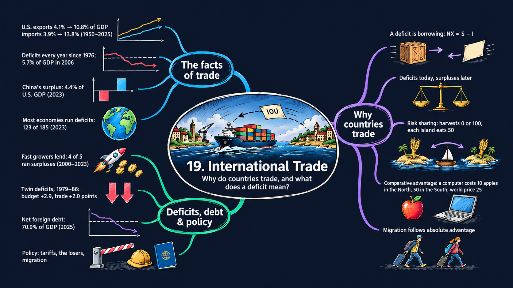
Learning goals

The United States buys more from the rest of the world than it sells to it, and it has done so every year since 1976. Is that a problem? This chapter looks at the facts of trade and at a few small examples that explain why countries trade at all. By the end of it you will be able to:

read the U.S. trade data: exports, imports and the trade balance (net exports) as shares of GDP;
derive \(NX = S - I\) step by step from the national income identity \(Y = C + I + G + NX\), explain why a trade deficit is borrowing from the rest of the world, and derive the country’s intertemporal budget constraint and the long-run foreign debt ratio from the way deficits add up to a foreign debt;
solve the textbook’s trade examples with algebra (exchange, trade across time, comparative advantage, free migration), derive the free-trade world price and the condition for specialization, read the comparative statics as elasticities, and say who gains from each arrangement;
compare trade balances across countries and periods, and check which year or which window a published number really refers to;
go beyond the textbook’s countries: pick any economy from World Bank, Penn World Table, IMF and External Wealth of Nations data, and check one source against another;
in Python: write small accounting functions once and reuse them, reshape tables with melt and pivot, draw grouped bar charts, average over a window with .loc[start:end], and add up flows with cumsum.

Model overview

Picture Islandia, the small island country we have followed through the book, and its large trading partner across the water, Mainland. Islanders sell fish to Mainland and buy many goods they do not make, and in some years they buy more than they sell. How does Islandia pay for the gap, and why trade at all with a partner that is better at almost everything? This section answers with a few accounting rules and four small trade models, with Islandia in view throughout.

The big idea

The question. Why do countries trade, and what does it mean when a country buys more from abroad than it sells?

The answer in one sentence. A trade deficit is borrowing from abroad, which must be repaid in present value, and trade pays off because each country can specialize in its comparative advantage.

What goes in and what comes out. The accounting takes spending, taxes, the return \(\bar{r}\) and the growth rate \(\bar{g}\), and gives back the trade balance, the saving–investment gap and the foreign debt. The trade models take endowments, productivities and labor forces, and give back prices, wages, who makes what and who consumes how much.

Road map.

The trade balance and the national income identity: what a deficit means.
Saving, investment and the trade balance: a deficit seen as borrowing, and the twin deficits.
Net foreign assets and the intertemporal budget constraint: how deficits pile up into a debt, and why they must be repaid.
Gains from exchange: two islands, two goods: trade with no production at all.
Trade across time: Oddtopia and Eventopia: deficits and surpluses as loans.
Comparative advantage: the North and the South: autarky, free trade and who gains.
Free migration: moving workers instead of goods: what happens when people move instead of goods.
Model in code: every rule as a Python function, checked with numbers.

Notation. Capital letters are flows of goods during a year, and lower-case letters are the same flows divided by GDP, such as \(c = C/Y\). A bar marks a parameter, picked from outside; letters without a bar are endogenous variables.

Symbol	Meaning	Type
\(Y, C, I, G, T\)	output, consumption, investment, government purchases and taxes	endogenous
\(EX, IM, NX\)	exports, imports and net exports (the trade balance)	endogenous
\(S\)	domestic saving, private plus government	endogenous
\(c, i, g, nx\)	\(C\), \(I\), \(G\) and \(NX\) as fractions of GDP	notation
\(F_t, CA_t\)	net foreign assets at the end of year \(t\), and the current account	endogenous
\(f_t, f^*\)	net foreign assets as a fraction of GDP, and its long-run value	endogenous
\(\bar{r}\)	the return on foreign assets	parameter
\(\bar{g}\)	the growth rate of nominal GDP	parameter
\(x_j, z_j, L_j\)	apples or computers per worker, and workers, in country \(j\)	parameters
\(w, p, c_A, c_C\)	the wage and the price of a computer (both in apples), and apples and computers per person	endogenous
\(n, s\)	subscripts for the North and the South	notation

The trade balance and the national income identity

Definitions

Exports \(EX\) are goods and services made at home and bought by buyers in other countries: the fish that Islandia sells on Mainland. Imports \(IM\) go the other way: goods and services made abroad and bought at home, whether by households, firms or the government.
The trade balance, or net exports, is \(NX \equiv EX - IM\). When it is positive, the country runs a trade surplus; when it is negative, a trade deficit.
The share of GDP of a flow \(X\) is \(100 \times X/Y\) (Appendix C.2). Shares let us draw a tiny and a huge economy, or the year 1950 and the year 2025, on one axis.
The national income identity divides production among its uses: \(Y = C + I + G + NX\). Why net exports, and not exports alone? The spending \(C + I + G\) also buys goods made abroad, which are no part of domestic production, so imports come out. Goods made at home and shipped abroad are part of production, but no domestic buyer spends on them, so exports go in. That gives \(Y = (C + I + G) + EX - IM\).

Solving the identity

Step 1: net exports as production minus domestic spending. Take \(C + I + G\) away from both sides of the identity:

\[NX = Y - (C + I + G).\]

The sum \(C + I + G\) is all that households, firms and the government use at home. Economists call it domestic absorption. The equation splits into two cases:

\[NX < 0 \;\Longleftrightarrow\; C + I + G > Y, \qquad\qquad NX > 0 \;\Longleftrightarrow\; C + I + G < Y.\]

In words

In a deficit year, islanders use more goods than they make. The extra goods come from Mainland, which takes a promise of payment in return. To keep that promise, Islandia must later make more than it uses, and the inequality turns around.

Step 2: the same identity in shares of GDP. Divide each term by \(Y\):

\[\frac{NX}{Y} = \frac{Y}{Y} - \frac{C}{Y} - \frac{I}{Y} - \frac{G}{Y} \qquad\Longrightarrow\qquad nx = 1 - c - i - g.\]

The Penn World Table gives the shares \(c\), \(i\) and \(g\), but not \(nx\), so this formula is how we compute the trade balances of Figs. 3 and 4. Shares of \(c = 0.55\), \(i = 0.25\) and \(g = 0.18\), for instance, sum to \(0.98\), and the remaining 2 percent of GDP is a surplus.

Key result: the trade balance identity

\[NX = Y - (C + I + G) \tag{1}\]

\[nx = 1 - c - i - g \tag{2}\]

The trade balance is production minus domestic use, in levels (1) or in shares of GDP (2).

Islandia in numbers. Take the economy of Check 1 in Model in code: \(Y = 100\), \(C = 70\), \(I = 20\) and \(G = 15\). Then \(NX = 100 - 105 = -5\), a trade deficit of 5 percent of GDP.

Step 3: the world as a whole. Divide the world into two regions, the United States (US) and the rest of the world (RoW). Whatever the United States imports, the rest of the world exports, and the other way round: \(IM_{US} = EX_{RoW}\) and \(EX_{US} = IM_{RoW}\). So

\[NX_{US} = EX_{US} - IM_{US} = IM_{RoW} - EX_{RoW} = -NX_{RoW}.\]

Nobody outside the world buys from it, so all countries’ trade balances add up to zero. To see which countries finance the U.S. deficit, we must measure everything against one GDP. Multiply and divide by the GDP \(Y_j\) of country \(j\):

\[\frac{NX_j}{Y_{US}} = \frac{NX_j}{Y_j}\times\frac{Y_j}{Y_{US}}.\]

That is the second bar of Fig. 3. An economy three quarters as large as the United States, with a surplus of 2 percent of its own GDP, covers \(2 \times 0.75 = 1.5\) percent of U.S. GDP.

What the identity predicts

An identity says nothing about cause and effect. It only says which numbers can go together. Holding output \(Y\) fixed:

A change in …	effect on the trade balance
\(C\), \(I\) or \(G\) up by 1	\(NX\) down by 1
\(c + i + g\) up by 1 point of GDP	\(nx\) down by 1 point
U.S. deficit up by 1 point of U.S. GDP	surpluses elsewhere up by 1 point of U.S. GDP in total

Each effect is one for one, since the identity is just a sum. The direction of cause stays open: a boom in spending at home can create a deficit, and easy credit from abroad can also fuel a boom in spending. The models below, and the data sections, help us judge which story fits.

A trade deficit means a country uses more goods than it makes, and the missing goods arrive from abroad on credit.

Check your understanding

1. Islandia produces \(Y = 100\), with \(C = 70\), \(I = 20\) and \(G = 15\). What is its trade balance, as a share of GDP? What would it be if the government cut its purchases to \(G = 10\), with everything else unchanged?

Answer

By equation (1), \(NX = 100 - (70 + 20 + 15) = -5\): a deficit of 5 percent of GDP. With \(G = 10\), domestic uses add up to exactly 100, so \(NX = 0\) and trade is balanced.

2. Islandia’s deficit grows by 1 point of GDP. Can we conclude from the identity that islanders began to overspend?

Answer

No. Equation (2) says only that \(c + i + g\) rose by 1 point. It does not say why: islanders may have chosen to spend more, or cheap loans from Mainland may have pulled spending up. The identity holds in both stories.

Saving, investment and the trade balance

Definitions

Private saving is income after taxes, minus consumption: \(Y - T - C\). As in Chapter 18, \(T\) stands for taxes net of transfers.
Government saving is the budget surplus \(T - G\) (for Islandia, the surplus of the Islandia Treasury). It turns negative when the government runs a deficit.
Foreign saving is \(IM - EX = -NX\): the goods the rest of the world sends us in excess of what we send back. That excess is a loan to us.
Domestic saving is the sum of the first two: \(S \equiv (Y - T - C) + (T - G)\).

Solving the identity

Step 1. Solve the national income identity for investment: \(I = Y - C - G - NX\).

Step 2. Take taxes away and add them back, which leaves the value unchanged: \(I = (Y - T - C) + (T - G) - NX\).

Step 3. Replace \(-NX\) by \(IM - EX\):

\[I = \underbrace{(Y - T - C)}_{\text{private saving}} + \underbrace{(T - G)}_{\text{government saving}} + \underbrace{(IM - EX)}_{\text{foreign saving}}.\]

Each unit of investment has one of three sources of funds: households, the government or foreigners.

Step 4. Inside domestic saving the taxes cancel: \(S = (Y - T - C) + (T - G) = Y - C - G\). So the equation of Step 1 is \(I = S - NX\). Move \(NX\) to the left and \(I\) to the right, and the trade balance appears as the gap between saving and investment.

Key result: saving, investment and the trade balance

\[I = (Y - T - C) + (T - G) + (IM - EX) \tag{3}\]

\[NX = S - I \tag{4}\]

Investment is paid for by private, government and foreign saving (3). The trade balance equals the net capital outflow \(S - I\), the net amount a country lends to the rest of the world (4).

Islandia in numbers. Add taxes \(T = 12\) to the economy above. Private saving is \(100 - 12 - 70 = 18\), government saving is \(12 - 15 = -3\), and foreign saving is 5. Together they pay for \(I = 20\). Domestic saving is \(S = 15\), so \(S - I = -5\), the same as \(NX\).

In words: one deal, two sides

Equation (4) tells one story twice. On the goods side, Islandia receives more from Mainland than it ships, \(NX < 0\). On the money side, islanders save less than they invest, \(S < I\), and Mainland lends them the gap in exchange for bonds, shares or money. A deficit and foreign borrowing are the same deal.

Step 5: the twin deficits. Break domestic saving into its two parts:

\[NX = \underbrace{(Y - T - C - I)}_{\text{private saving minus investment}} + \underbrace{(T - G)}_{\text{government saving}}.\]

Suppose private saving and investment move roughly together, so that the first term stays near zero. Then the trade balance tracks the budget balance: a budget deficit goes with a trade deficit of about the same size. These are the twin deficits of Fig. 5.

What the identity predicts

Equation (4) is true every year, but it does not say which term gives way. The table lists the cases, each for a change of 1 point of GDP:

A change in …	holding fixed …	effect
budget deficit \(G - T\) up	private saving and \(I\)	\(NX\) down by 1: the twin deficits
budget deficit \(G - T\) up	private saving and \(NX\)	\(I\) down by 1: crowding out at home
investment \(I\) up	\(S\)	\(NX\) down by 1: foreigners finance it
private saving up	\(I\) and \(T - G\)	\(NX\) up by 1: the country lends abroad

This matters for two of the data sections. A fast-growing country that invests a lot can still have a trade surplus, as long as it saves even more, as China does (Fig. 4). And when the U.S. budget deficits were large, in the 1980s and the 2000s, they came mostly with larger trade deficits, not with lower investment (Fig. 5).

Investment is financed by households, the government or foreigners, and a trade deficit is simply the foreigners’ share.

Check your understanding

1. In the Islandia example, private saving is 18, investment is 20 and taxes are 12. The Islandia Treasury raises its purchases from 15 to 17, and private saving and investment stay the same. What happens to the trade balance?

Answer

By Step 5, \(NX = (18 - 20) + (12 - 17) = -2 - 5 = -7\). The trade deficit grows from 5 to 7 percent of GDP, one for one with the budget deficit: the twin deficits.

2. Islanders build many new boats, and yet Islandia runs a trade surplus. Is that a contradiction?

Answer

No. By equation (4), \(NX = S - I\). High investment and a surplus go together whenever saving is higher still. The extra saving is then lent to Mainland. The fast-growing economies of Fig. 4 show exactly this pattern.

Net foreign assets and the intertemporal budget constraint

Definitions

A country’s net foreign assets \(F_t\) are what its residents own abroad, minus what foreigners own in the country, at the end of year \(t\). In the data this is the net international investment position (Fig. 6). If \(F_t < 0\), then \(-F_t\) is the net foreign debt: what Islandia owes Mainland, net.
The current account is the trade balance plus the net income on foreign assets: \(CA_t \equiv NX_t + \bar{r}F_{t-1}\), with \(\bar{r}\) the return on those assets. (Remittances and aid also enter the data; we leave them out.) The textbook’s trade examples set this income to zero, so there the current account and the trade balance coincide.

Solving the model

Step 1: assets pile up the current account. A current account surplus is a new loan to the rest of the world, so the stock of foreign assets rises by that amount:

\[F_t - F_{t-1} = NX_t + \bar{r}F_{t-1} \qquad\Longrightarrow\qquad F_t = (1 + \bar{r})F_{t-1} + NX_t.\]

This is a difference equation (Appendix C.10). When \(\bar{r} = 0\), as in the island example below and the dotted line of Fig. 6, it reduces to \(F_t = F_{t-1} + NX_t\). Then \(F_t = F_0 + NX_1 + NX_2 + \dots + NX_t\): today’s stock is the first stock plus every trade balance since.

Step 2: the budget constraint over many years. Divide both sides by \((1 + \bar{r})^t\), and note that \((1 + \bar{r})/(1 + \bar{r})^t = 1/(1 + \bar{r})^{t-1}\):

\[\frac{F_t}{(1 + \bar{r})^t} = \frac{F_{t-1}}{(1 + \bar{r})^{t-1}} + \frac{NX_t}{(1 + \bar{r})^t}.\]

Write this line once for each year \(t = 1, 2, \dots, T\), and add up all the lines. Every term \(F_t/(1+\bar{r})^t\) with \(t\) between 1 and \(T - 1\) shows up once on each side and cancels. Only the first and the last stock remain:

\[\frac{F_T}{(1 + \bar{r})^T} = F_0 + \sum_{t=1}^{T}\frac{NX_t}{(1 + \bar{r})^t}.\]

Lenders do not let a debt grow forever without being repaid, and no country ships goods to the world forever without ever cashing its claims. So, far enough ahead, the final stock is worth zero today, \(F_T/(1 + \bar{r})^T = 0\), and the trade balances must cover the starting stock.

Key result: foreign assets and the budget constraint

\[F_t = (1 + \bar{r})F_{t-1} + NX_t \tag{5}\]

\[\sum_{t=1}^{T}\frac{NX_t}{(1 + \bar{r})^t} = -F_0 \tag{6}\]

Equation (5) moves foreign assets from year to year. Equation (6) is the intertemporal budget constraint: in present value, future trade balances must repay the starting debt.

The left-hand side of (6) is a sum of present values (Appendix C.12). It is the same algebra as the government’s budget constraint in Chapter 18, applied now to a whole country.

In words

If Islandia starts owing Mainland nothing, \(F_0 = 0\), its trade balances must be worth zero in present value: each deficit today needs later surpluses of equal present value. If it starts in debt, \(F_0 < 0\), it must run surpluses on average.

Step 3: foreign debt as a share of GDP. Let GDP grow at the rate \(\bar{g}\), so that \(Y_t = (1 + \bar{g})Y_{t-1}\), and define \(f_t \equiv F_t/Y_t\). Dividing equation (5) by \(Y_t\) gives

\[f_t = \frac{(1 + \bar{r})F_{t-1}}{(1 + \bar{g})Y_{t-1}} + \frac{NX_t}{Y_t} = \frac{1 + \bar{r}}{1 + \bar{g}}\,f_{t-1} + nx_t.\]

When GDP grows faster than the return, \(\bar{g} > \bar{r}\), the coefficient on \(f_{t-1}\) is less than one. With a constant trade balance \(nx\), the ratio then comes to rest. At rest \(f_t = f_{t-1} = f^*\), so \(f^* - \frac{1 + \bar{r}}{1 + \bar{g}}f^* = nx\), that is \(f^*\,\frac{\bar{g} - \bar{r}}{1 + \bar{g}} = nx\). Solving for \(f^*\):

Key result: the long-run foreign debt ratio

\[f^* = \frac{(1 + \bar{g})\,nx}{\bar{g} - \bar{r}} \tag{7}\]

A steady deficit leads to a stable debt ratio, as long as GDP grows faster than the return on the debt.

Islandia in numbers. \(F\) and \(Y\) are both in money, so \(\bar{g}\) is the growth of nominal GDP. If Islandia runs a deficit of 3 percent of GDP every year, \(nx = -0.03\), while nominal GDP grows at \(\bar{g} = 0.04\) and \(\bar{r} = 0\), then \(f^* = 1.04 \times (-0.03)/0.04 = -0.78\): a net foreign debt of 78 percent of GDP.

The U.S. debt in Fig. 6, about 70 percent of GDP, is of the same order.

What the model predicts

Deficits are loans, and they accumulate. By equation (5), the foreign debt is roughly the sum of past current account deficits. Fig. 6 checks this. It also reveals a second source of change in the data: foreign assets gain or lose value as stock prices and the dollar move.
Over time, trade must balance in present value. By equation (6), deficits cannot last forever. A deficit is a promise of surpluses to come, not goods for free.
Comparative statics of the debt ratio, from equation (7):

A rise in …	effect on the long-run ratio \(f^*\)	with \(nx = -0.03\), \(\bar{g} = 0.04\), \(\bar{r} = 0\)
the deficit \(-nx\), by 1 point	debt up by \((1+\bar{g})/(\bar{g}-\bar{r})\) points; the elasticity with respect to \(nx\) is 1	about 26 points more debt
the growth rate \(\bar{g}\)	debt ratio smaller: the same deficit is spread over a larger economy	\(\bar{g} = 0.05\): debt of 63 percent instead of 78
the return \(\bar{r}\) (below \(\bar{g}\))	debt ratio larger: interest on the debt adds to the borrowing	\(\bar{r} = 0.02\): debt of 156 percent

Deficits add up to a foreign debt, and in present value later surpluses must pay it back.

Check your understanding

1. Islandia keeps its deficit at 3 percent of GDP with \(\bar{r} = 0\), but its nominal GDP now grows at 5 percent a year instead of 4. Where does its foreign debt ratio settle?

Answer

By equation (7), \(f^* = 1.05 \times (-0.03)/0.05 = -0.63\): a net foreign debt of 63 percent of GDP, down from 78 percent. The same yearly deficit is spread over an economy that grows faster.

2. Islandia owes Mainland money, and the return \(\bar{r}\) is positive. Last year its trade was balanced, yet its foreign debt grew. How can that be?

Answer

Equation (5) adds the interest \(\bar{r}F_{t-1}\) to the trade balance. With \(F_{t-1} < 0\) that term is negative, so the current account is in deficit even with \(NX = 0\), and the debt grows. In the data, changes in the value of foreign assets can also move \(F_t\) (Fig. 6).

Gains from exchange: two islands, two goods

Assumptions

Two islands have equal populations. Everyone eats bananas and fish, and only in equal amounts: one meal is one banana together with one fish.
Nobody produces anything. Every year, each person on island 1 gets 200 bananas and 800 fish, and each person on island 2 gets the opposite, 800 bananas and 200 fish.
The islands may swap goods. Since the setup is symmetric, the swap is one fish for one banana.

Solving the model

Without trade, a person on island 1 can make only \(\min(200, 800) = 200\) meals, and the other 600 fish are useless. Now let island 1 give \(q\) fish for \(q\) bananas. It ends with \(200 + q\) bananas and \(800 - q\) fish. Meals need equal amounts, so

\[200 + q = 800 - q \quad\Longrightarrow\quad 2q = 600 \quad\Longrightarrow\quad q = 300.\]

Everyone on both islands ends with 500 bananas and 500 fish.

Key result: the gains from exchange

With endowments \((a, b)\) on one island and \((b, a)\) on the other, the swap is

\[q = \frac{b - a}{2},\]

and everyone ends with \((a + b)/2\) of each good. Meals per person rise from \(\min(a, b)\) to \((a + b)/2\).

The two islands in numbers. With \(a = 200\) and \(b = 800\), the islands swap 300 fish for 300 bananas, and meals per person rise from 200 to 500.

In words

Picture Islandia as island 1: its fishers land more fish than islanders can eat, while bananas are scarce. A fish is worth little at home and a lot on the other island. The swap moves each good to the people who value it most, and both islands gain without one more fish caught.

What the model predicts

Both islands are better off. Meals per person go from 200 to 500 on each island, and nothing extra is produced. The whole gain comes from sending each good to the people who value it more at the margin.
Trade here is balanced. Each island ships as much as it receives every year, so \(NX = 0\). The next block shows where deficits and surpluses come from.
Trade between countries is like trade between people. Inside a country, people specialize and buy most of what they use from others. Trade across borders takes the same idea one step further.

Swapping goods can make everyone better off even when nothing more is produced.

Check your understanding

1. Suppose each person on island 1 receives 300 bananas and 700 fish, and each person on island 2 receives 700 bananas and 300 fish. How much do the islands swap, and how many meals does each person get with and without trade?

Answer

By the Key result, \(q = (700 - 300)/2 = 200\). Everyone ends with 500 bananas and 500 fish, so meals rise from 300 to 500 per person.

2. No new good is made. Where, then, does the gain come from?

Answer

From moving goods to where they are worth more. On island 1 an extra fish adds no meal, but on island 2 it completes a meal. The swap uses goods that were idle before. Each island ships as much as it receives, so trade stays balanced, \(NX = 0\).

Trade across time: Oddtopia and Eventopia

Assumptions

The only good is wheat, and wheat cannot be kept from one year to the next.
Oddtopia harvests 100 bushels in odd years and none in even years. Eventopia harvests in the opposite years.
People like a smooth path of consumption better than one that jumps up and down. With diminishing marginal utility, the last bushel eaten in a rich year is worth less than the first bushel in a poor year (consumption smoothing, as in Chapter 16).
Nobody invests and there is no government, \(I = G = 0\). A bushel lent this year comes back as one bushel next year, so \(\bar{r} = 0\). Neither island starts with foreign assets, \(F_0 = 0\).

Solving the model

Step 1: the trade balance. With \(I = G = 0\), equation (1) reads \(NX_t = Y_t - C_t\): the harvest minus what is eaten.

Step 2: consumption. Together the islands harvest 100 bushels each year. Wheat cannot be stored, so all 100 bushels are eaten in the year they grow. The smoothest way to share a constant total, the same in every year, is 50 bushels per island: \(C_t = 50\).

Step 3: the trade balances. Oddtopia’s trade balance is \(NX_t = 100 - 50 = +50\) in odd years and \(NX_t = 0 - 50 = -50\) in even years. Eventopia’s is the mirror image. So the two balances sum to zero every year, just as Step 3 of the first block says they must.

Step 4: the assets. Equation (5) with \(\bar{r} = 0\) and \(F_0 = 0\) gives Oddtopia’s net foreign assets: \(F_1 = 50\), \(F_2 = 50 - 50 = 0\), \(F_3 = 50\), and so on. After each good harvest Oddtopia holds a claim of 50 bushels on Eventopia, and the claim is repaid a year later. Eventopia’s assets run \(-50, 0, -50, \dots\)

Step 5: the budget constraint. With \(\bar{r} = 0\) and \(F_0 = 0\), equation (6) requires the trade balances to sum to zero. Over every pair of years they do: \(+50 - 50 = 0\).

Key result: trade as lending across time

Each island eats \(C_t = 50\) bushels every year. Oddtopia’s trade balance alternates between \(+50\) and \(-50\), and its net foreign assets between 50 and 0. Eventopia mirrors it, and every two years each island’s balances sum to zero, as equation (6) requires.

In words

Islandia’s catch has good and bad seasons too. In a good season it ships fish to Mainland and keeps the claims; in a bad one it cashes them and runs a deficit. That deficit is no sign of trouble: it keeps islanders fed when the nets come back empty.

What the model predicts

Sharing risk. Each island eats 50 bushels a year, although its own harvest jumps between 0 and 100. Without trade, it would alternate between feast and famine.
A deficit can raise welfare. Each island has a deficit in exactly the years when its harvest fails. The deficit is a loan that keeps it fed.
Balanced on average. Each island’s average trade balance is zero, as equation (6) requires. Today’s deficit is the other side of tomorrow’s surplus.
A guide to the data. By the same logic, a country should borrow, and so run deficits, when its income is low for a while, when it expects to grow faster than the rest of the world, or when it has good projects to invest in. Fig. 4 asks whether countries that grow fast really do borrow.

A deficit can be a loan that smooths consumption, and over time it is balanced by later surpluses.

Check your understanding

1. Suppose Oddtopia harvests 80 bushels in odd years and 20 in even years, and Eventopia the reverse. What does each island eat, and what are Oddtopia’s trade balance and foreign assets in years 1 and 2?

Answer

The world still harvests 100 bushels a year, so each island eats 50. By Step 1, Oddtopia’s trade balance is \(80 - 50 = +30\) in year 1 and \(20 - 50 = -30\) in year 2. By equation (5) with \(\bar{r} = 0\), its assets are \(F_1 = 30\) and \(F_2 = 0\).

2. In an even year, Oddtopia runs a large trade deficit. Is that bad news?

Answer

No. The deficit is the repayment of last year’s loan by Eventopia, in wheat, and it lets Oddtopia eat 50 bushels in a year with no harvest. Over any two years its trade balances add up to zero, as equation (6) requires.

Comparative advantage: the North and the South

Assumptions

Two countries, the North (\(n\)) and the South (\(s\)), make and consume two goods: apples and computers. Labor is the only input. Each worker supplies one unit of labor for a wage \(w\), and the wage is all of the worker’s income.
In country \(j\) there are \(L_j\) workers, and each can make either \(x_j\) apples or \(z_j\) computers. We use the textbook’s numbers throughout this notebook:

	North	South
workers \(L\)	100	400
apples per worker \(x\)	160	100
computers per worker \(z\)	16	2

Inside its own country, a worker can move freely between the two sectors, but nobody crosses the border (the migration block below lifts this rule).
Everybody spends half of income on apples and half on computers. Apples are the unit of account (the numéraire): an apple costs 1, and a computer costs \(p\) apples. Let \(c_A\) and \(c_C\) be the apples and computers that one person consumes. The two spending shares then give

\[\frac{1 \times c_A}{w} = \frac{1}{2} \;\;\text{and}\;\; \frac{p \times c_C}{w} = \frac{1}{2} \qquad\Longrightarrow\qquad c_A = \frac{w}{2}, \qquad c_C = \frac{w}{2p}. \tag{8}\]

The North makes more of both goods per worker, \(x_n > x_s\) and \(z_n > z_s\): it has an absolute advantage in both. But its edge is far larger in computers, \(z_n/z_s = 16/2 = 8\), than in apples, \(x_n/x_s = 160/100 = 1.6\). Cross-multiplying, \(z_n/z_s > x_n/x_s\) is the same as \(x_s/z_s > x_n/z_n\). To make one computer, the North gives up \(160/16 = 10\) apples and the South \(100/2 = 50\). Computers cost relatively less to make in the North, so the North has a comparative advantage in computers, and the South in apples.

Solving the model: autarky

In autarky, neither country trades.

Step 1: the wage. A worker who grows apples makes \(x\) of them, at a price of 1 each, so the wage is \(w = x\).

Step 2: the price of a computer. A worker who makes computers makes \(z\) of them and earns \(p\,z\) apples. People want both goods, so both sectors need workers, and so both must pay the same wage: \(p\,z = x\). If computers paid more, all workers would leave the orchards; if they paid less, nobody would make computers. The price of a computer is therefore \(p = x/z\), its opportunity cost: the apples given up to make it (Appendix C.9 on solving such conditions).

Step 3: consumption. Put \(w = x\) and \(p = x/z\) into equation (8): \(c_A = x/2\) and \(c_C = \dfrac{x/2}{x/z} = \dfrac{z}{2}\).

Step 4: who works where. The \(L_A\) apple growers produce \(L_A\,x\) apples, and the \(L\) people eat \(L\,x/2\). Equating the two gives \(L_A = L/2\): half of the workers grow apples, and half make computers.

Key result: autarky

\[w = x, \qquad p = \frac{x}{z} \tag{9}\]

Each person consumes \(c_A = x/2\) apples and \(c_C = z/2\) computers, and half of the workers are in each sector.

The North and the South in numbers. The North has \(w = 160\) and \(p = 10\), and each person consumes 80 apples and 8 computers. The South has \(w = 100\) and \(p = 50\), and each person consumes 50 apples and 1 computer.

In total, the North makes \(50 \times 160 = 8{,}000\) apples and \(50 \times 16 = 800\) computers, and the South makes \(200 \times 100 = 20{,}000\) apples and \(200 \times 2 = 400\) computers.

Solving the model: free trade

Step 1: arbitrage. In autarky a computer costs 10 apples in the North but 50 in the South. A trader could buy computers in the North and resell them in the South at a profit (arbitrage). Under free trade such gaps vanish, and there is a single world price \(p\).

Step 2: a guess. Suppose each country makes only the good of its comparative advantage: the North only computers, the South only apples. World output is then \(L_n z_n = 1{,}600\) computers and \(L_s x_s = 40{,}000\) apples.

Step 3: the world price. World income in apples is the value of all output, \(L_s x_s + p\,L_n z_n\). Half of it buys computers, and in equilibrium the computers bought are the computers made:

\[p\,L_n z_n = \tfrac{1}{2}\left(L_s x_s + p\,L_n z_n\right) \quad\Longrightarrow\quad \tfrac{1}{2}\,p\,L_n z_n = \tfrac{1}{2}\,L_s x_s \quad\Longrightarrow\quad p = \frac{L_s x_s}{L_n z_n}.\]

Because people spend equal shares on the two goods, world apples and world computers must be worth the same in total. The price of a computer is therefore world apples divided by world computers: \(40{,}000/1{,}600 = 25\) apples.

Step 4: wages. A southern worker still grows 100 apples, so \(w_s = x_s = 100\). A northern worker makes 16 computers worth 25 apples each, so \(w_n = p\,z_n = 400\) apples. With the formula for \(p\), \(w_n = L_s x_s/L_n\).

Step 5: consumption. Equation (8) gives, in the North, \(c_A = 400/2 = 200\) and \(c_C = 400/(2 \times 25) = 8\); in the South, \(c_A = 100/2 = 50\) and \(c_C = 100/(2 \times 25) = 2\).

Step 6: check the guess. Northern workers keep making computers only if computers pay at least as much as apples, \(p\,z_n \ge x_n\), or \(p \ge x_n/z_n\). Southern workers keep growing apples only if \(x_s \ge p\,z_s\), or \(p \le x_s/z_s\). With strict inequalities, both countries specialize completely when the world price sits strictly between the two autarky prices.

Key result: free trade

\[p = \frac{L_s x_s}{L_n z_n} \tag{10}\]

\[\frac{x_s}{z_s} \;>\; p = \frac{L_s x_s}{L_n z_n} \;>\; \frac{x_n}{z_n} \tag{11}\]

The world price (10) is the ratio of world apples to world computers. Complete specialization requires it to lie between the two autarky prices (11).

The North and the South in numbers. \(p = 40{,}000/1{,}600 = 25\) apples, and \(50 > 25 > 10\), so the guess is right. The northern wage is 400 apples and the southern wage 100.

If, say, the South were large enough to push \(p\) above 50, some southern workers would also make computers, and the South would keep its autarky price.

In words: why Islandia trades with a stronger partner

Suppose Mainland is better than Islandia at both fishing and making machines. Trade still pays for both, because what counts is what each side gives up. If Islandia is a little worse at fishing but much worse at machines, a machine costs it many fish at home, and buying it from Mainland is cheaper.

What the model predicts

Both countries gain, for any numbers that satisfy (11). Compare each item of consumption under autarky and free trade:

	autarky	free trade	comparison
North, apples	\(x_n/2 = 80\)	\(p\,z_n/2 = 200\)	higher, because \(p > x_n/z_n\)
North, computers	\(z_n/2 = 8\)	\(w_n/(2p) = z_n/2 = 8\)	the same
South, apples	\(x_s/2 = 50\)	\(x_s/2 = 50\)	the same
South, computers	\(z_s/2 = 1\)	\(x_s/(2p) = 2\)	higher, because \(p < x_s/z_s\)

Each country gets more of the good it imports, and no less of the good it makes. What drives trade is comparative advantage: the North gains although it is better at everything. World output grows too, from \(28{,}000\) apples and \(1{,}200\) computers in autarky to \(40{,}000\) apples and \(1{,}600\) computers.

Comparative statics. Take logs of the free-trade results (Appendix C.4), for instance \(\ln p = \ln L_s + \ln x_s - \ln L_n - \ln z_n\), and each coefficient is an elasticity. They are valid as long as condition (11) holds:

A 1% rise in …	\(p = \frac{L_s x_s}{L_n z_n}\)	\(w_n\), North apples \(= \frac{L_s x_s}{2L_n}\)	North computers \(= \frac{z_n}{2}\)	South apples \(= \frac{x_s}{2}\)	South computers \(= \frac{L_n z_n}{2L_s}\)
\(z_n\) (northern computers)	\(-1\%\)	\(0\)	\(+1\%\)	\(0\)	\(+1\%\)
\(x_s\) (southern apples)	\(+1\%\)	\(+1\%\)	\(0\)	\(+1\%\)	\(0\)
\(L_n\) (northern workers)	\(-1\%\)	\(-1\%\)	\(0\)	\(0\)	\(+1\%\)
\(L_s\) (southern workers)	\(+1\%\)	\(+1\%\)	\(0\)	\(0\)	\(-1\%\)

When the North gets better at making computers, computers become cheaper everywhere. The northern wage in apples stays put, because each computer now buys fewer apples, and the South gains just as many computers as the North. Prices spread productivity gains across borders. With \(z_n = 20\), for example, the world price drops to \(40{,}000/2{,}000 = 20\) apples, and condition (11) still holds, \(50 > 20 > 8\).

Trade follows comparative advantage, so even a country that is better at everything gains from it.

Check your understanding

1. The North’s computer productivity rises to \(z_n = 20\), and nothing else changes. Find the world price, the northern wage, and what one person consumes in each country.

Answer

By equation (10), \(p = 40{,}000/(100 \times 20) = 20\) apples, and condition (11) still holds, \(50 > 20 > 8\). The northern wage is \(w_n = 20 \times 20 = 400\) apples, unchanged. By equation (8), a northerner consumes 200 apples and \(400/40 = 10\) computers, and a southerner 50 apples and \(100/40 = 2.5\) computers. Both countries get 25 percent more computers.

2. The South is less productive than the North in both goods. Why does it still gain from trade?

Answer

Because what matters is the opportunity cost. A computer costs the South 50 apples at home (equation 9), but only 25 apples on the world market (equation 10). By growing apples and buying computers, each southerner gets 2 computers instead of 1, with the same 50 apples.

Free migration: moving workers instead of goods

Assumptions

Keep the North–South model, but now let workers cross the border. Technology stays put: in the North, any worker makes \(x_n\) apples or \(z_n\) computers, wherever he or she was born. Production has constant returns, so output per worker does not depend on how many workers a country has.

Solving the model

Step 1: who moves. Under free trade a computer costs the same everywhere, so a higher wage in apples means a higher real wage. The northern wage, 400 apples, is four times the southern wage of 100 apples (in autarky it is 160 against 100). Southern workers keep moving while any gap is left. The North is more productive in both goods, so a worker makes more of either good there, and in the end the South is empty.

Step 2: the new world economy. The world now looks like the North in autarky, with \(L_n + L_s = 500\) workers. By equation (9), \(w = x_n = 160\) and \(p = x_n/z_n = 10\). By equation (8), each person eats \(c_A = 80\) apples and has \(c_C = 8\) computers.

Step 3: production. Half of the 500 workers make each good: \(250 \times 160 = 40{,}000\) apples and \(250 \times 16 = 4{,}000\) computers.

Key result: free migration

All workers end up in the North, which then works like a closed economy with \(L_n + L_s\) workers. By equations (8) and (9),

\[w = x_n, \qquad p = \frac{x_n}{z_n}, \qquad c_A = \frac{x_n}{2}, \qquad c_C = \frac{z_n}{2}.\]

The North and the South in numbers. Everyone earns 160 apples, a computer costs 10 apples, and each person has 80 apples and 8 computers. The world makes 40,000 apples and 4,000 computers.

In words

Moving goods lets each country use its own technology where it is relatively best. Moving people lets every worker use the best technology in the world. If Mainland’s workshops beat Islandia’s at everything, islanders who moved there would make more of every good, and they would keep most of the gain.

What the model predicts

Migration follows absolute advantage, while trade in goods follows comparative advantage. Workers go where productivity is highest, full stop.
The world produces more than under free trade: the same 40,000 apples, but 4,000 computers instead of 1,600.
The gains go to the migrants. What one worker consumes under each arrangement:

	autarky	free trade	free migration
a worker born in the North	80 apples, 8 computers	200 apples, 8 computers	80 apples, 8 computers
a worker born in the South	50 apples, 1 computer	50 apples, 2 computers	80 apples, 8 computers

Northern workers are back at their autarky bundle: with constant returns, the newcomers leave their productivity unchanged. So northerners like free trade better than free migration.

The North could be compensated. Going from free trade to free migration, each of the 100 northerners loses 120 apples, 12,000 apples in all. Each of the 400 migrants gains 30 apples and 6 computers, 12,000 apples and 2,400 computers in all. The gains exceed the losses. If each migrant handed 30 apples to the North, every northerner would be back at the free-trade bundle of 200 apples and 8 computers, and every migrant would still have 50 apples and 8 computers: four times the computers of free trade.
Moving labor or moving capital. The production and Solow models (Chapter 4, Chapter 5) showed that poor countries are poor mainly because of low total factor productivity, and much less because they lack capital. Sending capital to an economy with low productivity leaves that problem where it is. Letting workers move to where productivity is high goes to the root of it, which is why the potential gains from migration are so large.
The costs of trade. In the model, northern apple growers turn into computer makers overnight, and nobody loses. In real life, changing jobs takes time and new skills, so trade makes winners and losers inside each country. Since the winners gain more than the losers lose, the winners could in principle compensate the losers, for instance through retraining and a social safety net.

Free migration raises world output the most, but the gains go to the migrants unless they share them.

Check your understanding

1. Under free migration, how many apples must each of the 400 migrants hand to the North so that each of the 100 northerners is back at the free-trade bundle of 200 apples?

Answer

Each northerner has 80 apples and needs 120 more, so the North needs \(100 \times 120 = 12{,}000\) apples. Shared among 400 migrants, that is \(12{,}000/400 = 30\) apples each. Each migrant keeps 50 apples and 8 computers, still more than under free trade.

2. Why does free migration raise the world’s computer output from 1,600 to 4,000, while free trade does not?

Answer

Under free trade, the South’s 400 workers grow apples with their own technology. Under free migration, they work with the North’s technology, which makes 16 computers per worker instead of 2. Migration follows absolute advantage, so every worker uses the best technology, and the world’s output of computers rises.

Recap

A deficit means using more than you make: \(NX = Y - (C + I + G)\) (the basic facts, Fig. 3).
A deficit is borrowing: \(NX = S - I\) (Fig. 4), and budget deficits can bring twin deficits.
Deficits pile up into a foreign debt (5), are repaid in present value (6), and settle at a stable ratio to GDP when \(\bar{g} > \bar{r}\) (7) (foreign debt).
Trade moves goods to where they are worth most, and shares risk (Oddtopia and Eventopia).
Comparative advantage: under free trade the world price lies between the autarky prices, and both countries gain (the North and the South).
Free migration follows absolute advantage, raises world output most, and the gains go to the migrants (free migration).

Model in code

Now we turn the accounting rules and the trade models into Python. The section has three parts: the setup (folded, because it is the same in every chapter), the model as functions, and numerical checks that also recompute the textbook’s tables. Run its cells once, in order. Every later section of the notebook reuses them.

Setup

Run the setup cells once, before anything else. They load the Python libraries, give every chart the same look, store the address of the chapter’s data and define the helpers that only the book website needs. You can use the notebook without reading them; open the box if you are curious.

Show the setup code

The first cell loads the libraries and sets the look of the charts. Its comments explain each step.

# @title Setup: libraries, chart colors and the data location
# Text after a "#" is a comment: Python ignores it, it is there for human readers.

# Step 1: load the libraries. `import` loads a library, a toolbox written by
# other people, and `as np` gives it a short nickname, so the code stays short.
import numpy as np                    # numbers and arrays
import pandas as pd                   # data tables
import plotly.express as px           # quick charts from data tables
import plotly.graph_objects as go     # charts built piece by piece
import plotly.io as pio               # settings shared by every chart
# sliders, buttons and menus for the interactive figures
from ipywidgets import interact, IntSlider, FloatSlider, ToggleButtons, Dropdown, SelectMultiple, fixed

# Step 2: one light blue/green look for every chart
BLUE, TEAL, GREEN, GRAY = "#16528c", "#008070", "#7fb23a", "#8a96a3"
pio.templates.default = "plotly_white"
# the same chart size in Colab and on the website
pio.templates["plotly_white"].layout.update(width=860, height=480)
px.defaults.color_discrete_sequence = [BLUE, TEAL, GREEN, "#5aa0d8", "#0b4f47"]
WIDE = {"description_width": "initial"}         # show the full widget labels

# Step 3, Colab only: let Plotly charts appear inside the interactive widgets.
# `try` runs the indented lines; if the import fails (we are not in Colab),
# `except` skips them.
try:
    import google.colab
    google.colab.output.enable_custom_widget_manager()
except ImportError:
    pass                                        # not running in Colab: nothing to do

# Step 4: the data files of this chapter live in the book's GitHub repository
DATA_URL = "https://raw.githubusercontent.com/quarcs-lab/macro102-site/main/data/ch19/"

The website cannot run Python, so each interactive figure also gets a version with a precomputed slider. The next helper builds those versions. Run it and move on.

# @title Helper for the website versions (run this cell; you do not need to read it)
def slider_figure(make_figure, name, values, start, label=None):
    """Join precomputed versions of a figure with one slider (the website cannot run Python).

    Arguments
        make_figure : the function that draws the figure
        name        : the argument the slider moves
        values      : the values of that argument to precompute
        start       : the value shown first
        label       : the slider's label (the argument name if None)
    Returns
        one Plotly figure with all versions and a slider that shows one at a time
    """
    # Step 1: draw the figure once for every value
    figures = [make_figure(**{name: v}) for v in values]
    first = values.index(start)
    # Step 2: copy every curve into one figure; only the start value's are visible
    fig = go.Figure(layout=figures[first].layout)
    owner = []                          # which precomputed figure each trace is from
    for i, f in enumerate(figures):
        for trace in f.data:
            trace.visible = (i == first)
            fig.add_trace(trace)
            owner.append(i)
    # Step 3: one slider step per value: its curves, title, labels and shapes
    steps = []
    for i, f in enumerate(figures):
        layout = {"title": f.layout.title.to_plotly_json(),
                  "annotations": [a.to_plotly_json() for a in f.layout.annotations],
                  "shapes": [s.to_plotly_json() for s in f.layout.shapes]}
        visible = [o == i for o in owner]
        steps.append(dict(method="update", label=str(values[i]), args=[{"visible": visible}, layout]))
    fig.update_layout(sliders=[dict(active=first, steps=steps, pad=dict(t=60),
                                    currentvalue=dict(prefix=(label or name) + " = "))])
    return fig

Every figure of this chapter can also show other countries. On the website, the many-country versions get a menu of country groups, built by two more helpers.

# @title Helpers for the many-country website versions (run this cell; you do not need to read it)
# Step 1: two fixed groups of countries for the menus
G7 = ["U.S.", "Japan", "Germany", "France", "United Kingdom", "Italy", "Canada"]
EMERGING = ["China", "India", "Brazil", "Russia", "Mexico", "Indonesia", "Türkiye", "South Africa",
            "Saudi Arabia", "Argentina"]


def country_groups(regions, book):
    """The menu groups: the textbook's countries, the G7, large emerging economies, the World Bank regions.

    Arguments
        regions : a table with one row per country and the columns country and region
        book    : the countries the textbook shows
    Returns
        a dictionary from each group's name to its list of countries
    """
    # Step 2: the three fixed groups first, then one group per region, A to Z
    groups = {"Textbook": list(book), "G7": G7, "Large emerging": EMERGING}
    for region in sorted(regions.region.unique()):
        # the countries whose region is this one
        groups[region] = list(regions[regions.region == region].country)
    return groups


def group_menu(fig, groups, start, title):
    """Show one group of countries at a time, chosen from a menu above the chart.

    A trace belongs to the country named before ', ' in its legendgroup. Each group gets a y range that covers
    its values; in groups of more than 15 countries it leaves out extreme outliers (double-click the chart to
    show them).

    Arguments
        fig    : a Plotly figure with the traces of every country
        groups : the menu groups, from country_groups
        start  : the group shown first
        title  : the chart's title
    Returns
        the same figure, with the menu
    """
    # Step 3: the country of each trace
    owners = [t.legendgroup.split(", ")[0] for t in fig.data]
    # Step 4: one menu entry per group: its traces and a y range that fits them
    buttons = []
    for name, members in groups.items():
        visible = [o in members for o in owners]   # the traces of this group
        # all their y values, without the missing ones (or a single 0 if none)
        ys = np.concatenate([np.asarray(t.y, dtype=float) for t, v in zip(fig.data, visible) if v]
                            or [np.zeros(1)])
        ys = ys[np.isfinite(ys)] if np.isfinite(ys).any() else np.zeros(1)
        lo, hi = ys.min(), ys.max()
        # large groups: leave out extreme outliers
        if len(set(o for o, v in zip(owners, visible) if v)) > 15:
            q5, q95 = np.percentile(ys, [5, 95])
            lo, hi = max(lo, q5 - 0.3 * (q95 - q5)), min(hi, q95 + 0.3 * (q95 - q5))
        pad = 0.06 * (hi - lo) + 0.5                # a little room above and below
        buttons.append(dict(label=name, method="update",
                            args=[{"visible": visible},
                                  {"yaxis.range": [lo - pad, hi + pad], "yaxis.autorange": False}]))
    # Step 5: start with the group `start`, and put the menu above the chart
    first = list(groups).index(start)
    for t, v in zip(fig.data, buttons[first]["args"][0]["visible"]):
        t.visible = v
    # the title, the start group's y range and the menu at the top left
    fig.update_layout(title=title, yaxis_range=buttons[first]["args"][1]["yaxis.range"], yaxis_tickvals=None,
                      margin=dict(t=115), updatemenus=[dict(buttons=buttons, active=first, direction="down",
                                                             x=0, y=1.02, xanchor="left", yanchor="bottom")])
    return fig

The last helper is like slider_figure, but with a drop-down menu instead of a slider.

# @title Helper for the website versions with a menu of countries (run this cell; you do not need to read it)
def menu_figure(make_figure, name, values, start):
    """Like slider_figure, but with a drop-down menu; each choice also sets its own y-axis range.

    Arguments
        make_figure : the function that draws the figure
        name        : the argument the menu sets
        values      : the values of that argument to precompute
        start       : the value shown first
    Returns
        one Plotly figure with all versions and a menu that shows one at a time
    """
    # Step 1: draw the figure once for every value, and copy every trace into one figure
    figures = [make_figure(**{name: v}) for v in values]
    fig = go.Figure(layout=figures[values.index(start)].layout)
    owner = []                          # which precomputed figure each trace is from
    for i, f in enumerate(figures):
        for trace in f.data:
            trace.visible = (values[i] == start)
            fig.add_trace(trace)
            owner.append(i)
    # Step 2: one menu entry per value: its traces, title and y range
    buttons = []
    for i, f in enumerate(figures):
        # the version's own y range, or Plotly's automatic one if it has none
        rng = f.layout.yaxis.range
        layout = {"title": f.layout.title.to_plotly_json(), "yaxis.autorange": rng is None,
                  "yaxis.range": list(rng) if rng is not None else None}
        buttons.append(dict(label=str(values[i]), method="update",
                            args=[{"visible": [o == i for o in owner]}, layout]))
    # Step 3: the menu at the top left, starting at the value `start`
    fig.update_layout(margin=dict(t=115), updatemenus=[dict(buttons=buttons, active=values.index(start),
                                                            direction="down", x=0, y=1.02, xanchor="left",
                                                            yanchor="bottom")])
    return fig

The model as functions

We write each accounting rule and each trade model as a Python function: a named recipe that takes inputs and gives back a result. Each function’s description names the equation it computes, and the figure sections reuse them.

The accounting rules

The first five functions are the trade balance and the national income identity, equations (1) and (2), plus two ways to express a variable as a share of GDP.

# `def` creates a function. Its inputs are the arguments in parentheses, and
# `return` gives back the result. The text in triple quotes describes it.
# The same function works for single numbers and for whole columns of a data
# table, because pandas does arithmetic on every row at once.
def share_of_gdp(x, gdp):
    """Any variable as a percent of GDP, as in Fig. 1.

    Fig. 1:  100 x / Y

    Arguments
        x   : the variable, e.g. exports EX or the trade balance NX
        gdp : GDP, Y
    Returns
        x as a percent of GDP
    """
    return 100 * x / gdp


def net_exports(exports, imports):
    """The trade balance (net exports).

    Fig. 2:  NX = EX - IM

    Arguments
        exports : exports, EX
        imports : imports, IM
    Returns
        net exports, NX (negative for a trade deficit)
    """
    return exports - imports


def net_exports_from_uses(Y, C, I, G):
    """The national income identity solved for net exports.

    Equation (1):  NX = Y - (C + I + G)

    Arguments
        Y : output, GDP
        C, I, G : consumption, investment and government purchases
    Returns
        net exports, NX: what is produced minus what is used at home
    """
    return Y - (C + I + G)


def trade_balance_share(c, i, g):
    """Net exports as a percent of GDP, from the GDP shares of C, I and G.

    Equation (2):  100 nx = 100 (1 - c - i - g)

    Arguments
        c, i, g : C, I and G as fractions of GDP
    Returns
        net exports as a percent of GDP
    """
    # equation (1) with Y = 1, so that NX is already a share of GDP
    return 100 * net_exports_from_uses(1, c, i, g)


def share_of_us_gdp(share, gdp, gdp_us):
    """Rescale a share of a country's own GDP to a share of U.S. GDP.

    Fig. 3, second bar:  share * Y / Y_US

    Arguments
        share  : a variable as a percent of the country's own GDP
        gdp    : the country's GDP
        gdp_us : U.S. GDP, in the same units
    Returns
        the same variable as a percent of U.S. GDP
    """
    return share * gdp / gdp_us

Four more functions handle saving and the data over time: two forms of equation (4), an average over a window of years, and the sum of past flows, which turns yearly trade balances into a stock of foreign assets or debt (equation 5 with \(\bar{r} = 0\)).

def domestic_saving(I, NX):
    """Domestic saving, S = Y - C - G, from investment and the trade balance.

    Equation (4) solved for S:  S = I + NX

    Arguments
        I  : investment
        NX : net exports
    Returns
        domestic saving, S
    """
    return I + NX


def net_capital_outflow(S, I):
    """The trade balance as saving minus investment.

    Equation (4):  NX = S - I

    Arguments
        S : domestic saving
        I : investment
    Returns
        net exports, NX: what the country lends abroad (borrows, if negative)
    """
    return S - I


def period_average(data, start, end):
    """The simple average over the years start to end, as in Fig. 4.

    Fig. 4:  the average of each column over a window of years

    Arguments
        data       : a table whose rows are years
        start, end : the first and the last year of the window
    Returns
        one average per column
    """
    # `data.loc[start:end]` keeps the rows from start to end, both included,
    # and `.mean()` averages them, one average per column
    return data.loc[start:end].mean()


def accumulate(start_value, flows):
    """Net foreign assets with no interest: the starting value plus each year's trade balance.

    Equation (5) with r-bar = 0:  F_t = F_(t-1) + NX_t

    Arguments
        start_value : net foreign assets before the first year, F_0
        flows       : the trade balances NX_t, one row per year
    Returns
        net foreign assets F_t at the end of each year
    """
    # `.cumsum()` is the cumulative sum: row by row, the sum of all values so far
    return start_value + flows.cumsum()

The long-run debt ratio of equation (7) is the last accounting function.

def debt_ratio_steady_state(nx, g, r=0.0):
    """Long-run net foreign assets as a share of GDP, f*.

    Equation (7):  f* = (1 + g) nx / (g - r)

    Arguments
        nx : the trade balance as a fraction of GDP (negative for a deficit)
        g  : the growth rate of nominal GDP, g-bar
        r  : the return on foreign assets, r-bar (0 unless we pass another value)
    Returns
        long-run net foreign assets as a fraction of GDP, f*
    """
    # `r=0.0` gives r a default value, used whenever we do not pass one
    return (1 + g) * nx / (g - r)

The North and the South

Two functions solve the comparative-advantage model. autarky follows Steps 1 to 4 of the autarky solution: the wage and price of equation (9), and consumption from equation (8).

def autarky(x, z, L):
    """Table 19.3: a closed economy whose L workers each make x apples or z computers.

    Equations (9) and (8):  w = x,  p = x / z,  c_A = w / 2,  c_C = w / (2 p)

    Arguments
        x : apples per worker
        z : computers per worker
        L : the number of workers
    Returns
        the economy's row of Table 19.3: wage, price, consumption and production
    """
    # the wage in apples: what a worker makes in the apple sector (equation 9)
    w = x
    # the price of a computer: both sectors must pay the same wage (equation 9)
    p = x / z
    # `pd.Series({...})` builds a list of numbers with labels from a dictionary
    # of label: value pairs
    return pd.Series({"Wage, w (apples)": w,
                      "Price of a computer, p (apples)": p,
                      "Apples per person": w / 2,          # equation (8), apples cost 1
                      "Computers per person": w / 2 / p,   # equation (8)
                      "Workers making apples (%)": 50,
                      "Workers making computers (%)": 50,
                      "Apples produced": L / 2 * x,
                      "Computers produced": L / 2 * z})

free_trade follows Steps 2 to 5 of the free-trade solution: complete specialization, the world price of equation (10), and the wages and consumption from equation (8).

def free_trade(x_n, z_n, L_n, x_s, z_s, L_s):
    """Table 19.4: the North makes only computers, the South only apples, and they trade.

    Equations (10) and (8):  p = L_s x_s / (L_n z_n),  w_n = z_n p,  w_s = x_s

    Arguments
        x_n, z_n, L_n : apples or computers per worker, and workers, in the North
        x_s, z_s, L_s : the same for the South
    Returns
        Table 19.4: a table with one column per country
    """
    # Step 1: world production, with each country fully specialized
    computers = L_n * z_n                      # world production of computers
    apples = L_s * x_s                         # world production of apples
    # Step 2: the world price and the wages
    # equation (10): half of world spending goes to each good
    p = apples / computers
    w_n, w_s = z_n * p, x_s                    # wages in apples
    # Step 3: each country's column, as in autarky
    north = pd.Series({"Wage, w (apples)": w_n, "Price of a computer, p (apples)": p,
                       "Apples per person": w_n / 2, "Computers per person": w_n / 2 / p,
                       "Workers making apples (%)": 0, "Workers making computers (%)": 100,
                       "Apples produced": 0, "Computers produced": computers})
    south = pd.Series({"Wage, w (apples)": w_s, "Price of a computer, p (apples)": p,
                       "Apples per person": w_s / 2, "Computers per person": w_s / 2 / p,
                       "Workers making apples (%)": 100, "Workers making computers (%)": 0,
                       "Apples produced": apples, "Computers produced": 0})
    # `pd.DataFrame({...})` builds a table from a dictionary of columns
    return pd.DataFrame({"North": north, "South": south})

Checking the key results

The formulas came from algebra. Now we check them with numbers, one Key result at a time, and recompute the textbook’s tables for the trade examples.

Checking the accounting

Check 1: equations (1) to (4). An economy produces 100, consumes 70, invests 20, its government buys 15 and collects 12 in taxes. Each identity must give the same trade balance.

# Step 1: output, consumption, investment, government purchases and taxes
Y, C, I, G, T = 100, 70, 20, 15, 12
# Step 2: equation (1). An f-string, f"... {value:.0f}", puts a value into
# the text; ":.0f" means no decimals and ":.1f" one decimal.
NX = net_exports_from_uses(Y, C, I, G)
print(f"Equation (1): NX = {Y} - ({C} + {I} + {G}) = {NX}, or {share_of_gdp(NX, Y):.0f}% of GDP")
# equation (2), from the shares c = C/Y, i = I/Y and g = G/Y
print(f"Equation (2): 100 (1 - c - i - g) = {trade_balance_share(C / Y, I / Y, G / Y):.1f}% of GDP")
# Step 3: equation (3), the three kinds of saving add up to investment
private, government, foreign = Y - T - C, T - G, -NX
print(f"Equation (3): private {private} + government {government} + foreign {foreign} "
      f"= {private + government + foreign}, and I = {I}")
# Step 4: equation (4), with domestic saving = private + government saving
S = private + government
print(f"Equation (4): S - I = {S} - {I} = {net_capital_outflow(S, I)}, the same as NX = {NX}")
print(f"... and back again: S = I + NX = {domestic_saving(I, NX)}")
# Step 5: the economy uses more than it makes
print(f"Domestic uses C + I + G = {C + I + G} > Y = {Y}: a trade deficit")

Equation (1): NX = 100 - (70 + 20 + 15) = -5, or -5% of GDP
Equation (2): 100 (1 - c - i - g) = -5.0% of GDP
Equation (3): private 18 + government -3 + foreign 5 = 20, and I = 20
Equation (4): S - I = 15 - 20 = -5, the same as NX = -5
... and back again: S = I + NX = 15
Domestic uses C + I + G = 105 > Y = 100: a trade deficit

Check 2: the world adds up to zero. The United States runs a deficit of 3 (in goods) and the rest of the world, three times as large, runs the matching surplus.

# Step 1: two economies, the rest of the world three times as large
gdp_us, gdp_row = 100, 300
NX_us = -3
NX_row = -NX_us                         # every U.S. import is a rest-of-world export
# Step 2: the surplus as a share of its own GDP and of U.S. GDP (Fig. 3)
row_share = share_of_gdp(NX_row, gdp_row)
print(f"World trade balance: {NX_us + NX_row}")
print(f"Rest of the world: a surplus of {row_share:.0f}% of its own GDP, "
      f"or {share_of_us_gdp(row_share, gdp_row, gdp_us):.0f}% of U.S. GDP")

World trade balance: 0
Rest of the world: a surplus of 1% of its own GDP, or 3% of U.S. GDP

Check 3: the intertemporal budget constraint. A country with no foreign assets borrows 50 in year 1 and repays the loan with 5 percent interest in year 2. Equation (5) should bring its assets back to zero, and the present value of its two trade balances should be zero, as equation (6) says.

# Step 1: the loan; a list in square brackets holds the two trade balances
r = 0.05
trade_balance = [-50, 50 * (1 + r)]     # borrow 50, then repay 50 plus interest
F = 0.0                                 # no foreign assets at the start
present_value = 0.0
# Step 2: one pass per year. `range(1, 3)` counts 1, 2, so the `for` loop runs
# its indented lines twice. A list is numbered from 0, so `trade_balance[t - 1]`
# is the trade balance of year t. `x = x + ...` replaces the old value of x
# with the new one, and `**` means "to the power of".
for t in range(1, 3):
    F = (1 + r) * F + trade_balance[t - 1]                     # equation (5)
    present_value = present_value + trade_balance[t - 1] / (1 + r) ** t
    print(f"Year {t}: NX = {trade_balance[t - 1]:+.1f}, F = {F:+.2f}")
# Step 3: equation (6) with F_0 = 0
print(f"Present value of the trade balances = {present_value:.6f}   (equation 6: -F0 = 0)")

Year 1: NX = -50.0, F = -50.00
Year 2: NX = +52.5, F = +0.00
Present value of the trade balances = 0.000000   (equation 6: -F0 = 0)

Check 4: the long-run debt ratio. We apply the ratio form of equation (5) year after year with a constant deficit of 3 percent of GDP, and compare where it ends with the formula of equation (7).

# For three pairs of the growth rate g and the return r, apply equation (5)
# divided by GDP for 1,000 years; ":.0%" shows a share as a percentage
for g, r in [(0.04, 0.0), (0.05, 0.0), (0.04, 0.02)]:
    f = 0.0                                          # start with no foreign assets
    for year in range(1000):
        f = (1 + r) / (1 + g) * f + (-0.03)          # equation (5) divided by GDP
    # the end point of the simulation next to equation (7)
    print(f"g = {g:.0%}, r = {r:.0%}: simulated f = {100 * f:.1f}% of GDP, "
          f"formula = {100 * debt_ratio_steady_state(-0.03, g, r):.1f}%")

g = 4%, r = 0%: simulated f = -78.0% of GDP, formula = -78.0%
g = 5%, r = 0%: simulated f = -63.0% of GDP, formula = -63.0%
g = 4%, r = 2%: simulated f = -156.0% of GDP, formula = -156.0%

Gains from exchange: the banana-and-fish islands

Check 5: the gains from exchange. Each island swaps half of the gap between its fish and its bananas, one for one, and the number of complete meals (one banana and one fish) per person should rise.

# Step 1: what each island has, per person
bananas_1, fish_1 = 200, 800                     # island 1, per person
bananas_2, fish_2 = 800, 200                     # island 2, per person
# the fish that island 1 swaps for bananas, one for one
q = (fish_1 - bananas_1) / 2
# Step 2: what each island eats after the swap
print(f"Island 1 swaps {q:.0f} fish for {q:.0f} bananas")
print(f"Island 1 eats {bananas_1 + q:.0f} bananas and {fish_1 - q:.0f} fish; "
      f"island 2 eats {bananas_2 - q:.0f} bananas and {fish_2 + q:.0f} fish")
# Step 3: `min(a, b)` is the smaller of two numbers: the number of complete meals
print(f"Meals per person on island 1: {min(bananas_1, fish_1)} without trade, "
      f"{min(bananas_1 + q, fish_1 - q):.0f} with trade")

Island 1 swaps 300 fish for 300 bananas
Island 1 eats 500 bananas and 500 fish; island 2 eats 500 bananas and 500 fish
Meals per person on island 1: 200 without trade, 500 with trade

Trade across time: Oddtopia and Eventopia (Table 19.1)

With no investment and no government, equation (1) gives \(NX = Y - C\), the harvest minus what is eaten. The sum of past trade balances (equation 5 with \(\bar{r} = 0\)) is what the other island owes. The next cell builds Table 19.1.

# Step 1: the harvests of the two islands, one row per year
wheat = pd.DataFrame({"year": [1, 2, 3, 4, 5, 6],
                      "Oddtopia harvest": [100, 0, 100, 0, 100, 0],
                      "Eventopia harvest": [0, 100, 0, 100, 0, 100]})
# Step 2: the `for` loop repeats the indented lines for each island in the list;
# `island + " harvest"` glues two pieces of text into a column name
for island in ["Oddtopia", "Eventopia"]:
    # each island eats half of the world harvest, every year
    wheat[island + " consumption"] = 50
    # equation (1) with I = G = 0: NX = Y - C
    wheat[island + " trade balance"] = net_exports_from_uses(wheat[island + " harvest"],
                                                             wheat[island + " consumption"], 0, 0)
    # equation (5) with r = 0: the sum of past trade balances
    wheat[island + " is owed"] = accumulate(0, wheat[island + " trade balance"])
# Step 3: `.T` turns the table on its side, so that the years become columns,
# as in the textbook
wheat.set_index("year").T

year	1	2	3	4	5	6
Oddtopia harvest	100	0	100	0	100	0
Eventopia harvest	0	100	0	100	0	100
Oddtopia consumption	50	50	50	50	50	50
Oddtopia trade balance	50	-50	50	-50	50	-50
Oddtopia is owed	50	0	50	0	50	0
Eventopia consumption	50	50	50	50	50	50
Eventopia trade balance	-50	50	-50	50	-50	50
Eventopia is owed	-50	0	-50	0	-50	0

Check 6: Table 19.1. Oddtopia’s trade balance should match the textbook’s row, the two islands’ balances should add to zero every year, and each island’s trade balances should sum to zero, as equation (6) says with \(\bar{r} = 0\).

# Step 1: compare with the textbook. `==` compares the two row by row, giving
# True or False, and `.all()` is True only when every row is True.
book_balance = [50, -50, 50, -50, 50, -50]      # Oddtopia's row of Table 19.1
same = (wheat["Oddtopia trade balance"] == book_balance).all()
print(f"Oddtopia's trade balance equals Table 19.1: {same}")
# Step 2: the world's trade balance in every year
world = wheat["Oddtopia trade balance"] + wheat["Eventopia trade balance"]
print(f"The two trade balances add to zero in every year: {(world == 0).all()}")
# Step 3: equation (6) with r = 0; `.iloc[0]` is the first row
for island in ["Oddtopia", "Eventopia"]:
    print(f"{island}: sum of trade balances {wheat[island + ' trade balance'].sum()} (equation 6 with r = 0), "
          f"consumption always {wheat[island + ' consumption'].iloc[0]}")

Oddtopia's trade balance equals Table 19.1: True
The two trade balances add to zero in every year: True
Oddtopia: sum of trade balances 0 (equation 6 with r = 0), consumption always 50
Eventopia: sum of trade balances 0 (equation 6 with r = 0), consumption always 50

Comparative advantage: the North and the South (Tables 19.2 to 19.5)

The productivities of Table 19.2 come first. The North is better at making both goods, but much more so at making computers.

# Table 19.2: apples or computers per worker, and the number of workers
x_n, z_n, L_n = 160, 16, 100        # North
x_s, z_s, L_s = 100, 2, 400         # South
# absolute advantage: how many times more productive the North is
print(f"North / South productivity: apples {x_n / x_s:.1f} times, computers {z_n / z_s:.0f} times")
# comparative advantage: the cost of a computer in apples
print(f"Apples given up for one computer: North {x_n / z_n:.0f}, South {x_s / z_s:.0f}")

North / South productivity: apples 1.6 times, computers 8 times
Apples given up for one computer: North 10, South 50

Autarky. We compute Table 19.3 with autarky and put the textbook’s numbers next to it.

# Step 1: Table 19.3, one column per country
table_19_3 = pd.DataFrame({"North": autarky(x_n, z_n, L_n), "South": autarky(x_s, z_s, L_s)})
# Step 2: the textbook's numbers, in the same rows
book_19_3 = pd.DataFrame({"North": [160, 10, 80, 8, 50, 50, 8000, 800],
                          "South": [100, 50, 50, 1, 50, 50, 20000, 400]}, index=table_19_3.index)
# Step 3: `pd.concat([...], axis=1, keys=[...])` places the two tables next to
# each other under two headings
pd.concat([table_19_3, book_19_3], axis=1, keys=["Notebook", "Textbook"])

	Notebook		Textbook
	North	South	North	South
Wage, w (apples)	160.0	100.0	160	100
Price of a computer, p (apples)	10.0	50.0	10	50
Apples per person	80.0	50.0	80	50
Computers per person	8.0	1.0	8	1
Workers making apples (%)	50.0	50.0	50	50
Workers making computers (%)	50.0	50.0	50	50
Apples produced	8000.0	20000.0	8000	20000
Computers produced	800.0	400.0	800	400

Free trade. We compute Table 19.4 with free_trade.

# Table 19.4: complete specialization and the world price of equation (10)
table_19_4 = free_trade(x_n, z_n, L_n, x_s, z_s, L_s)
table_19_4

	North	South
Wage, w (apples)	400.0	100.0
Price of a computer, p (apples)	25.0	25.0
Apples per person	200.0	50.0
Computers per person	8.0	2.0
Workers making apples (%)	0.0	100.0
Workers making computers (%)	100.0	0.0
Apples produced	0.0	40000.0
Computers produced	1600.0	0.0

The textbook’s Table 19.4 has the same numbers: a world price of 25 apples, a northern wage of 400 apples, and consumption of 200 apples and 8 computers in the North and 50 apples and 2 computers in the South.

Check 7: free trade is an equilibrium. Both world markets clear, and condition (11) holds, so complete specialization really is the outcome.

# Step 1: world demand = consumption per person times the number of people;
# ":,.0f" shows no decimals and a comma between thousands
demand_computers = (table_19_4.loc["Computers per person"] * [L_n, L_s]).sum()
demand_apples = (table_19_4.loc["Apples per person"] * [L_n, L_s]).sum()
print(f"Computers: demand {demand_computers:,.0f} = supply {table_19_4.loc['Computers produced'].sum():,.0f}")
print(f"Apples:    demand {demand_apples:,.0f} = supply {table_19_4.loc['Apples produced'].sum():,.0f}")
# Step 2: condition (11), the world price between the two autarky prices
p_world = table_19_4.loc["Price of a computer, p (apples)", "North"]
print(f"Condition (11): autarky price South {x_s / z_s:.0f} > world price {p_world:.0f} > autarky price North "
      f"{x_n / z_n:.0f}: {x_s / z_s > p_world > x_n / z_n}")
# Step 3: world output under autarky and with trade
print(f"World output: {table_19_3.loc['Apples produced'].sum():,.0f} apples and "
      f"{table_19_3.loc['Computers produced'].sum():,.0f} computers under autarky, "
      f"{table_19_4.loc['Apples produced'].sum():,.0f} and {table_19_4.loc['Computers produced'].sum():,.0f} with trade")

Computers: demand 1,600 = supply 1,600
Apples:    demand 40,000 = supply 40,000
Condition (11): autarky price South 50 > world price 25 > autarky price North 10: True
World output: 28,000 apples and 1,200 computers under autarky, 40,000 and 1,600 with trade

Check 8: the elasticities. Raise northern computer productivity \(z_n\) by 1 percent. The comparative-statics table predicts \(-1\%\) for the world price, \(0\) for the northern wage and for apples per person in both countries, and \(+1\%\) for computers per person in both countries.

# Step 1: free trade with z_n 1% higher
better = free_trade(x_n, z_n * 1.01, L_n, x_s, z_s, L_s)
# Step 2: the rows and countries to compare, as (row, country) pairs
items = [("Price of a computer, p (apples)", "North"), ("Wage, w (apples)", "North"),
         ("Apples per person", "North"), ("Computers per person", "North"),
         ("Apples per person", "South"), ("Computers per person", "South")]
# Step 3: the percent change of each; `row, country = item` unpacks a pair
for item in items:
    row, country = item
    change = better.loc[row, country] / table_19_4.loc[row, country] - 1
    print(f"{country}, {row}: {100 * change:+.2f}%")

North, Price of a computer, p (apples): -0.99%
North, Wage, w (apples): +0.00%
North, Apples per person: +0.00%
North, Computers per person: +1.00%
South, Apples per person: +0.00%
South, Computers per person: +1.00%

The price falls by 0.99 percent rather than exactly 1 percent, because an elasticity describes very small changes.

Free migration (Table 19.5)

If workers can move instead of goods, every southern worker moves to the North, where wages are higher. The world then looks like the North under autarky, with all 500 workers (Table 19.5).

# the North under autarky with all 500 workers; migrants and natives fare alike
migration = autarky(x_n, z_n, L_n + L_s)
table_19_5 = pd.DataFrame({"Born in the North": migration, "Migrants from the South": migration})
table_19_5

	Born in the North	Migrants from the South
Wage, w (apples)	160.0	160.0
Price of a computer, p (apples)	10.0	10.0
Apples per person	80.0	80.0
Computers per person	8.0	8.0
Workers making apples (%)	50.0	50.0
Workers making computers (%)	50.0	50.0
Apples produced	40000.0	40000.0
Computers produced	4000.0	4000.0

Who gains? The next table compares what one worker consumes under the three arrangements.

# Step 1: the three arrangements, each as a table with the columns North and South
regimes = {"Autarky": table_19_3, "Free trade": table_19_4,
           "Free migration": pd.DataFrame({"North": migration, "South": migration})}
# Step 2: one row per arrangement; `for name in regimes` goes through the
# dictionary's names, and `rows.append(...)` adds a row to the list
rows = []
for name in regimes:
    t = regimes[name]
    rows.append([name, t.loc["Apples per person", "North"], t.loc["Computers per person", "North"],
                 t.loc["Apples per person", "South"], t.loc["Computers per person", "South"]])
# Step 3: the rows as a table
pd.DataFrame(rows, columns=["Regime", "North: apples", "North: computers",
                            "South: apples", "South: computers"])

	Regime	North: apples	North: computers	South: apples	South: computers
0	Autarky	80.0	8.0	50.0	1.0
1	Free trade	200.0	8.0	50.0	2.0
2	Free migration	80.0	8.0	80.0	8.0

Check 9: compensating the North. Each migrant hands 30 apples to the North. Northerners should get back their free-trade bundle, migrants should still beat theirs, and the world’s apples and computers should be enough for all.

# Step 1: the transfer, shared among the 100 northerners
fee = 30                                                       # apples per migrant
north_apples = migration["Apples per person"] + fee * L_s / L_n
migrant_apples = migration["Apples per person"] - fee
computers_each = migration["Computers per person"]
# Step 2: each group's bundle next to its free-trade bundle
print(f"Northerner: {north_apples:.0f} apples, {computers_each:.0f} computers "
      f"(free trade: {table_19_4.loc['Apples per person', 'North']:.0f} and "
      f"{table_19_4.loc['Computers per person', 'North']:.0f})")
print(f"Migrant:    {migrant_apples:.0f} apples, {computers_each:.0f} computers "
      f"(free trade: {table_19_4.loc['Apples per person', 'South']:.0f} and "
      f"{table_19_4.loc['Computers per person', 'South']:.0f})")
# Step 3: the apples eaten add up to the apples produced
print(f"Apples eaten {L_n * north_apples + L_s * migrant_apples:,.0f} = apples produced "
      f"{migration['Apples produced']:,.0f}")

Northerner: 200 apples, 8 computers (free trade: 200 and 8)
Migrant:    50 apples, 8 computers (free trade: 50 and 2)
Apples eaten 40,000 = apples produced 40,000

Change a number in the productivity cell (for example z_n = 20) and run the cells again to see how the tables change, and compare the changes with the comparative-statics table above.

Some basic facts about trade

We begin with the U.S. numbers: how much the country sells abroad and buys from abroad, and how the gap between the two has grown since the 1970s. Then we put the United States next to the rest of the world.

Fig. 1: U.S. import and export shares of GDP

Goal. See how much more the United States trades today than 75 years ago.

The file us_trade.csv holds the U.S. national accounts we need, in billions of current dollars: GDP, exports, imports, net exports, private investment and the net international investment position (Fig. 6), plus the same position as it was published in July 2023.

# Load the U.S. data of Figs. 1, 2 and 6, in billions of current dollars.
# `.set_index("year")` makes the years the row labels, so that `us.loc[2006]` is
# the row of 2006 and `us.exports` is one column, a Series with years as labels.
# `NaN` ("not a number") marks a missing value: the investment position starts
# only in 1976.
us = pd.read_csv(DATA_URL + "us_trade.csv").set_index("year")
us.tail()

	gdp	exports	imports	net_exports	investment	niip	gdp_2023	niip_2023
year
2021	23745.848	2568.511	3409.583	-841.072	4248.543	-15357.982	23315.081	-18783.160
2022	26059.709	3036.647	3955.035	-918.388	4843.924	-14226.691	25462.722	-16172.308
2023	27825.886	3078.436	3841.346	-762.909	5026.428	-17123.596	NaN	NaN
2024	29380.991	3219.262	4100.717	-881.456	5306.069	-22127.875	NaN	NaN
2025	30861.292	3341.084	4262.295	-921.211	5557.215	-21873.581	NaN	NaN

We turn exports and imports into shares of GDP with our function share_of_gdp, and check the result against the figure’s own data file.

# Step 1: exports and imports as percent of GDP, 100 EX / Y and 100 IM / Y
shares = pd.DataFrame({
    "Exports": share_of_gdp(us.exports, us.gdp),
    "Imports": share_of_gdp(us.imports, us.gdp),
})
# the first and the last year of the data
first, last = shares.index[0], shares.index[-1]

# Step 2: the check against the figure's data file: the largest gap, in points
check = pd.read_csv(DATA_URL + "fig19-1.csv").set_index("year")
print(
    "Largest difference from fig19-1.csv: "
    f"{(shares.Exports - check.exports_share).abs().max():.4f} points"
)
shares.loc[[1950, 1957, 1976, 2006, 2022, 2025]].round(2)

Largest difference from fig19-1.csv: 0.0005 points

	Exports	Imports
year
1950	4.12	3.87
1957	5.07	4.21
1976	7.98	8.07
2006	10.64	16.33
2022	11.65	15.18
2025	10.83	13.81

Show the drawing code

# @title Drawing code: Fig. 1, U.S. exports and imports as shares of GDP
# Step 1: `px.line` with a list `y=[...]` draws one line per column
fig = px.line(
    shares.reset_index(),
    x="year",
    y=["Exports", "Imports"],
    color_discrete_sequence=[BLUE, GREEN],
    labels={"year": "Year", "value": "Percent of GDP", "variable": "Series"},
    title=(
        f"{first}–{last}: U.S. exports rose from {shares.Exports[first]:.1f}% to "
        f"{shares.Exports[last]:.1f}% of GDP, imports from "
        f"{shares.Imports[first]:.1f}% to {shares.Imports[last]:.1f}%"
    ),
)
fig.update_traces(line_width=3)

# Step 2: instead of a legend, the textbook writes the names next to the lines.
# `fig.add_annotation` puts a text at a point; `xshift` (and `yshift` up or down)
# moves it by a number of pixels, here 6 to the right of the line's end
fig.add_annotation(
    x=last,
    y=shares.Imports[last],
    text="Imports",
    showarrow=False,
    xanchor="left",
    xshift=6,
    font=dict(size=15, color=GREEN),
)
fig.add_annotation(
    x=last,
    y=shares.Exports[last],
    text="Exports",
    showarrow=False,
    xanchor="left",
    xshift=6,
    font=dict(size=15, color=BLUE),
)

# Step 3: no legend, and the textbook's axes
fig.update_layout(showlegend=False)
fig.update_xaxes(range=[1948, 2033])
fig.update_yaxes(range=[2, 18.5], tickvals=[4, 6, 8, 10, 12, 14, 16, 18])
fig.show()

Sources. Data: U.S. Bureau of Economic Analysis (BEA), National Income and Product Accounts, via FRED: Exports of goods and services (EXPGSA), Imports of goods and services (IMPGSA) and Gross domestic product (GDPA). Prepared file: data/ch19/us_trade.csv, checked against data/ch19/fig19-1.csv (see the data notes). Chart: inspired by Fig. 19.1 in Jones (2024), Macroeconomics, 6th ed.

What to notice.

In the 1950s exports and imports were each only about 4 to 5 percent of GDP. Since then exports have more than doubled and imports more than tripled.
The two lines move together until the early 1970s, and then they separate: imports have been above exports every year since 1976. The gap between them is the trade deficit of Fig. 2.
Trade falls sharply in world recessions (2009, 2020) and in the strong-dollar years of the mid-1980s, when U.S. exports dropped to 7 percent of GDP.

Key numbers: how much does the United States trade?

The textbook says that exports and imports rose “from under 5 percent of GDP in the 1950s to around 12 and 15 percent of GDP, respectively, in recent years” (Jones 2024).

# Step 1: the 1950s, and 2022, the textbook's last year.
# `.idxmax()` gives the label (here the year) of the largest value
fifties = shares.loc[1950:1959]
print(
    f"1950s: highest export share {fifties.Exports.max():.2f}% "
    f"({fifties.Exports.idxmax()}), "
    f"highest import share {fifties.Imports.max():.2f}%"
)
print(
    f"2022, the textbook's last year: exports {shares.Exports[2022]:.2f}%, "
    f"imports {shares.Imports[2022]:.2f}%"
)

# Step 2: since when have imports been above exports? `~` means "not": `~above`
# is True in the years when imports were not above exports
above = shares.Imports > shares.Exports
print(
    "Imports have been above exports every year since "
    f"{above[~above].index.max() + 1}"
)

# Step 3: openness, exports + imports as a percent of GDP
openness = shares.Exports + shares.Imports
print(
    f"Exports + imports: {openness[1950]:.1f}% of GDP in 1950, "
    f"{openness.max():.1f}% at the peak ({openness.idxmax()}), "
    f"{openness[last]:.1f}% in {last}"
)

1950s: highest export share 5.07% (1957), highest import share 4.28%
2022, the textbook's last year: exports 11.65%, imports 15.18%
Imports have been above exports every year since 1976
Exports + imports: 8.0% of GDP in 1950, 30.8% at the peak (2011), 24.6% in 2025

The textbook’s “respectively” lists the two numbers the wrong way round: exports are about 12 percent of GDP (11.65 percent in 2022) and imports about 15 percent (15.18 percent). And “under 5 percent” holds only after rounding: exports reached 5.07 percent in 1957. Exports and imports together, a common measure of how open an economy is, went from 8 percent of GDP in 1950 to a peak of 30.8 percent in 2011.

Beyond the United States: how open is each economy?

The textbook shows only the United States. The World Bank’s World Development Indicators (WDI) publish the same two shares, exports and imports of goods and services as a percent of GDP (series NE.EXP.GNFS.ZS and NE.IMP.GNFS.ZS), for almost every economy. The file wdi_trade.csv has one row per economy and year from 1960 to 2025 (most economies start later, and 2025 is still missing for many). Its column trade_balance is exports minus imports (NE.RSB.GNFS.ZS), which we use in Fig. 2. The small file countries.csv gives each economy’s World Bank region and income group.

# Step 1: load the World Bank data (percent of GDP) and the groups of each economy
world = pd.read_csv(DATA_URL + "wdi_trade.csv")
regions = pd.read_csv(DATA_URL + "countries.csv")   # region and income group

# Step 2: compare the U.S. rows with the BEA data of Fig. 1: the WDI copy the
# BEA's numbers, so the two should agree. Subtracting two Series lines them up by
# their labels (the years), and a year that one of them lacks gives NaN, which
# `.max()` skips
us_wdi = world[world.country == "U.S."].set_index("year")
gap = max(
    (us_wdi.exports - shares.Exports).abs().max(),
    (us_wdi.imports - shares.Imports).abs().max(),
)
# `.nunique()` counts the different values in a column
print(
    f"{world.country.nunique()} economies, {world.year.min()}-{world.year.max()}; "
    f"the U.S. rows start in {us_wdi.index.min()} and differ from the BEA data "
    f"by at most {gap:.2f} points"
)
world.head()

194 economies, 1960-2025; the U.S. rows start in 1970 and differ from the BEA data by at most 0.08 points

	iso3	country	year	exports	imports	trade_balance
0	AFG	Afghanistan	2020	10.42	36.29	-25.87
1	AFG	Afghanistan	2021	14.34	37.07	-22.73
2	AFG	Afghanistan	2022	18.38	54.51	-36.13
3	AFG	Afghanistan	2023	16.24	50.76	-34.53
4	AFG	Afghanistan	2024	15.70	68.06	-52.36

Each economy gets one fixed color, so that it keeps its color when you add or remove others. Plotly offers 44 dark enough colors, fewer than the 214 economies, so group_colors hands them out such that the economies of one menu group (the G7, a region, …) never share a color, as far as 44 colors allow.

Show the drawing code

# @title Drawing code: Fig. 1, the palette of country colors
# too pale on a white background
LIGHT = ["#F7E1A0", "#E2E2E2", "#FBE426", "#16FF32", "#1CFFCE", "#2ED9FF"]
# 24 + 26 colors of two Plotly palettes, 44 of them kept
PALETTE = []
for color in px.colors.qualitative.Dark24 + px.colors.qualitative.Alphabet:
    if color not in LIGHT and color != "#2E91E5":
        PALETTE.append(color)
# Dark24's medium blue goes last: it is close to the book's navy
PALETTE.append("#2E91E5")

Show the drawing code

# @title Drawing code: Fig. 1, a color for every economy
def group_colors(names, groups, fixed=None):
    """Give each country a color that no other country in its groups uses.

    As far as the palette allows: when no color is free, the country gets the least
    used one, searched from the end of the palette.

    Arguments
        names  : the countries to color
        groups : the lists of countries shown together (the menu views)
        fixed  : {country: color} for the textbook countries, or None
    Returns
        a dictionary {country: color}
    """
    # start from a copy of the fixed colors (or an empty dictionary)
    colors = dict(fixed or {})
    for name in sorted(names):
        if name in colors:
            continue                    # `continue` skips to the next country
        # Step 1: `score` gives every color a cost (lower is better): 1 for each
        # country that already uses it anywhere
        score = {}
        for color in PALETTE:
            score[color] = list(colors.values()).count(color)
        # Step 2: 10 for each country of a large group that uses it (Europe has
        # more countries than there are colors), and 100 for each one of a group
        # small enough to avoid any clash. `a if test else b` gives a when the
        # test is True and b otherwise; `colors.get(other)` is None for a country
        # without a color yet
        for group in groups:
            if name in group:
                weight = 100 if len(group) <= len(PALETTE) else 10
                for other in group:
                    if colors.get(other) in score:
                        score[colors[other]] += weight
        # Step 3: `min(PALETTE, key=score.get)` picks the color with the lowest
        # cost (the first one on ties)
        best = min(PALETTE, key=score.get)
        # no free color: the least used one, searching from the end of the list
        # (`PALETTE[::-1]` is the list in reverse order), so that the leftovers
        # take the last, rarely used colors
        if score[best] >= 10:
            best = min(PALETTE[::-1], key=score.get)
        colors[name] = best
    return colors


# The color of every economy; the U.S. keeps the book's blue
COLORS = group_colors(
    regions.country,
    country_groups(regions, ["U.S."]).values(),
    {"U.S.": BLUE},
)

The dictionary COLORS maps each economy to its color, and color_discrete_map=COLORS makes Plotly use it, in Colab and on the website. fit_range keeps the textbook’s axis range when the data fit in it; otherwise it returns None, which lets Plotly choose a range that shows every value.

Show the drawing code

# @title Drawing code: Figs. 1 to 6, the textbook's axis range when the data fit
def fit_range(values, book_range):
    """The textbook's axis range if every value fits in it, otherwise None.

    With None, Plotly chooses a range that shows every value.

    Arguments
        values     : the values drawn on the axis
        book_range : [lowest, highest], the textbook's range
    Returns
        book_range, or None
    """
    # every value between the lowest and the highest end of the textbook's range
    if values.min() >= book_range[0] and values.max() <= book_range[1]:
        return book_range
    # some value would fall off the chart: let Plotly choose
    return None

The figure draws Fig. 19.1 for any list of economies. First the data: trade_shares_data keeps the rows of the chosen economies and computes exports plus imports, the openness of each economy, in its latest year. The title of the figure reports it.

# The flows that the buttons of the figure can show
FLOWS = {
    "Exports and imports": ["Exports", "Imports"],
    "Exports": ["Exports"],
    "Imports": ["Imports"],
}


def trade_shares_data(countries, flow):
    """The data of Fig. 1 for any economies, and the openness of each.

    Openness: exports + imports, percent of GDP, in each economy's latest year.

    Arguments
        countries : the economies to show
        flow      : a key of FLOWS, the flows to show
    Returns
        rows     : the chosen economies' rows of `world`
        long     : the flows to draw, one row per economy, year and flow
        openness : each economy's exports + imports in its latest year
    """
    # Step 1: `.isin(countries)` is True for the rows whose economy is in the
    # list; `.rename(columns={...})` gives the columns readable names
    rows = world[world.country.isin(countries)].rename(
        columns={"exports": "Exports", "imports": "Imports"}
    )
    # Step 2: `.melt(...)` stacks the export and import columns into one column
    # `share`, with a new column `flow` that says which is which
    long = rows.melt(
        id_vars=["country", "year"],
        value_vars=FLOWS[flow],
        var_name="flow",
        value_name="share",
    )
    # Step 3: `.groupby("country").last()` keeps each economy's last row with
    # both flows; openness is exports + imports in that year
    last = rows.dropna(subset=["Exports", "Imports"]).groupby("country").last()
    openness = last.Exports + last.Imports
    return rows, long, openness

Show the drawing code

# @title Drawing code: Fig. 1 for any economies
def trade_shares_world(countries=("U.S.",), flow="Exports and imports"):
    """Exports and imports, percent of GDP (World Bank WDI), for any economies.

    Draws Fig. 1 (inspired by Fig. 19.1 in Jones) for any list of economies.

    Arguments
        countries : the economies to show
        flow      : "Exports and imports", "Exports" or "Imports"
    Returns
        a Plotly figure
    """
    # Step 1: the data (trade_shares_data)
    rows, long, openness = trade_shares_data(countries, flow)
    if len(rows) == 0:
        return go.Figure(layout=dict(title="Choose at least one economy"))

    # Step 2: the title names two economies and counts the rest.
    # `", ".join(names)` glues a list of texts together
    names = []
    for name in openness.index[:2]:
        names.append(f"{name} {openness[name]:.0f}%")
    more = f" + {len(openness) - 2} more" if len(openness) > 2 else ""

    # Step 3: one line per economy and flow: `line_dash="flow"` draws exports
    # solid and imports dashed, and `color_discrete_map=COLORS` gives each
    # economy its own color, in Colab and on the website
    fig = px.line(
        long,
        x="year",
        y="share",
        color="country",
        line_dash="flow",
        hover_name="country",
        color_discrete_map=COLORS,
        labels={"year": "Year", "share": "Percent of GDP", "flow": "Flow"},
        title="Latest exports + imports, % of GDP: " + ", ".join(names) + more,
    )
    fig.update_traces(line_width=3)

    # Step 4: the axes: the textbook's range when the data fit in it
    fig.update_xaxes(range=[1955, 2027])         # 1960 sits away from the corner
    fig.update_yaxes(range=fit_range(long.share.dropna(), [2, 18.5]))
    fig.update_layout(legend_title_text="")
    return fig

# Fig. 1 for any economies. `interact` turns each argument of trade_shares_world
# into a widget, and draws the figure again every time you change one; the `;` at
# the end only hides an extra line of text. `SelectMultiple` is a list from which
# you can choose several items: hold Ctrl (Cmd on a Mac) and click. Its `value` is
# the list chosen at the start, here only the United States, as in the textbook.
# `ToggleButtons` shows a row of buttons, one per choice
interact(
    trade_shares_world,
    countries=SelectMultiple(options=sorted(world.country.unique()), value=["U.S."],
                             rows=8, description="economies", style=WIDE),
    flow=ToggleButtons(options=list(FLOWS), value="Exports and imports",
                       description="flows"),
);

Show the code of the website version

# @title Website version: exports and imports of every economy, one group at a time
# Step 1: Fig. 1 with every economy
fig = trade_shares_world(tuple(world.country.unique()), "Exports and imports")
# Step 2: a menu above the chart shows one group of economies at a time
group_menu(
    fig,
    country_groups(regions, ["U.S."]),
    "Textbook",
    "Exports (solid) and imports (dashed), percent of GDP: choose a group in the menu",
)

Sources. Data: World Bank, World Development Indicators: Exports of goods and services, % of GDP (NE.EXP.GNFS.ZS) and Imports of goods and services, % of GDP (NE.IMP.GNFS.ZS); World Bank, country and lending groups (regions and income groups of the menus). Prepared files: data/ch19/wdi_trade.csv and data/ch19/countries.csv (see the data notes). Chart: inspired by Fig. 19.1 in Jones (2024), Macroeconomics, 6th ed.

On the website, the menu above the chart shows one group of economies at a time; click a name in the legend to hide it, and double-click the chart to show extreme values that the chosen range leaves out.

How open is the United States compared with other economies?

# Openness in 2024: exports + imports, percent of GDP, from least to most open
in_2024 = world[world.year == 2024].set_index("country")
openness_2024 = (in_2024.exports + in_2024.imports).sort_values()
# the U.S. rank: `.index("U.S.")` finds its place in the list, counting from 0
rank = list(openness_2024.index).index("U.S.") + 1
print(
    f"In 2024 the U.S. is number {rank} of {len(openness_2024)} economies, "
    "counting from the least open"
)
openness_2024.loc[
    ["U.S.", "Brazil", "China", "Japan", "India", "Germany", "Ireland", "Singapore"]
].round(1)

In 2024 the U.S. is number 5 of 172 economies, counting from the least open

country
U.S.          25.0
Brazil        35.6
China         38.0
Japan         44.8
India         45.9
Germany       79.1
Ireland      246.2
Singapore    313.3
dtype: float64

The United States is one of the least open economies in the world: in 2024 only four of 172 economies traded less relative to their GDP. Large economies trade less, because much of their trade happens inside their own borders. Small trading hubs such as Singapore (313 percent) and Luxembourg (351 percent) import goods and re-export them, so their exports and imports can each exceed GDP.

Your turn. In which year did U.S. imports first exceed 15 percent of GDP? And in which years since then were they below 14 percent? Then add China in the picker: in which year did China’s exports peak as a share of GDP?

Hint

Keep the rows that pass a test: shares[shares.Imports > 15]. Its first row label, .index[0], is the first year. For the second question, filter the years after that one with shares.loc[year:] and a second test. For China, world[world.country == "China"].set_index("year").exports.idxmax() gives the year.

# Your turn: try it here

Fig. 2: The U.S. trade balance as a share of GDP

Goal. Measure the U.S. trade deficit and test the rule that trade must balance in the long run.

The trade balance is exports minus imports. We compute it with net_exports, turn it into a share of GDP, and check it against the figure’s data file, which was computed from the BEA’s own net-exports series.

# The trade balance NX = EX - IM, as a percent of GDP
us["trade_balance"] = share_of_gdp(net_exports(us.exports, us.imports), us.gdp)
# the check against the figure's data file: the largest gap, in points
check = pd.read_csv(DATA_URL + "fig19-2.csv").set_index("year")
print(
    "Largest difference from fig19-2.csv: "
    f"{(us.trade_balance - check.trade_balance_pct_gdp).abs().max():.4f} points"
)
us.trade_balance.loc[[1950, 1975, 1976, 1987, 2006, 2025]].round(2)

Largest difference from fig19-2.csv: 0.0005 points

year
1950    0.25
1975    0.95
1976   -0.09
1987   -2.98
2006   -5.69
2025   -2.99
Name: trade_balance, dtype: float64

The Oddtopia example says that the trade balance must average zero over a long period. balance_window computes the average trade balance over a window of years, using our period_average, and counts the deficit years in it. The figure shades that window and reports both numbers.

def balance_window(start, end):
    """The average U.S. trade balance over a window of years, and its deficit years.

    Fig. 2:  the average of 100 NX / Y from start to end (period_average)

    Arguments
        start, end : the first and the last year of the window
    Returns
        start, end : the same two years, in order (start <= end)
        avg        : the average trade balance, percent of GDP
        deficits   : the number of years with a deficit, NX < 0
    """
    # `min(a, b)` and `max(a, b)` give the smaller and the larger of two numbers,
    # so the window stays valid even if the two sliders cross
    start, end = min(start, end), max(start, end)
    avg = period_average(us.trade_balance, start, end)
    # `(series < 0).sum()` counts the deficit years, because each True counts as 1
    deficits = (us.trade_balance.loc[start:end] < 0).sum()
    return start, end, avg, deficits

Show the drawing code

# @title Drawing code: Fig. 2, the U.S. trade balance
def trade_balance_chart(start=1976, end=2025):
    """The U.S. trade balance (percent of GDP), with its average from start to end.

    Draws Fig. 2 (inspired by Fig. 19.2 in Jones).

    Arguments
        start, end : the first and the last year of the shaded window
    Returns
        a Plotly figure
    """
    # Step 1: the numbers of the figure (balance_window)
    start, end, avg, deficits = balance_window(start, end)

    # Step 2: the trade balance, year by year; the title reports the window
    fig = px.line(
        us.reset_index(),
        x="year",
        y="trade_balance",
        color_discrete_sequence=[BLUE],
        labels={"year": "Year", "trade_balance": "Percent of GDP"},
        title=(
            f"{start}–{end}: average trade balance {avg:+.2f}% of GDP, "
            f"deficits in {deficits} of {end - start + 1} years"
        ),
    )
    fig.update_traces(line_width=3)

    # Step 3: the zero line; `add_vrect` shades the window between two x values,
    # and `add_shape(type="line", ...)` draws the dotted average as one segment
    fig.add_hline(y=0, line_dash="dash", line_color="black", line_width=1)
    fig.add_vrect(x0=start, x1=end, fillcolor=GRAY, opacity=0.15, line_width=0)
    fig.add_shape(
        type="line",
        x0=start,
        x1=end,
        y0=avg,
        y1=avg,
        line=dict(color=TEAL, width=3, dash="dot"),
    )

    # Step 4: what the two sides of zero mean
    fig.add_annotation(
        x=1990,
        y=1.6,
        text="Above zero: exports > imports",
        showarrow=False,
        font=dict(size=13),
    )
    fig.add_annotation(
        x=1965,
        y=-4.5,
        text="Below zero: imports > exports",
        showarrow=False,
        font=dict(size=13),
    )

    # Step 5: the textbook's axes, with no tick label in the corner
    fig.update_xaxes(range=[1948, 2027])
    fig.update_yaxes(range=[-6.5, 2.5], tickvals=[-5, -4, -3, -2, -1, 0, 1, 2])
    return fig

# Fig. 2 with two sliders for the window. `IntSlider` is a slider for whole
# numbers
interact(
    trade_balance_chart,
    start=IntSlider(value=1976, min=1950, max=2025, step=1,
                    description="first year", style=WIDE),
    end=IntSlider(value=2025, min=1950, max=2025, step=1,
                  description="last year", style=WIDE),
);

Show the code of the website version

# @title Website version: Fig. 2 with a precomputed slider for the first year
# one picture of Fig. 2 per first year; the last year stays 2025
slider_figure(
    trade_balance_chart,
    "start",
    [1950, 1960, 1976, 1990, 2000, 2010],     # the first years
    start=1976,
    label="first year",
)

Sources. Data: U.S. Bureau of Economic Analysis (BEA), National Income and Product Accounts, via FRED: Exports of goods and services (EXPGSA), Imports of goods and services (IMPGSA), Gross domestic product (GDPA) and Net exports of goods and services (A019RC1A027NBEA). Prepared file: data/ch19/us_trade.csv, checked against data/ch19/fig19-2.csv (see the data notes). Chart: inspired by Fig. 19.2 in Jones (2024), Macroeconomics, 6th ed.

What to notice.

From 1950 to 1975 the United States usually had a small surplus (the dotted average line is above zero for that window). After 1975 the pattern reversed: there has not been a single surplus year since.
The deficit grew in two waves, to about 3 percent of GDP in 1987 and to 5.7 percent in 2006, and has stayed near 3 percent since 2009. The dotted line is the average over the shaded years.
Over the whole period 1950–2025 the average is still negative, about −1.5 percent of GDP. Trade has not balanced yet: according to the Oddtopia example, the rest of the world expects future U.S. surpluses.

Key numbers: the deficit in the text

# Step 1: 1950 to 1975: the surplus years and the deficit years
tb = us.trade_balance
early = tb.loc[1950:1975]
print(
    f"1950-1975: surplus in {(early > 0).sum()} of {len(early)} years; "
    f"deficits in {list(early[early < 0].index)}"
)

# Step 2: the surplus years since 1976 (none), and the largest deficit;
# `.idxmin()` gives the year of the smallest value
print(f"Surplus years after 1975: {list(tb.loc[1976:][tb.loc[1976:] > 0].index)}")
print(f"Largest deficit: {tb.min():.2f}% of GDP in {tb.idxmin()}")

# Step 3: the range since 2000, and the recent average
print(
    f"2000-2022: from {tb.loc[2000:2022].min():.2f}% "
    f"to {tb.loc[2000:2022].max():.2f}% of GDP"
)
print(f"Average 2023-2025: {period_average(tb, 2023, 2025):.2f}% of GDP")

# Step 4: equation (1): C + I + G = Y - NX, here 100 - NX in percent of GDP
print(f"2006: domestic uses C + I + G were {100 - tb[2006]:.1f}% of GDP (equation 1)")

1950-1975: surplus in 23 of 26 years; deficits in [1953, 1972, 1974]
Surplus years after 1975: []
Largest deficit: -5.69% of GDP in 2006
2000-2022: from -5.69% to -2.68% of GDP
Average 2023-2025: -2.91% of GDP
2006: domestic uses C + I + G were 105.7% of GDP (equation 1)

The text’s numbers hold: a surplus in 23 of the 26 years from 1950 to 1975, no surplus since, a deficit of 5.7 percent in 2006 (the text says 5.6; the data have been revised since) and about 3 percent in recent years. In 2006, Americans consumed, invested and bought through their governments 105.7 percent of what they produced.

Beyond the United States: who runs deficits, who runs surpluses?

Does trade balance in the long run in other countries? The same figure, for any economy, uses the WDI trade balance of wdi_trade.csv. The dotted lines are each economy’s average over the chosen years.

Both functions of this figure are drawing code: add_average draws an economy’s average as a dotted segment, and trade_balance_world draws the trade balance of each chosen economy with its average. The only economics in them is the average itself, which comes from our period_average.

Show the drawing code

# @title Drawing code: Fig. 2, the dotted average line of each economy
def add_average(fig, series, name, start, end):
    """Draw the average of a yearly series from start to end as a dotted segment.

    The dotted lines of Fig. 2 for any economies; period_average gives the average.

    Arguments
        fig        : the Plotly figure to draw on
        series     : a yearly series, with the years as labels
        name       : the economy, for its color and its legend group
        start, end : the first and the last year of the window
    Returns
        the average (NaN when the window has no data)
    """
    avg = period_average(series, start, end)
    # NaN (no data in the window) is not equal to itself
    if avg == avg:
        # `go.Scatter(..., mode="lines")` with two points draws one straight
        # segment. `legendgroup=name` ties it to the economy's line, so that a
        # click on the legend hides both, and `showlegend=False` keeps it out of
        # the legend
        fig.add_trace(
            go.Scatter(
                x=[start, end],
                y=[avg, avg],
                mode="lines",
                name=name + ", average",
                legendgroup=name,
                showlegend=False,
                line=dict(color=COLORS[name], width=3, dash="dot"),
            )
        )
    return avg

Show the drawing code

# @title Drawing code: Fig. 2 for any economies
def trade_balance_world(countries=("U.S.",), start=1976, end=2024):
    """The trade balance (percent of GDP, WDI) and its average from start to end.

    Draws Fig. 2 (inspired by Fig. 19.2 in Jones) for any economies.

    Arguments
        countries  : the economies to show
        start, end : the first and the last year of the averages
    Returns
        a Plotly figure
    """
    # Step 1: the window, in order even if the sliders cross, and the chosen rows
    start, end = min(start, end), max(start, end)
    rows = world[world.country.isin(countries)]

    # Step 2: one line per economy, in its own color
    fig = px.line(
        rows,
        x="year",
        y="trade_balance",
        color="country",
        hover_name="country",
        color_discrete_map=COLORS,
        labels={"year": "Year", "trade_balance": "Percent of GDP"},
    )
    fig.update_traces(line_width=3)

    # Step 3: each economy's dotted average (add_average), and its text for the
    # title
    names = []
    for name in sorted(set(rows.country)):
        series = rows[rows.country == name].set_index("year").trade_balance
        avg = add_average(fig, series, name, start, end)
        if avg == avg:
            # + 0.0 turns -0.0 into 0.0
            names.append(f"{name} {round(avg, 1) + 0.0:+.1f}%")
        else:
            names.append(f"{name}: no data")

    # Step 4: the title names two economies and counts the rest
    more = f" + {len(names) - 2} more" if len(names) > 2 else ""
    fig.update_layout(
        title=f"Average trade balance {start}–{end}: " + ", ".join(names[:2]) + more,
        legend_title_text="",
    )

    # Step 5: the zero line, the shaded window and the axes
    fig.add_hline(y=0, line_dash="dash", line_color="black", line_width=1)
    fig.add_vrect(x0=start, x1=end, fillcolor=GRAY, opacity=0.15, line_width=0)
    fig.update_xaxes(range=[1955, 2027])         # 1960 sits away from the corner
    fig.update_yaxes(range=fit_range(rows.trade_balance.dropna(), [-6.5, 2.5]))
    return fig

# Fig. 2 for any economies, with two sliders for the window of the averages
interact(
    trade_balance_world,
    countries=SelectMultiple(options=sorted(world.country.unique()), value=["U.S."],
                             rows=8, description="economies", style=WIDE),
    start=IntSlider(value=1976, min=1960, max=2025, step=1,
                    description="first year", style=WIDE),
    end=IntSlider(value=2024, min=1960, max=2025, step=1,
                  description="last year", style=WIDE),
);

Show the code of the website version

# @title Website version: the trade balance of every economy, 1976-2024 averages
# Step 1: Fig. 2 with every economy, and the averages over 1976-2024
fig = trade_balance_world(tuple(world.country.unique()), 1976, 2024)
# Step 2: a menu above the chart shows one group of economies at a time
group_menu(
    fig,
    country_groups(regions, ["U.S."]),
    "Textbook",
    "Trade balances, percent of GDP, with 1976–2024 averages (dotted): choose a group",
)

Sources. Data: World Bank, World Development Indicators: External balance on goods and services, % of GDP (NE.RSB.GNFS.ZS); World Bank, country and lending groups (regions and income groups of the menus). Prepared files: data/ch19/wdi_trade.csv and data/ch19/countries.csv (see the data notes). Chart: inspired by Fig. 19.2 in Jones (2024), Macroeconomics, 6th ed.

On the website, choose a group in the menu above the chart; click a name in the legend to hide it.

# The average trade balance of the G7, 1976-2024. `.pivot(...)` turns the long
# table into a wide one: years as rows, countries as columns
g7_balance = world[world.country.isin(G7)].pivot(
    index="year",
    columns="country",
    values="trade_balance",
)
period_average(g7_balance, 1976, 2024).sort_values().round(2)

country
U.S.             -2.55
United Kingdom   -0.61
France            0.12
Japan             0.67
Canada            0.94
Italy             0.98
Germany           1.95
dtype: float64

Among the G7, only the United States and the United Kingdom ran trade deficits on average from 1976 to 2024, and the U.S. deficit (−2.6 percent of GDP) is by far the largest. Germany’s average surplus (+2.0 percent) is the largest. Large, lasting surpluses and deficits are possible because they are financed by lending and borrowing, but they cannot go on forever (the Oddtopia example).

Your turn. Choose the window 1950–1975 with the sliders, then 1976–2025. By how many percentage points of GDP did the average trade balance change between the two periods? Then pick China, Germany and Japan in the many-country figure: which of the three had the largest average surplus over 2000–2024?

Hint

You can also compute it directly: period_average(us.trade_balance, 1976, 2025) - period_average(us.trade_balance, 1950, 1975). For the second question, set the two sliders of the many-country figure to 2000 and 2024 and read the title.

# Your turn: try it here

Fig. 3: The trade balance around the world

Goal. Find the countries whose trade surpluses mirror the U.S. trade deficit.

For the world as a whole, trade must balance: every import is someone else’s export. So the U.S. deficit must show up as surpluses elsewhere. The Penn World Table (PWT) compares countries at the same prices (purchasing power parity, PPP). The file pwt_trade.csv holds, for nine countries, the GDP shares of consumption (csh_c), investment (csh_i) and government purchases (csh_g), and GDP at PPP (cgdpo, in millions of US dollars), in two versions of the table: PWT 10.01, the one the textbook used, which ends in 2019, and PWT 11.0, which runs to 2023.

# Load the nine textbook countries. A new column made from other columns is
# computed for every row at once: our function `trade_balance_share` applies
# 100 (1 - c - i - g), equation (2), to all 576 rows
pwt = pd.read_csv(DATA_URL + "pwt_trade.csv")
pwt["trade_balance"] = trade_balance_share(pwt.csh_c, pwt.csh_i, pwt.csh_g)
pwt.head()

	iso3	country	vintage	year	csh_c	csh_i	csh_g	cgdpo	trade_balance
0	USA	U.S.	PWT 10.01	1990	0.666102	0.238120	0.108228	10110408.0	-1.2450
1	USA	U.S.	PWT 10.01	1991	0.666924	0.226395	0.110292	10093921.0	-0.3611
2	USA	U.S.	PWT 10.01	1992	0.667444	0.230816	0.107979	10444359.0	-0.6239
3	USA	U.S.	PWT 10.01	1993	0.672513	0.237180	0.103958	10730839.0	-1.3651
4	USA	U.S.	PWT 10.01	1994	0.673026	0.240278	0.100882	11162312.0	-1.4186

The file pwt_trade_world.csv has the same columns for every country in PWT 11.0 (185 economies, 1990 to 2023), plus real GDP (rgdpna, millions of 2021 US dollars) and population (pop, millions), which we use after Fig. 4. Its rows for the nine textbook countries are identical to those of pwt_trade.csv. PWT 10.01 is kept only for the nine countries, to check the textbook.

# Every economy of PWT 11.0, with the same trade balance
pwt_world = pd.read_csv(DATA_URL + "pwt_trade_world.csv")
pwt_world["trade_balance"] = trade_balance_share(
    pwt_world.csh_c, pwt_world.csh_i, pwt_world.csh_g
)
print(
    f"{pwt_world.country.nunique()} economies, "
    f"{pwt_world.year.min()}-{pwt_world.year.max()}"
)

185 economies, 1990-2023

The second bar of the textbook’s figure shows each country’s trade balance as a share of U.S. GDP, so the bars of different countries can be added up and compared with the U.S. deficit: we multiply the share of own GDP by the country’s GDP and divide by U.S. GDP.

You can add any country to the figure. book_order keeps the textbook’s countries first and says which chosen countries have no data (PWT 10.01 has only the nine textbook countries).

# The textbook's five countries of Fig. 3, in its order
FIG3 = ["U.S.", "Japan", "China", "France", "Germany"]


def book_order(countries, book, available):
    """The chosen countries with data, the textbook's first, and those without data.

    The textbook's countries come in its order, then the others from A to Z.

    Arguments
        countries : the chosen countries
        book      : the textbook's countries, in its order
        available : the countries that have data
    Returns
        order   : the chosen countries with data
        missing : the chosen countries without data
    """
    order, missing = [], []
    for name in list(book) + sorted(countries):
        # each chosen country once
        if name in countries and name not in order and name not in missing:
            if name in available:
                order.append(name)
            else:
                missing.append(name)
    # a function can `return` two results at once; the caller unpacks them into
    # two names: `order, missing = book_order(...)`
    return order, missing

The two bars of each country are the economics of Fig. 3: its trade balance as a share of its own GDP, and the same balance as a share of U.S. GDP, from share_of_us_gdp. world_balance_data computes them for one year and one version of the table.

def world_balance_data(year, vintage, countries):
    """The two bars of Fig. 3 for each chosen country, in one year.

    Fig. 3:  100 NX / Y, and the same as a share of U.S. GDP, 100 NX / Y_US

    Arguments
        year      : the year
        vintage   : "PWT 11.0" or "PWT 10.01", the version of the table
        countries : the chosen countries
    Returns
        year    : the year shown (PWT 10.01 ends in 2019)
        bars    : one row per country: the trade balance as a percent of its own
                  GDP and as a percent of U.S. GDP
        missing : the chosen countries without data
    """
    # Step 1: the table of that version, and the year (PWT 10.01 ends in 2019)
    source = pwt_world if vintage == "PWT 11.0" else pwt
    year = min(year, source[source.vintage == vintage].year.max())
    rows = source[(source.year == year) & (source.vintage == vintage)]
    rows = rows.set_index("country")
    # Step 2: the chosen countries with data, the textbook's first
    order, missing = book_order(countries, FIG3, rows.index)
    one = rows.loc[order]
    # Step 3: the two bars: a share of own GDP, and a share of U.S. GDP
    bars = pd.DataFrame({
        "Share of own GDP": one.trade_balance,
        "Share of U.S. GDP": share_of_us_gdp(
            one.trade_balance, one.cgdpo, rows.loc["U.S.", "cgdpo"]
        ),
    })
    return year, bars, missing

Show the drawing code

# @title Drawing code: Fig. 3, the title
def world_title(year, vintage, bars, missing):
    """The title of Fig. 3: the U.S. deficit and the largest surplus.

    The surplus in percent of U.S. GDP; a note instead when a chosen country has no
    data.

    Arguments
        year    : the year shown
        vintage : the version of the Penn World Table
        bars    : the two bars of each country (world_balance_data)
        missing : the chosen countries without data
    Returns
        the title, a text
    """
    # Step 1: a note when some chosen country has no data, or none is chosen
    if missing:
        return f"{year}: no {vintage} data for " + ", ".join(missing[:3])
    if len(bars) == 0:
        return "Choose at least one country"
    # Step 2: the year and the U.S. deficit, in percent of U.S. GDP
    text = f"{year} ({vintage}): "
    if "U.S." in bars.index:
        text += f"U.S. deficit {-bars.loc['U.S.', 'Share of own GDP']:.1f}% of GDP; "
    # the country with the largest balance in percent of U.S. GDP; + 0.0 turns
    # -0.0 into 0.0
    top = bars["Share of U.S. GDP"].idxmax()
    value = round(bars.loc[top, "Share of U.S. GDP"], 2) + 0.0
    # Step 3: a surplus if the largest balance is positive, else a deficit
    if value > 0:
        return text + f"largest surplus {top}, {value:.2f}% of U.S. GDP"
    return text + f"smallest deficit {top}, {value:.2f}% of U.S. GDP"

Show the drawing code

# @title Drawing code: Fig. 3, the trade balance around the world
def world_balance_chart(year=2023, vintage="PWT 11.0", countries=FIG3):
    """The trade balance as a share of own GDP and of U.S. GDP, in one year.

    Draws Fig. 3 (inspired by Fig. 19.3 in Jones).

    Arguments
        year      : the year
        vintage   : "PWT 11.0" or "PWT 10.01", the version of the table
        countries : the countries to show
    Returns
        a Plotly figure
    """
    # Step 1: the two bars of each country (world_balance_data)
    year, bars, missing = world_balance_data(year, vintage, countries)

    # Step 2: `.melt(id_vars="country")` turns the two measure columns into rows,
    # one row per country and measure: the long shape that `px.bar` needs
    long = bars.reset_index().melt(
        id_vars="country",
        var_name="Measure",
        value_name="Percent",
    )

    # Step 3: with `color="Measure"` and `barmode="group"`, the two bars of each
    # country stand side by side
    fig = px.bar(
        long,
        x="country",
        y="Percent",
        color="Measure",
        barmode="group",
        hover_name="country",
        color_discrete_map={"Share of own GDP": BLUE, "Share of U.S. GDP": GREEN},
        labels={"country": "", "Percent": "Percent"},
        title=world_title(year, vintage, bars, missing),
    )
    fig.add_hline(y=0, line_color="black", line_width=1)

    # Step 4: the textbook's range, unless a bar does not fit
    book = fit_range(long.Percent, [-9, 12.5])
    if book:
        fig.update_yaxes(
            range=book,
            tickvals=[-8, -6, -4, -2, 0, 2, 4, 6, 8, 10, 12],
        )
    fig.update_layout(
        legend=dict(x=0.01, y=0.99, xanchor="left", yanchor="top", title="")
    )
    return fig

# Fig. 3 with a slider for the year, buttons for the version of the table and a
# list of countries (hold Ctrl, or Cmd on a Mac, and click to choose several)
interact(
    world_balance_chart,
    year=IntSlider(value=2023, min=1990, max=2023, step=1,
                   description="year", style=WIDE),
    vintage=ToggleButtons(options=["PWT 11.0", "PWT 10.01"], value="PWT 11.0",
                          description="data"),
    countries=SelectMultiple(options=sorted(pwt_world.country.unique()), value=FIG3,
                             rows=8, description="countries", style=WIDE),
);

Show the code of the website version

# @title Website version: Fig. 3 with a precomputed slider for the year (PWT 11.0)
# one picture of Fig. 3 per year
slider_figure(
    world_balance_chart,
    "year",
    [2000, 2005, 2007, 2010, 2015, 2017, 2019, 2023],     # the years
    start=2023,
)

Sources. Data: Groningen Growth and Development Centre, Penn World Table 11.0 (doi:10.34894/FABVLR) and Penn World Table 10.01, the textbook’s version (Feenstra, Inklaar and Timmer 2015, American Economic Review); variables csh_c, csh_i, csh_g (shares of GDP) and cgdpo (GDP at current PPPs). Prepared files: data/ch19/pwt_trade.csv and data/ch19/pwt_trade_world.csv (see the data notes). Chart: inspired by Fig. 19.3 in Jones (2024), Macroeconomics, 6th ed.

What to notice.

The United States has a deficit in every year, and France in every year since 2006. China and Germany run surpluses in every year, and Japan in 19 of the 24 years, as in the textbook.
Measured in U.S. GDP (green bars), China’s surplus has been the largest since 2005; before that Japan’s or Germany’s was. Germany’s surplus is large relative to its own economy, but Germany is much smaller than the United States, so its green bar is short.
In PWT 11.0 China’s economy at PPP has been larger than the U.S. economy since 2017, so China’s green bar is now taller than its blue bar. Choose PWT 10.01 and 2017 to see the textbook’s figure.

Key numbers: which year did the textbook plot?

The textbook’s figure is titled 2019, and the text says that “the U.S. trade deficit that year was about 4 percent of GDP”. The values below are read off the textbook’s bars.

# Step 1: the textbook's bars, read off its figure
book = pd.DataFrame(
    {
        "Share of own GDP": [-4.0, 1.8, 3.0, -2.9, 7.0],
        "Share of U.S. GDP": [-4.0, 0.45, 3.05, -0.45, 1.5],
    },
    index=FIG3,
)

# Step 2: next to them, the trade balance in PWT 10.01 (2017 and 2019) and in
# PWT 11.0 (2019)
compare = pd.DataFrame({"Textbook": book["Share of own GDP"]})
for year in [2017, 2019]:
    one = pwt[(pwt.year == year) & (pwt.vintage == "PWT 10.01")].set_index("country")
    compare[f"PWT 10.01, {year}"] = one.trade_balance
compare["PWT 11.0, 2019"] = (
    pwt[(pwt.year == 2019) & (pwt.vintage == "PWT 11.0")]
    .set_index("country")
    .trade_balance
)
compare.round(2)

	Textbook	PWT 10.01, 2017	PWT 10.01, 2019	PWT 11.0, 2019
U.S.	-4.0	-3.96	-3.97	-3.92
Japan	1.8	1.82	0.57	0.14
China	3.0	3.04	2.06	1.69
France	-2.9	-2.90	-3.04	-2.46
Germany	7.0	6.97	5.27	5.72

The 2017 values of PWT 10.01 reproduce the textbook’s bars within 0.05 points; the 2019 values do not (Germany 5.3, not 7.0; China 2.1, not 3.0). So the textbook’s bars are 2017 data under a 2019 title, probably left over from an earlier edition. And a newer version of the same table changes the numbers again: in PWT 11.0, Japan’s 2019 surplus is almost zero. Always check which year, and which version of a dataset, a figure really shows.

# The U.S. deficit and the other four balances, in percent of U.S. GDP
for vintage, year in [("PWT 10.01", 2017), ("PWT 11.0", 2023)]:
    one = pwt[(pwt.year == year) & (pwt.vintage == vintage)].set_index("country")
    one = one.loc[FIG3]
    in_us_gdp = share_of_us_gdp(one.trade_balance, one.cgdpo, one.loc["U.S.", "cgdpo"])
    print(
        f"{year} ({vintage}): U.S. deficit {-in_us_gdp['U.S.']:.2f}% of U.S. GDP; "
        f"surpluses of the other four together {in_us_gdp.drop('U.S.').sum():.2f}%"
    )

2017 (PWT 10.01): U.S. deficit 3.96% of U.S. GDP; surpluses of the other four together 4.62%
2023 (PWT 11.0): U.S. deficit 5.38% of U.S. GDP; surpluses of the other four together 5.08%

The four other countries’ balances together are about as large as the whole U.S. deficit. China alone covers most of it.

The whole world on a map

The bars show a few countries. A map shows all 185 economies of PWT 11.0 at once, colored by their trade balance: blue for surpluses, red for deficits. Press the play button, or drag the year slider below the map.

# The number of economies with a trade deficit, in 1990 and in 2023
deficit_count = {}
for year in [1990, 2023]:
    one_year = pwt_world[pwt_world.year == year]
    deficit_count[year] = f"{(one_year.trade_balance < 0).sum()} of {len(one_year)}"

Show the drawing code

# @title Drawing code: Fig. 3, the trade balance of every economy on a map
# `px.choropleth` colors countries on a map. `locations="iso3"` tells it where
# each row belongs, using three-letter country codes; `animation_frame="year"`
# makes one frame per year; and `range_color` fixes the color scale, so that the
# colors mean the same in every year (balances beyond 20 percent of GDP, up or
# down, get the darkest color)
fig = px.choropleth(
    pwt_world,
    locations="iso3",
    color="trade_balance",
    hover_name="country",
    animation_frame="year",
    range_color=[-20, 20],
    color_continuous_scale="RdBu",          # red for deficits, blue for surpluses
    labels={"trade_balance": "Trade balance (% of GDP)", "year": "Year"},
    title=(
        f"Most economies run trade deficits: {deficit_count[1990]} in 1990, "
        f"{deficit_count[2023]} in 2023"
    ),
)
fig.update_layout(
    coloraxis_colorbar=dict(title="% of GDP"),
    margin=dict(l=0, r=0, t=60, b=0),
)
fig.show()

Sources. Data: Groningen Growth and Development Centre, Penn World Table 11.0 (doi:10.34894/FABVLR) (Feenstra, Inklaar and Timmer 2015, American Economic Review); variables csh_c, csh_i and csh_g. Prepared file: data/ch19/pwt_trade_world.csv (see the data notes). Map: inspired by Fig. 19.3 in Jones (2024), Macroeconomics, 6th ed.

What to notice.

Deficits (red) are far more common than surpluses (blue): about two in three economies run a deficit. The world as a whole cannot run a deficit, so the surpluses of a few large economies (China, Germany, the Netherlands, the oil exporters) must offset many deficits. In the PWT data they do not offset them exactly: measured in U.S. GDP, the balances of all 185 economies add up to +3.9 percent in 2023, a reminder that trade statistics have errors.
Hover over a small island economy: some PWT balances are extreme, beyond −60 percent of GDP, because their consumption and investment shares are very large and poorly measured. The color scale stops at ±20 percent so that these few values do not wash out the rest of the map.

Your turn. With PWT 11.0, in which year since 2000 was the U.S. deficit largest as a share of its GDP? Was China’s surplus, in percent of U.S. GDP, also large that year? Then add Ireland and Saudi Arabia to the figure and choose 2022: which of the two had the larger surplus in percent of U.S. GDP, and was it larger than Germany’s?

Hint

Keep the U.S. rows of one version, us_pwt = pwt[(pwt.country == "U.S.") & (pwt.vintage == "PWT 11.0")], and look for the smallest value with .set_index("year").trade_balance.idxmin(). Then move the slider to that year.

# Your turn: try it here

Trade and growth around the world

Should fast-growing countries borrow from abroad to invest? Here we check whether the fastest growers really run trade deficits.

Fig. 4: The trade balance in rapidly growing countries

Goal. Test whether fast-growing countries borrow from abroad, as consumption smoothing predicts.

A country that expects to be much richer tomorrow should borrow today, like a student who expects a high income later: it should run trade deficits. The textbook checks this for five fast-growing economies. Each bar is the simple average of the yearly trade balance over a window of years. We first make a table with one row per year and one column per country, so that period_average gives one average per country.

# The textbook's five fast-growing economies, and their rows of both PWT versions
FIG4 = ["China", "India", "Singapore", "Ireland", "S. Korea"]
fast = pwt[pwt.country.isin(FIG4)]


def fast_growers_data(start, end, vintage, countries):
    """The bars of Fig. 4: each economy's average trade balance over a window.

    Fig. 4:  the average of 100 NX / Y from start to end (period_average)

    Arguments
        start, end : the first and the last year of the window
        vintage    : "PWT 11.0" or "PWT 10.01", the version of the table
        countries  : the chosen economies
    Returns
        end     : the last year used (PWT 10.01 ends in 2019)
        avg     : each economy's average trade balance, percent of own GDP
        missing : the chosen economies without data
    """
    # Step 1: one row per year and one column per country, with `.pivot(...)`
    source = pwt_world if vintage == "PWT 11.0" else pwt
    wide = source[source.vintage == vintage].pivot(
        index="year",
        columns="country",
        values="trade_balance",
    )
    end = min(end, wide.index.max())                 # PWT 10.01 ends in 2019
    # Step 2: the chosen economies, the textbook's first: `wide[order]` keeps
    # their columns in that order, and period_average gives one average each
    order, missing = book_order(countries, FIG4, wide.columns)
    avg = period_average(wide[order], start, end)
    return end, avg, missing

Show the drawing code

# @title Drawing code: Fig. 4, the trade balance in rapidly growing countries
def fast_growers_chart(start=2000, end=2023, vintage="PWT 11.0", countries=FIG4):
    """The average trade balance (percent of own GDP) of fast-growing economies.

    Draws Fig. 4 (inspired by Fig. 19.4 in Jones), for the textbook's five or any
    chosen economies.

    Arguments
        start, end : the first and the last year of the averages
        vintage    : "PWT 11.0" or "PWT 10.01", the version of the table
        countries  : the economies to show
    Returns
        a Plotly figure
    """
    # Step 1: the averages (fast_growers_data), and the title
    end, avg, missing = fast_growers_data(start, end, vintage, countries)
    bars = avg.rename("average").reset_index()
    title = (
        f"{start}–{end} ({vintage}): {(avg > 0).sum()} of {len(avg)} economies "
        "ran trade surpluses on average"
    )
    if missing:
        title = f"{start}–{end}: no {vintage} data for " + ", ".join(missing[:3])

    # Step 2: one bar per economy; `text_auto=".1f"` writes each bar's value, with
    # one decimal, on the bar
    fig = px.bar(
        bars,
        x="country",
        y="average",
        text_auto=".1f",
        hover_name="country",
        color_discrete_sequence=[GREEN],
        labels={"country": "", "average": "Percent of own GDP"},
        title=title,
    )
    fig.add_hline(y=0, line_color="black", line_width=1)

    # Step 3: the textbook's range, unless a bar does not fit
    book = fit_range(avg.dropna(), [-5, 30])
    if book:
        fig.update_yaxes(range=book, tickvals=[0, 5, 10, 15, 20, 25, 30])
    return fig

# Fig. 4 with sliders for the window, buttons for the version of the table and a
# list of countries; the first year stops at 2005 and the last starts at 2010
interact(
    fast_growers_chart,
    start=IntSlider(value=2000, min=1990, max=2005, step=1,
                    description="first year", style=WIDE),
    end=IntSlider(value=2023, min=2010, max=2023, step=1,
                  description="last year", style=WIDE),
    vintage=ToggleButtons(options=["PWT 11.0", "PWT 10.01"], value="PWT 11.0",
                          description="data"),
    countries=SelectMultiple(options=sorted(pwt_world.country.unique()), value=FIG4,
                             rows=8, description="countries", style=WIDE),
);

Show the code of the website version

# @title Website version: Fig. 4 with a precomputed slider for the last year
# one picture of Fig. 4 per last year; the first year stays 2000, with PWT 11.0
slider_figure(
    fast_growers_chart,
    "end",
    [2010, 2015, 2017, 2019, 2023],     # the last years
    start=2023,
    label="last year",
)

Sources. Data: Groningen Growth and Development Centre, Penn World Table 11.0 (doi:10.34894/FABVLR) and Penn World Table 10.01, the textbook’s version (Feenstra, Inklaar and Timmer 2015, American Economic Review); variables csh_c, csh_i and csh_g. Prepared files: data/ch19/pwt_trade.csv and data/ch19/pwt_trade_world.csv (see the data notes). Chart: inspired by Fig. 19.4 in Jones (2024), Macroeconomics, 6th ed.

What to notice.

With one exception, India, these fast-growing economies run trade surpluses, not deficits. They lend to the rest of the world instead of borrowing from it.
This is the opposite of what consumption smoothing (the permanent-income idea of Chapter 16) predicts. The textbook suggests that the causality may run the other way: countries that push their firms to export may grow faster.
Singapore’s and Ireland’s averages are very sensitive to the window. Move the first year back to 1990: Singapore’s average falls from 19.3 to 10.6 percent. The next subsection shows why.

Look at your data: an average can hide big swings

We draw the yearly balances behind the averages, in PWT 11.0, and find the lowest and the highest of them.

# The yearly trade balances of the five in PWT 11.0, and the rows of the lowest
# and the highest (`.idxmin()` and `.idxmax()` give their row labels)
annual = fast[fast.vintage == "PWT 11.0"]
low = annual.loc[annual.trade_balance.idxmin()]
high = annual.loc[annual.trade_balance.idxmax()]

Show the drawing code

# @title Drawing code: Fig. 4, the yearly trade balances of the five
# one line per country; the title reports the lowest and the highest balance
fig = px.line(
    annual,
    x="year",
    y="trade_balance",
    color="country",
    hover_name="country",
    color_discrete_sequence=[BLUE, GRAY, TEAL, GREEN, "#5aa0d8"],
    labels={
        "year": "Year",
        "trade_balance": "Percent of own GDP",
        "country": "Country",
    },
    title=(
        f"Yearly trade balances swing: {low.country} {low.trade_balance:.1f}% "
        f"in {low.year}, {high.country} {high.trade_balance:.1f}% in {high.year}"
    ),
)
fig.add_hline(y=0, line_color="black", line_width=1)
fig.update_yaxes(range=[-40, 60], tickvals=[-20, 0, 20, 40, 60])
fig.show()

Sources. Data: Groningen Growth and Development Centre, Penn World Table 11.0 (doi:10.34894/FABVLR) (Feenstra, Inklaar and Timmer 2015, American Economic Review); variables csh_c, csh_i and csh_g. Prepared file: data/ch19/pwt_trade.csv (see the data notes). Chart: inspired by Fig. 19.4 in Jones (2024), Macroeconomics, 6th ed.

Two series behave strangely. Singapore’s balance jumps from −33 percent of GDP in 1993 to +15 percent in 1998. Singapore is a trading hub: in the Penn World Table its exports and its imports were each about two to three times its GDP in the mid-1990s, so its trade balance is a small difference between two huge numbers, and a small error in either one moves it a lot. Ireland’s balance swings from 32 percent of GDP in 2018 to 7 percent in 2019 and 50 percent in 2022: large multinational firms book much of their production and profits in Ireland, which moves its GDP and trade statistics far more than Irish living standards. Neither country’s data are “wrong”, but a single average hides all this, and it changes a lot with the choice of years. That is why the figure lets you choose the window.

Key numbers: which window did the textbook average?

The textbook’s title says 2000–2019 and its text says “from 1990 to 2019”. The values below are read off its bars.

# Step 1: the textbook's bars, read off its figure
book4 = pd.Series([2.9, -0.4, 16.1, 22.8, 3.5], index=FIG4)
# Step 2: the five in PWT 10.01: one row per year, one column per country
wide10 = fast[fast.vintage == "PWT 10.01"].pivot(
    index="year",
    columns="country",
    values="trade_balance",
)
# Step 3: the averages over three windows, next to the textbook's bars
windows = pd.DataFrame({"Textbook": book4})
for start, end in [(2000, 2017), (2000, 2019), (1990, 2019)]:
    windows[f"PWT 10.01, {start}–{end}"] = period_average(wide10, start, end)
windows.round(2)

	Textbook	PWT 10.01, 2000–2017	PWT 10.01, 2000–2019	PWT 10.01, 1990–2019
China	2.9	2.91	2.83	2.16
India	-0.4	-0.36	-0.25	-0.59
Singapore	16.1	16.13	16.89	7.63
Ireland	22.8	22.75	22.61	17.70
S. Korea	3.5	3.51	3.73	2.82

Only the window 2000–2017 reproduces the bars, within 0.05 points: like Fig. 3, the figure uses the data up to 2017. The text’s window, 1990–2019, would give Singapore 7.6 instead of 16.1. The finding itself does not depend on the window: India is the only deficit country in every column.

Beyond the textbook’s five: do fast-growing economies borrow?

The textbook picked five fast-growing economies. A fairer test uses every economy: does faster growth go with smaller trade balances (borrowing), as consumption smoothing predicts? We measure growth of real GDP per person, rgdpna / pop, from 2000 to 2023, and the average trade balance over the same years.

def growth_rate(y, start, end):
    """The average annual growth rate between two years, in percent.

    The growth formula of Chapter 3:  100 ln(y_end / y_start) / (end - start)

    Arguments
        y          : a table whose rows are years (here one column per economy)
        start, end : the first and the last year
    Returns
        the average annual growth rate of each column, in percent
    """
    # `np.log` is the natural logarithm; the formula works on every column of the
    # wide table at once
    return 100 * np.log(y.loc[end] / y.loc[start]) / (end - start)


# Step 1: real GDP per person, then one row per year and one column per economy
pwt_world["gdp_per_person"] = pwt_world.rgdpna / pwt_world["pop"]
income = pwt_world.pivot(index="year", columns="country", values="gdp_per_person")
balance = pwt_world.pivot(index="year", columns="country", values="trade_balance")

# Step 2: growth and the average trade balance, 2000-2023, in one table;
# `.dropna()` drops the economies that miss either one
growers = pd.DataFrame({
    "growth": growth_rate(income, 2000, 2023),
    "trade_balance": period_average(balance, 2000, 2023),
}).dropna().reset_index()
growers.sort_values("trade_balance").head(7).round(1)

	country	growth	trade_balance
19	Bermuda	0.7	-2232.4
167	Turks and Caicos Islands	-0.8	-189.2
3	Anguilla	0.7	-83.8
112	Montserrat	2.9	-76.8
151	St. Kitts and Nevis	1.7	-44.2
14	Barbados	0.7	-40.1
95	Lesotho	1.7	-38.9

Look at your data. A few small island economies have average “balances” of −40 to −2,200 percent of GDP (Bermuda). These are not real trade deficits: PWT’s consumption and investment shares are badly measured for such tiny, finance-heavy economies. We set aside the economies beyond ±40 percent and say so.

# Step 1: set aside the economies whose average balance is beyond 40 percent of
# GDP, up or down, and say which
odd = growers[growers.trade_balance.abs() > 40]
print(f"Set aside: {', '.join(odd.country)}")
growers = growers[growers.trade_balance.abs() <= 40].copy()

# Step 2: a group for the legend (`.map({...})` replaces True and False by the
# group names), and a label for the textbook's five only:
# `np.where(test, a, b)` takes a where the test is True and b elsewhere
growers["group"] = growers.country.isin(FIG4).map(
    {True: "Textbook's five", False: "Other economies"}
)
growers["label"] = np.where(growers.country.isin(FIG4), growers.country, "")

# Step 3: the least-squares line of the trade balance against growth: its slope
# is the change in the trade balance per point of faster growth
slope, intercept = np.polyfit(growers.growth, growers.trade_balance, 1)

Set aside: Anguilla, Barbados, Bermuda, Montserrat, St. Kitts and Nevis, Turks and Caicos Islands

Show the drawing code

# @title Drawing code: Fig. 4, growth and the trade balance in every economy
# Step 1: one point per economy. `trendline="ols"` with
# `trendline_scope="overall"` fits one straight line through all the points,
# whatever their color
fig = px.scatter(
    growers,
    x="growth",
    y="trade_balance",
    color="group",
    text="label",
    hover_name="country",
    trendline="ols",
    trendline_scope="overall",
    color_discrete_map={"Textbook's five": GREEN, "Other economies": GRAY},
    labels={
        "growth": "Growth of GDP per person, 2000–2023 (% a year)",
        "trade_balance": "Average trade balance (% of GDP)",
        "group": "",
    },
    title=(
        f"{len(growers)} economies: 1 point faster growth, "
        f"{slope:+.1f} points of trade balance"
    ),
)
# Step 2: the labels above the points, and the fitted line in blue
fig.update_traces(textposition="top center", marker_size=9)
fig.update_traces(line=dict(color=BLUE, width=3), selector=dict(mode="lines"))
fig.add_hline(y=0, line_color="black", line_width=1)
fig.show()
# Step 3: below the chart, the correlation of growth and the trade balance, a
# number between -1 and +1 (`a.corr(b)` is the correlation of two columns)
print(f"Correlation: {growers.growth.corr(growers.trade_balance):.2f}")

Correlation: -0.22

Sources. Data: Groningen Growth and Development Centre, Penn World Table 11.0 (doi:10.34894/FABVLR) (Feenstra, Inklaar and Timmer 2015, American Economic Review); variables csh_c, csh_i, csh_g, rgdpna (real GDP) and pop (population). Prepared file: data/ch19/pwt_trade_world.csv (see the data notes). Chart: inspired by Fig. 19.4 and the discussion in Chapter 19 of Jones (2024), Macroeconomics, 6th ed.

What to notice.

Across all economies the fitted line slopes down: economies that grew faster ran smaller trade balances on average, as consumption smoothing predicts. But the link is weak (a correlation of about −0.2), and many fast growers sit on both sides of zero.
The textbook’s five are not typical. Of the 28 economies that grew faster than 4 percent a year, only 5 ran surpluses on average; many of the others (Ethiopia, Cambodia, Armenia) borrowed from abroad or received aid.
So the textbook’s puzzle is mostly a puzzle about East Asian exporters and Ireland. A data science lesson: a conclusion drawn from five hand-picked countries can change when you look at all of them.

Your turn. The first year slider stops at 2005. Compute the averages for the window 2010–2023 (PWT 11.0) in code. How many of the five economies run a surplus on average then, and which one changes sign? Then find the fastest-growing economy in growers: did it run a surplus or a deficit?

Hint

Make the wide table of PWT 11.0 first: wide11 = fast[fast.vintage == "PWT 11.0"].pivot(index="year", columns="country", values="trade_balance"). Then period_average(wide11, 2010, 2023) gives all five averages at once. For the second question, sort the table growers with .sort_values("growth") and look at its last rows.

# Your turn: try it here

The twin deficits

The identity \(NX = S - I\) links the trade balance to saving. This section compares the U.S. budget deficit, investment and the trade deficit over time.

Fig. 5: U.S. investment, budget deficit, and trade deficit

Goal. See the twin deficits: large budget deficits that come with large trade deficits.

Equation (4) says \(NX = S - I\): a country that saves less than it invests must borrow the difference abroad. When the government runs a larger budget deficit, government saving \(T - G\) falls, and so does domestic saving \(S\). Either investment falls too, or foreigners fill the gap and the trade deficit grows. The file has the three series of the textbook’s figure, as percent of GDP.

# Load the three series of Fig. 5, percent of GDP
twin = pd.read_csv(DATA_URL + "fig19-5.csv").set_index("year")
twin.head()

	investment_pct_gdp	budget_deficit_pct_gdp	trade_deficit_pct_gdp
year
1960	15.944	-0.029	-0.775
1961	15.401	0.842	-0.874
1962	16.058	0.889	-0.679
1963	16.203	0.339	-0.775
1964	16.385	1.007	-1.010

The trade deficit is minus the trade balance, so \(NX = -\)(trade deficit). With our function domestic_saving we add a fourth line, domestic saving \(S = I + NX\). The gap between saving and investment is then exactly the trade deficit.

# Step 1: readable column names, which then appear in the legend;
# `.rename(columns={...})` renames the columns
named = twin.rename(
    columns={
        "investment_pct_gdp": "Investment",
        "budget_deficit_pct_gdp": "Budget deficit",
        "trade_deficit_pct_gdp": "Trade deficit",
    }
)
# Step 2: domestic saving S = I + NX, equation (4), with NX = -(trade deficit)
named["Domestic saving, S = I + NX"] = domestic_saving(
    named.Investment, -named["Trade deficit"]
)
# Step 3: check that S - I equals minus the trade deficit in every year
gap = net_capital_outflow(named["Domestic saving, S = I + NX"], named.Investment)
print(
    "S - I equals minus the trade deficit in every year: "
    f"{((gap + named['Trade deficit']).abs() < 1e-9).all()}"
)
named.loc[[1979, 1986, 2006, 2025]].round(2)

S - I equals minus the trade deficit in every year: True

	Investment	Budget deficit	Trade deficit	Domestic saving, S = I + NX
year
1979	20.54	1.80	0.86	19.68
1986	18.54	4.72	2.88	15.66
2006	19.55	1.61	5.69	13.86
2025	18.01	5.76	2.98	15.02

The menu chooses an episode with a rising budget deficit. episode_change computes how much each line changed between the first and the last year of the episode, and the title of the figure reports it.

# The episodes of the menu, each with its first and last year
EPISODES = {
    "1980s: 1979 to 1986": (1979, 1986),
    "2000s: 2000 to 2006": (2000, 2006),
    "Great Recession: 2007 to 2010": (2007, 2010),
    "Covid-19: 2019 to 2021": (2019, 2021),
}
# the four lines of the figure
LINES = ["Investment", "Budget deficit", "Trade deficit", "Domestic saving, S = I + NX"]


def episode_change(episode):
    """The change of each line of Fig. 5 over one episode, in points of GDP.

    Fig. 5:  the value in the last year minus the value in the first year

    Arguments
        episode : a key of EPISODES
    Returns
        start, end : the first and the last year of the episode
        change     : the change of each column of `named`, in points of GDP
    """
    start, end = EPISODES[episode]
    # `named.loc[end] - named.loc[start]` subtracts two rows, column by column
    change = named.loc[end] - named.loc[start]
    return start, end, change

Show the drawing code

# @title Drawing code: Fig. 5, U.S. investment, budget deficit and trade deficit
def twin_deficits_chart(episode="1980s: 1979 to 1986"):
    """Investment, the budget deficit and the trade deficit, percent of GDP.

    Draws Fig. 5 (inspired by Fig. 19.5 in Jones), with one episode shaded.

    Arguments
        episode : a key of EPISODES, the episode to shade
    Returns
        a Plotly figure
    """
    # Step 1: the changes over the episode (episode_change)
    start, end, change = episode_change(episode)

    # Step 2: the four lines; the title reports the changes
    fig = px.line(
        named.reset_index(),
        x="year",
        y=LINES,
        color_discrete_sequence=[TEAL, BLUE, GREEN, GRAY],
        labels={"year": "Year", "value": "Percent of GDP"},
        title=(
            f"{start}→{end}: budget deficit {change['Budget deficit']:+.1f}, "
            f"trade deficit {change['Trade deficit']:+.1f}, "
            f"investment {change['Investment']:+.1f} points"
        ),
    )
    # thick lines, and domestic saving thinner and dotted
    fig.update_traces(line_width=3)
    fig.update_traces(selector=dict(name=LINES[3]), line_width=2, line_dash="dot")

    # Step 3: the zero line, the shaded episode and the axes
    fig.add_hline(y=0, line_dash="dash", line_color="black", line_width=1)
    fig.add_vrect(x0=start, x1=end, fillcolor=GRAY, opacity=0.2, line_width=0)
    fig.update_xaxes(range=[1958, 2027])
    # room above the lines for the legend
    fig.update_yaxes(range=[-5, 28], tickvals=[0, 5, 10, 15, 20, 25])
    fig.update_layout(
        legend=dict(orientation="h", x=0.01, y=0.99, xanchor="left", yanchor="top"),
        legend_title_text="",
    )
    return fig

# Fig. 5 with a menu of episodes. `Dropdown` is a menu, and `list(EPISODES)` lists
# the keys of the dictionary, the names of the episodes
interact(
    twin_deficits_chart,
    episode=Dropdown(options=list(EPISODES), value="1980s: 1979 to 1986",
                     description="episode", style=WIDE),
);

Show the code of the website version

# @title Website version: Fig. 5 with a precomputed slider for the episode
# one picture of Fig. 5 per episode
slider_figure(
    twin_deficits_chart,
    "episode",
    [
        "1980s: 1979 to 1986",
        "2000s: 2000 to 2006",
        "Great Recession: 2007 to 2010",
        "Covid-19: 2019 to 2021",
    ],
    start="1980s: 1979 to 1986",
)

Sources. Data: U.S. Bureau of Economic Analysis (BEA), National Income and Product Accounts, via FRED: Gross private domestic investment (GPDIA), Federal government net saving (FGDEF), Gross domestic product, quarterly (GDP), Net exports of goods and services (A019RC1A027NBEA) and Gross domestic product (GDPA). Prepared file: data/ch19/fig19-5.csv (see the data notes). Chart: inspired by Fig. 19.5 in Jones (2024), Macroeconomics, 6th ed.

What to notice.

From 1979 to 1986 the budget deficit rose by 2.9 points of GDP and the trade deficit by 2.0 points; investment fell by 2.0 points, but it stayed high by historical standards. Foreign saving paid for part of the government’s borrowing: the first episode of twin deficits.
From 2000 to 2006 the pattern repeats: the budget deficit rose by 3.2 points and the trade deficit by 2.0 points, while investment hardly changed (−0.3).
In the Great Recession the twins split: the budget deficit soared, investment collapsed, and the trade deficit fell. In the Covid-19 years the budget deficit jumped by more than 7 points, the trade deficit rose by less than 1 point, and investment barely moved. Click “Domestic saving” in the legend to hide it; the gap between it and investment is the trade deficit.

Key numbers: decades of twin deficits

We average each line of Fig. 5 over the years of each decade.

# The average of each line by decade. `named.index // 10 * 10` turns each year
# into its decade (1987 becomes 1980): `//` divides and drops the remainder.
# `.groupby(...)` then puts the years of each decade together, and `.mean()`
# averages them
decades = named.groupby(named.index // 10 * 10).mean().round(2)
decades.index.name = "decade"
decades

	Investment	Budget deficit	Trade deficit	Domestic saving, S = I + NX
decade
1960	16.55	0.89	-0.60	17.16
1970	17.95	3.49	0.18	17.77
1980	18.51	4.00	1.75	16.76
1990	17.33	2.64	1.26	16.07
2000	17.98	2.59	4.54	13.43
2010	16.89	5.00	3.02	13.87
2020	18.04	8.01	3.11	14.92

Compared with the 1970s, the 1980s had higher budget deficits (4.0 against 3.5 percent of GDP) and much higher trade deficits (1.75 against 0.18), with no fall in investment (18.5 against 18.0). Domestic saving has drifted down, from about 17 percent of GDP in the 1960s and 1970s to 13–15 percent since 2000, and the trade deficit has filled the gap.

Beyond the United States: twin deficits in other countries

Did large budget deficits come with large trade deficits elsewhere too? The file twin_deficits_world.csv has the three lines of Fig. 19.5 for most economies, as percent of GDP, from 1980 to 2025:

investment: gross capital formation (World Bank WDI NE.GDI.TOTL.ZS). It includes government investment, so it is higher than the private investment of Fig. 5;
budget_deficit: minus the net lending of the general government, federal plus state and local (IMF World Economic Outlook, October 2026, GGXCNL_NGDP; the last year or two are IMF estimates). For the United States the IMF series starts only in 2001;
trade_deficit: minus the WDI trade balance of Figs. 1 and 2.

The same names can hide different definitions, so we first compare the U.S. rows with the BEA data of Fig. 5.

# Step 1: load the three lines for most economies, and keep the U.S. rows
twin_world = pd.read_csv(DATA_URL + "twin_deficits_world.csv")
us_world = twin_world[twin_world.country == "U.S."].set_index("year")
# Step 2: the U.S. rows next to the BEA data of Fig. 5, in four years
pd.DataFrame({
    "Investment, private (BEA)": named.Investment,
    "Investment, all (WDI)": us_world.investment,
    "Budget deficit, federal (BEA)": named["Budget deficit"],
    "Budget deficit, all governments (IMF)": us_world.budget_deficit,
    "Trade deficit (BEA)": named["Trade deficit"],
    "Trade deficit (WDI)": us_world.trade_deficit,
}).loc[[2007, 2009, 2020, 2024]].round(1)

	Investment, private (BEA)	Investment, all (WDI)	Budget deficit, federal (BEA)	Budget deficit, all governments (IMF)	Trade deficit (BEA)	Trade deficit (WDI)
year
2007	18.5	22.6	1.8	2.9	5.1	5.1
2009	13.3	17.8	8.6	13.2	2.9	2.9
2020	17.6	21.4	13.8	14.1	2.9	2.9
2024	18.1	21.5	6.5	7.8	3.0	3.1

The trade deficits agree within 0.1 point, but total investment is about 4 points higher than private investment, and the general-government deficit is about 1 point higher than the federal one. twin_deficits_data keeps the three lines of one economy and computes the correlation of its two deficits, a number between −1 and +1 that is positive when they rise and fall together. The figure draws the lines, and its title reports the correlation.

# Step 1: readable names for the three lines
WORLD_LINES = {
    "investment": "Investment",
    "budget_deficit": "Budget deficit",
    "trade_deficit": "Trade deficit",
}
# Step 2: the economies with both deficits in at least 5 years, for the menu
counts = twin_world.dropna(subset=["budget_deficit", "trade_deficit"])
counts = counts.groupby("country").year.count()
TWIN_COUNTRIES = sorted(counts[counts >= 5].index)


def twin_deficits_data(country):
    """The three lines of Fig. 5 for one economy, and the correlation of its deficits.

    Fig. 5:  r = the correlation of the budget and the trade deficit

    Arguments
        country : the economy
    Returns
        one  : its rows of `twin_world`, with readable column names
        both : the rows of the years with both deficits
        r    : the correlation of the two deficits, rounded to two decimals
    """
    # Step 1: the economy's rows, and the years that have both deficits
    one = twin_world[twin_world.country == country].rename(columns=WORLD_LINES)
    both = one.dropna(subset=["Budget deficit", "Trade deficit"])
    # Step 2: the correlation of the two columns; + 0.0 turns -0.0 into 0.0
    r = round(both["Budget deficit"].corr(both["Trade deficit"]), 2) + 0.0
    return one, both, r

Show the drawing code

# @title Drawing code: Fig. 5 for any economy
def twin_deficits_world(country="U.S."):
    """Investment, the budget deficit and the trade deficit, percent of GDP.

    Draws Fig. 5 (inspired by Fig. 19.5 in Jones) for any economy.

    Arguments
        country : the economy
    Returns
        a Plotly figure
    """
    # Step 1: the data and the correlation (twin_deficits_data)
    one, both, r = twin_deficits_data(country)

    # Step 2: the three lines; the title reports the correlation
    fig = px.line(
        one,
        x="year",
        y=list(WORLD_LINES.values()),
        color_discrete_sequence=[TEAL, BLUE, GREEN],
        labels={"year": "Year", "value": "Percent of GDP"},
        title=(
            f"{country}, {both.year.min()}–{both.year.max()}: correlation of the "
            f"budget and trade deficits {r:+.2f}"
        ),
    )
    fig.update_traces(line_width=3)
    fig.add_hline(y=0, line_dash="dash", line_color="black", line_width=1)

    # Step 3: the axes. `.stack()` puts all the columns of a table into one long
    # column, so that fit_range sees every value of the three lines
    fig.update_xaxes(range=[1975, 2027])         # 1980 sits away from the corner
    fig.update_yaxes(
        range=fit_range(one[list(WORLD_LINES.values())].stack(), [-5, 28])
    )
    fig.update_layout(
        legend=dict(orientation="h", x=0, y=-0.15, xanchor="left", yanchor="top"),
        legend_title_text="",
    )
    return fig

# Fig. 5 for any economy, chosen from a menu
interact(
    twin_deficits_world,
    country=Dropdown(options=TWIN_COUNTRIES, value="U.S.",
                     description="economy", style=WIDE),
);

Show the code of the website version

# @title Website version: twin deficits in the G20 economies (menu)
# Step 1: the G20 economies
G20 = [
    "U.S.", "Argentina", "Australia", "Brazil", "Canada", "China", "France",
    "Germany", "India", "Indonesia", "Italy", "Japan", "Mexico", "Russia",
    "S. Korea", "Saudi Arabia", "South Africa", "Türkiye", "United Kingdom",
]
# Step 2: one picture of Fig. 5 per economy, chosen from a menu
menu_figure(twin_deficits_world, "country", G20, start="U.S.")

Sources. Data: World Bank, World Development Indicators: Gross capital formation, % of GDP (NE.GDI.TOTL.ZS) and External balance on goods and services, % of GDP (NE.RSB.GNFS.ZS); International Monetary Fund, World Economic Outlook (October 2026), General government net lending/borrowing, % of GDP (GGXCNL_NGDP). Prepared file: data/ch19/twin_deficits_world.csv (see the data notes). Chart: inspired by Fig. 19.5 in Jones (2024), Macroeconomics, 6th ed.

The website version offers the G20 economies in the menu above the chart; in Colab you can choose any of 178 economies.

# The correlation of the two deficits in six economies
twin_corr = {}
for country in ["U.S.", "Germany", "Japan", "Greece", "United Kingdom", "Australia"]:
    both = twin_world[twin_world.country == country].dropna(
        subset=["budget_deficit", "trade_deficit"]
    )
    twin_corr[country] = both.budget_deficit.corr(both.trade_deficit)
pd.Series(twin_corr).round(2)

U.S.             -0.36
Germany           0.57
Japan             0.31
Greece            0.56
United Kingdom   -0.17
Australia        -0.55
dtype: float64

In the general-government data since 2001, the two U.S. deficits are negatively correlated (−0.36): the largest budget deficits came in the recessions of 2009 and 2020, when the trade deficit shrank. Twin deficits are clearer in Germany (+0.57) and Greece (+0.56), where both deficits rose together before the euro crisis and fell together after it. Over long periods the “twins” are only loosely related: what matters is what happens to private saving and investment at the same time.

Your turn. In which year was U.S. domestic saving (as defined here) lowest, and how large was the trade deficit that year? Then choose Greece in the menu: in which year was its budget deficit largest, and what was its trade deficit that year?

Hint

named["Domestic saving, S = I + NX"].idxmin() gives the year; then look up named.loc[year]. For Greece, keep its rows, greece = twin_world[twin_world.country == "Greece"].set_index("year"), and use .budget_deficit.idxmax().

# Your turn: try it here

Net foreign assets and foreign debt

Years of trade deficits add up to a debt to the rest of the world. We measure that debt for the United States and for every other economy.

Fig. 6: Net international investment position of the United States

Goal. Follow how decades of trade deficits turned the United States from a lender into a debtor.

The net international investment position (NIIP) is what U.S. residents own abroad (foreign shares, bonds, factories) minus what foreigners own in the United States, at the end of each year. When it is negative, it is the net foreign debt. Each year’s trade deficit is new borrowing, so the position should fall by about the size of the deficit. With our function accumulate, we start from the 1976 position and add the trade balance of every later year, as in the Oddtopia table. We also compare the current data with the same series as published in July 2023, which the textbook used.

# Step 1: three versions of the position, percent of GDP: the current data, the
# data of July 2023, and the 1976 position plus the sum of the later trade
# balances (accumulate, equation (5) with r-bar = 0)
niip = pd.DataFrame({
    "Current data": share_of_gdp(us.niip, us.gdp),
    "As published in July 2023 (the textbook)": share_of_gdp(
        us.niip_2023, us.gdp_2023
    ),
    "1976 position + sum of later trade balances": share_of_gdp(
        accumulate(us.niip[1976], us.net_exports.loc[1977:]), us.gdp
    ),
})

# Step 2: the check against the figure's data file: the largest gap, in points
check = pd.read_csv(DATA_URL + "fig19-6.csv").set_index("year")
print(
    "Largest difference from fig19-6.csv: "
    f"{(niip['Current data'] - check.niip_pct_gdp).abs().max():.4f} points"
)
niip.loc[[1980, 1988, 1989, 2008, 2019, 2021, 2022, 2025]].round(1)

Largest difference from fig19-6.csv: 0.0005 points

	Current data	As published in July 2023 (the textbook)	1976 position + sum of later trade balances
year
1980	10.4	10.4	-0.1
1988	0.4	0.4	-13.2
1989	-0.6	-0.6	-13.8
2008	-27.0	-27.0	-48.4
2019	-54.2	-54.6	-60.1
2021	-64.7	-80.6	-60.7
2022	-54.6	-63.5	-58.8
2025	-70.9	NaN	-58.0

For the chart we stack the three series into one column, and we keep the current data without the years before 1976.

# Step 1: the long shape for the chart: one row per year and series
long = niip.reset_index().melt(
    id_vars="year",
    var_name="Series",
    value_name="Percent of GDP",
).dropna()
# Step 2: the current data, from 1976 on
current = niip["Current data"].dropna()

Show the drawing code

# @title Drawing code: Fig. 6, the three lines
# Step 1: one line per series; the title reports the first year as a net debtor
# and the latest net foreign debt
fig = px.line(
    long,
    x="year",
    y="Percent of GDP",
    color="Series",
    color_discrete_sequence=[BLUE, GRAY, TEAL],
    labels={"year": "Year"},
    title=(
        f"The U.S. turned net debtor in {current[current < 0].index.min()}; "
        f"its net foreign debt was {-current.iloc[-1]:.1f}% of GDP "
        f"in {current.index[-1]}"
    ),
)

Show the drawing code

# @title Drawing code: Fig. 6, the U.S. net international investment position
# Step 2: thick lines; the textbook's data dashed, the summed balances dotted
fig.update_traces(line_width=3)
fig.update_traces(
    selector=dict(name="As published in July 2023 (the textbook)"),
    line_dash="dash",
    line_width=2,
)
fig.update_traces(
    selector=dict(name="1976 position + sum of later trade balances"),
    line_dash="dot",
    line_width=2,
)
# Step 3: the zero line, and what its two sides mean
fig.add_hline(y=0, line_dash="dash", line_color=GRAY, line_width=1)
fig.add_annotation(
    x=2005,
    y=12,
    text="Above zero: U.S. owns more abroad",
    showarrow=False,
    font=dict(size=13),
)
fig.add_annotation(
    x=1985,
    y=-30,
    text="Below zero: foreigners own<br>more in the U.S.",    # <br>: a new line
    showarrow=False,
    font=dict(size=13),
)
# Step 4: the axes, and the legend in the bottom left corner, on a white box
fig.update_xaxes(range=[1970, 2030], tickvals=[1980, 1990, 2000, 2010, 2020, 2030])
fig.update_yaxes(range=[-85, 22], tickvals=[-80, -60, -40, -20, 0, 20])
fig.update_layout(
    legend=dict(
        x=0.01,
        y=0.02,
        xanchor="left",
        yanchor="bottom",
        title="",
        bgcolor="rgba(255,255,255,0.8)",
    )
)
fig.show()

Sources. Data: U.S. Bureau of Economic Analysis (BEA), International Investment Position and National Income and Product Accounts, via FRED: U.S. net international investment position (IIPUSNETIA), Gross domestic product (GDPA) and Net exports of goods and services (A019RC1A027NBEA); the July 2023 vintages of IIPUSNETIA and GDPA via ALFRED. Prepared file: data/ch19/us_trade.csv, checked against data/ch19/fig19-6.csv (see the data notes). Chart: inspired by Fig. 19.6 in Jones (2024), Macroeconomics, 6th ed.

What to notice.

Until 1988 the United States was a net creditor: it owned more abroad than foreigners owned in the United States. Since 1989 it has been a net debtor, and its net foreign debt has grown to about 70 percent of GDP.
The dotted line adds up the trade balances since 1976. It has the same downward trend: the foreign debt is, roughly, the sum of past trade deficits. But the gap between the two lines is large in some years (37 points of GDP in 2010), because the position also changes when asset prices and the dollar move, and with the income earned on foreign assets. Until 2020 these effects kept the debt below the summed deficits; in 2021 and since 2023 it is above them.
The textbook’s data (dashed) show a trough of about −80 percent in 2021. BEA has since revised the series: the current data are 9 to 16 points of GDP less negative for 2020–2022, and the deepest point is now 2024.

Key numbers: the foreign debt

The textbook says that the United States was a net creditor “up until the late 1980s” and that its net foreign debt “exceeded 60 percent of GDP in 2022”.

# Step 1: the last year as a net creditor, and 2022 in both vintages
july_2023 = niip["As published in July 2023 (the textbook)"].dropna()
print(f"Last year as a net creditor: {current[current > 0].index.max()}")
print(
    f"2022: {current[2022]:.1f}% of GDP in current data, "
    f"{july_2023[2022]:.1f}% as published in July 2023"
)

# Step 2: the years with a debt above 60 percent of GDP, and the revision to
# 2021, in trillions of dollars (the data are in billions)
print(f"Years below -60% of GDP in current data: {list(current[current < -60].index)}")
print(
    "Revision to the 2021 position: "
    f"{(us.niip[2021] - us.niip_2023[2021]) / 1000:+.2f} trillion dollars"
)

# Step 3: the change in the position from 1976 to 2025, and the sum of the trade
# balances of 1977 to 2025
change, summed = us.niip[2025] - us.niip[1976], us.net_exports.loc[1977:2025].sum()
print(
    f"1976 to 2025: position {change / 1000:+.1f} trillion dollars; "
    f"sum of trade balances {summed / 1000:+.1f} trillion"
)

Last year as a net creditor: 1988
2022: -54.6% of GDP in current data, -63.5% as published in July 2023
Years below -60% of GDP in current data: [2021, 2023, 2024, 2025]
Revision to the 2021 position: +3.43 trillion dollars
1976 to 2025: position -22.0 trillion dollars; sum of trade balances -18.0 trillion

In the textbook’s vintage the net foreign debt was 63.5 percent of GDP in 2022, as the text says. In the current data it is 54.6 percent for 2022, because BEA has revised the position upward by 1.9 to 3.4 trillion dollars for 2020–2022. The statement still holds for the most recent years: the debt is above 60 percent of GDP in 2021 and in 2023–2025. Over the whole period, trade deficits of 18.0 trillion dollars came with a fall of 22.0 trillion in the investment position.

Beyond the United States: creditors and debtors around the world

The BEA measures only the U.S. position. For other countries, economists use the External Wealth of Nations database of Philip Lane and Gian Maria Milesi-Ferretti (Brookings, release of February 2026), which collects and completes the official investment positions of about 200 economies. The file niip_world.csv has the net position (foreign assets minus foreign liabilities, gold included) as a percent of GDP, both in US dollars, at the end of each year from 1970 to 2024. First we check its U.S. rows against the BEA data of the figure above.

# Step 1: load the net position of every economy, percent of GDP
niip_world = pd.read_csv(DATA_URL + "niip_world.csv")
ewn_us = niip_world[niip_world.country == "U.S."].set_index("year").niip
# Step 2: the U.S. position in three sources, side by side
pd.DataFrame({
    "BEA, current": current,
    "BEA, July 2023": july_2023,
    "External Wealth of Nations": ewn_us,
}).loc[[2010, 2019, 2020, 2021, 2022, 2023, 2024]].round(1)

	BEA, current	BEA, July 2023	External Wealth of Nations
year
2010	-16.7	-16.7	-16.7
2019	-54.2	-54.6	-54.2
2020	-55.6	-69.9	-68.9
2021	-64.7	-80.6	-79.4
2022	-54.6	-63.5	-62.0
2023	-61.5	NaN	-73.4
2024	-75.3	NaN	-90.6

Look at your data. Up to 2019 the two sources agree to the decimal, because the database copies the BEA. From 2020 on it keeps BEA numbers from before the later revisions (its 2020–2022 values are close to the July 2023 vintage), so its U.S. position is 7 to 15 points of GDP more negative than the current BEA data: −90.6 percent instead of −75.3 in 2024. When you combine sources, check that they measure the same thing at the same vintage.

niip_world_data keeps the rows of the chosen economies and finds each one’s latest position, which the title of the figure reports.

def niip_world_data(countries):
    """The data of Fig. 6 for any economies, and the latest position of each.

    The net international investment position: foreign assets minus foreign
    liabilities, percent of GDP (External Wealth of Nations).

    Arguments
        countries : the economies to show
    Returns
        rows   : the chosen economies' rows of `niip_world`
        latest : each economy's position in its latest year, percent of GDP
    """
    rows = niip_world[niip_world.country.isin(countries)]
    # each economy's last row: its latest year
    latest = rows.groupby("country").last().niip
    return rows, latest

Show the drawing code

# @title Drawing code: Fig. 6 for any economies
def niip_world_chart(countries=("U.S.",)):
    """The net international investment position, percent of GDP, of any economies.

    Draws Fig. 6 (inspired by Fig. 19.6 in Jones) for any list of economies.

    Arguments
        countries : the economies to show
    Returns
        a Plotly figure
    """
    # Step 1: the data (niip_world_data)
    rows, latest = niip_world_data(countries)
    if len(rows) == 0:
        return go.Figure(layout=dict(title="Choose at least one economy"))

    # Step 2: the title names two economies, in whole percent (+ 0 turns -0
    # into 0), and counts the rest
    names = []
    for name in latest.index[:2]:
        names.append(f"{name} {round(latest[name]) + 0:+d}%")
    more = f" + {len(latest) - 2} more" if len(latest) > 2 else ""

    # Step 3: one line per economy, in its own color
    fig = px.line(
        rows,
        x="year",
        y="niip",
        color="country",
        hover_name="country",
        color_discrete_map=COLORS,
        labels={"year": "Year", "niip": "Percent of GDP"},
        title="Latest net foreign assets, % of GDP: " + ", ".join(names) + more,
    )
    fig.update_traces(line_width=3)
    fig.add_hline(y=0, line_dash="dash", line_color=GRAY, line_width=1)

    # Step 4: the axes: the textbook's range when the data fit in it
    fig.update_xaxes(range=[1965, 2027])         # 1970 sits away from the corner
    fig.update_yaxes(range=fit_range(rows.niip, [-100, 30]))
    fig.update_layout(legend_title_text="")
    return fig

# Fig. 6 for any economies, chosen from a list
interact(
    niip_world_chart,
    countries=SelectMultiple(options=sorted(niip_world.country.unique()),
                             value=["U.S."], rows=8,
                             description="economies", style=WIDE),
);

Show the code of the website version

# @title Website version: the net investment position of every economy, by group
# Step 1: Fig. 6 with every economy
fig = niip_world_chart(tuple(niip_world.country.unique()))
# Step 2: a menu above the chart shows one group of economies at a time
group_menu(
    fig,
    country_groups(regions, ["U.S."]),
    "Textbook",
    "Net international investment position, percent of GDP: choose a group",
)

Sources. Data: Philip R. Lane and Gian Maria Milesi-Ferretti, External Wealth of Nations database, Brookings release of February 2026 (Lane and Milesi-Ferretti 2018, IMF Economic Review); World Bank, country and lending groups (regions and income groups of the menus). Prepared files: data/ch19/niip_world.csv and data/ch19/countries.csv (see the data notes). Chart: inspired by Fig. 19.6 in Jones (2024), Macroeconomics, 6th ed.

On the website, choose a group in the menu above the chart; double-click the chart to show the extreme positions of a few financial centers and oil exporters, which the chosen range leaves out.

# The positions in 2024: how many economies are net debtors, and a few of them
niip_2024 = niip_world[niip_world.year == 2024].set_index("country").niip
print(f"Net debtors in 2024: {(niip_2024 < 0).sum()} of {len(niip_2024)} economies")
niip_2024.loc[
    [
        "Norway", "Switzerland", "Japan", "Germany", "China",
        "United Kingdom", "Ireland", "U.S.", "Greece",
    ]
].round(1)

Net debtors in 2024: 137 of 196 economies

country
Norway            357.8
Switzerland       122.3
Japan              84.4
Germany            76.6
China              17.6
United Kingdom     -5.0
Ireland           -73.9
U.S.              -90.6
Greece           -131.6
Name: niip, dtype: float64

The United States has by far the largest net foreign debt in dollars (27 trillion in this database), but not as a share of GDP: Greece’s (−132 percent) and those of several small or poor economies are larger. The great creditors are economies that ran surpluses for decades: Japan and Germany (about +80 percent of GDP), Switzerland (+122) and Norway (+358), which saves its oil revenue in a sovereign wealth fund. Small financial centers such as Ireland have huge gross positions, so their net positions swing a lot.

Your turn. Between which two consecutive years did the investment position (current data) fall the most, in points of GDP? Did the trade balance that year explain that fall? Then add Japan to the many-country figure: in which year did Japan’s net foreign assets first exceed 50 percent of GDP?

Hint

current.diff() gives the change from the year before; .idxmin() finds the year of the largest fall. Compare it with us.trade_balance in that year. For Japan, keep its rows with niip_world.country == "Japan" and then the years with niip > 50; the first of them is the answer.

# Your turn: try it here

Concluding remarks

Trade has become much more important: U.S. exports and imports have risen from about 4 percent of GDP each in 1950 to 11 and 14 percent. Since 1976 imports have exceeded exports every year, and the trade deficit reached 5.7 percent of GDP in 2006.
The national income identity shows what a deficit means. With \(NX < 0\), a country uses more than it produces (equation 1), and it invests more than it saves, \(NX = S - I\) (equation 4). The deficit is borrowing from the rest of the world, and past deficits add up to the net foreign debt (equation 5), about 70 percent of U.S. GDP today. In present value, trade has to balance over time (equation 6), and a steady deficit leads to a stable debt ratio only if GDP grows faster than the return on the debt (equation 7).
Trade can make everyone better off: across time it shares risks (Oddtopia and Eventopia), and across goods it lets countries specialize by comparative advantage. In the North–South model the world price of equation (10) lies between the two autarky prices of equation (9), condition (11), and each country gains in the good it imports. Free migration follows absolute advantage and raises world output even more.
The data hold surprises: the textbook’s fast-growing economies run surpluses, not deficits, and the large U.S. budget deficits of the 1980s and 2000s came with large trade deficits (the twin deficits). Looking beyond the textbook’s countries changes both stories: across all economies, faster growth goes with slightly smaller trade balances, and the twin deficits are clear in some countries (Germany, Greece) but not in others.
The data also teach care: the textbook’s “2019” bars are 2017 data, revisions changed the recent U.S. foreign debt by up to 16 points of GDP, and two sources for the same country can differ by vintage and definition.
The next chapter, exchange rates and international finance, brings trade into the short-run model and asks how the exchange rate adjusts.

Practice problems

These problems let you use the chapter’s tools in three ways: conceptual problems apply the identities and the trade models to real cases, data-based problems send you back to the chapter’s data, and modeling problems use small calculators built on the Model overview to answer policy questions. Each problem is labeled Basic, Intermediate or Challenge: try it on your own first, then open the Hint, and open the Solution last. The calculators run in Colab (open the notebook with the badge at the top of the page); on the website, each solution reports what its calculator shows.

Conceptual problems

Problem 1 (Basic): Japan’s trade deficits after Fukushima. After the Fukushima nuclear accident of 2011, Japan took all of its nuclear reactors offline for safety checks, and its power companies had to import large amounts of liquefied natural gas instead (U.S. Energy Information Administration). In the World Bank data of Fig. 2, Japan’s trade balance turned negative for five years. Its current account, however, stayed positive (IMF, World Economic Outlook, current account balance):

	2011	2012	2013	2014	2015
Trade balance, % of GDP (World Bank)	−0.64	−1.63	−2.38	−2.55	−0.54
Current account, % of GDP (IMF)	2.1	0.9	0.9	0.7	3.0

The Model overview defines the current account as \(CA_t = NX_t + \bar{r}F_{t-1}\). Use it to compute Japan’s net income from its foreign assets in each year, in percent of GDP.
At the end of 2010, Japan’s net foreign assets were 54.7 percent of GDP (the External Wealth of Nations data of Fig. 6). What average return \(\bar{r}\) does your number for 2011 imply? Ignore the growth of GDP.
By the end of 2015, Japan’s net foreign assets had risen to 61.1 percent of GDP. How can a country run trade deficits for five years and still end up a bigger creditor? Answer with equation (5).

Hint

The income from foreign assets is the gap between the current account and the trade balance. For (b), divide that income by the assets held at the start of the year. For (c), write equation (5) as \(F_t - F_{t-1} = NX_t + \bar{r}F_{t-1}\): which flow changes the stock of assets, the trade balance or the current account?

Your answer:

Solution

(a) Solve the definition for the income term, \(\bar{r}F_{t-1} = CA_t - NX_t\). In percent of GDP:

	2011	2012	2013	2014	2015
\(CA - NX\)	\(2.1 + 0.64 = 2.74\)	\(0.9 + 1.63 = 2.53\)	\(0.9 + 2.38 = 3.28\)	\(0.7 + 2.55 = 3.25\)	\(3.0 + 0.54 = 3.54\)

On average Japan earned about 3.1 percent of GDP a year from abroad, more than enough to pay for its trade deficits. (The data’s current account also counts transfers such as aid and remittances, which the model leaves out, so these gaps are the income from foreign assets plus net transfers.)

(b) Divide the income by the assets at the start of the year:

\[\bar{r} \approx \frac{\bar{r}F_{2010}}{F_{2010}} = \frac{2.74}{54.7} = 0.050,\]

a return of about 5 percent a year. That is high for a safe investment. The reason is that the income is earned on gross positions, which are much larger than the net one: if what Japan owns abroad earns more than what it owes foreigners costs, the return on the net position looks high.

(c) Equation (5) says \(F_t - F_{t-1} = NX_t + \bar{r}F_{t-1} = CA_t\): net foreign assets grow by the current account, not by the trade balance. From 2011 to 2015 Japan’s trade balances add up to \(-0.64 - 1.63 - 2.38 - 2.55 - 0.54 = -7.74\) percent of a year’s GDP, but its current accounts add up to \(2.1 + 0.9 + 0.9 + 0.7 + 3.0 = 7.6\) percent, so its claims on the rest of the world kept growing. The data show a rise of \(61.1 - 54.7 = 6.4\) points; the rest of the difference comes from changes in asset prices, in the yen and in GDP. A creditor can run trade deficits for as long as they are smaller than its income from abroad. A debtor is in the opposite position: its interest payments make its current account weaker than its trade balance.

Problem 2 (Intermediate): Norway’s oil fund and the spend-only-the-return rule. Norway puts its government’s oil and gas revenue into the Government Pension Fund Global, which invests abroad. A fiscal rule says that, over time, the government may spend only the fund’s expected real return, now estimated at 3 percent a year, and never its capital. At the end of 2025 the fund was worth about NOK 21,300 billion, almost four times Norway’s GDP (norskpetroleum.no, run by Norway’s Ministry of Energy and its Offshore Directorate). In our data, Norway’s net foreign assets were 358 percent of GDP at the end of 2024 (the file of Fig. 6), and its trade surplus averaged 12.2 percent of GDP from 2000 to 2024 (the file of Fig. 2).

Take a stylized Norway whose foreign assets \(F\) earn a real return of \(\bar{r} = 0.03\).

Suppose that, once the oil runs out, Norway runs a trade deficit equal to the return on its assets in every year, \(NX_t = -\bar{r}F_{t-1}\). Show with equation (5) that its foreign assets then never change. What is its current account?
Show that this plan satisfies the intertemporal budget constraint, equation (6), for a creditor with \(F_0 > 0\), as the horizon \(T\) goes to infinity. You may use \(\sum_{t=1}^{\infty} 1/(1+\bar{r})^t = 1/\bar{r}\).
Now measure the assets relative to GDP, \(f = F/Y = 3.58\). With no growth of GDP, how large a trade deficit, in percent of GDP, does the rule allow? With real GDP growth of \(\bar{g} = 0.02\), which constant trade balance keeps \(f\) at 3.58? Why does growth lower the deficit that Norway can afford?

Hint

For (a), put the trade balance into \(F_t = (1 + \bar{r})F_{t-1} + NX_t\). For (b), take the constant \(\bar{r}F_0\) out of the sum. For (c), use the ratio form of equation (5) from the Model overview, \(f_t = \frac{1 + \bar{r}}{1 + \bar{g}}\,f_{t-1} + nx_t\), set \(f_t = f_{t-1}\) and solve for \(nx\). A real return together with real growth is fine here: the ratio \(F/Y\) is the same in real and in nominal terms.

Your answer:

Solution

(a) Substitute \(NX_t = -\bar{r}F_{t-1}\) into equation (5):

\[F_t = (1 + \bar{r})F_{t-1} - \bar{r}F_{t-1} = F_{t-1}.\]

The assets stay at \(F_0\) forever. The current account is \(CA_t = NX_t + \bar{r}F_{t-1} = -\bar{r}F_{t-1} + \bar{r}F_{t-1} = 0\): the return pays for the extra imports, and nothing is added to or taken from the fund.

(b) With \(NX_t = -\bar{r}F_0\) in every year,

\[\sum_{t=1}^{\infty}\frac{NX_t}{(1 + \bar{r})^t} = -\bar{r}F_0\sum_{t=1}^{\infty}\frac{1}{(1 + \bar{r})^t} = -\bar{r}F_0 \times \frac{1}{\bar{r}} = -F_0,\]

which is equation (6). The end term of the derivation also vanishes, as it must: \(F_T/(1 + \bar{r})^T = F_0/(1 + \bar{r})^T\) goes to zero as \(T\) grows. For a creditor, equation (6) reads the other way round than for a debtor: the present value of its trade balances is negative, so it can run trade deficits forever.

(c) With no growth, \(nx = -\bar{r}f = -0.03 \times 3.58 = -0.107\): a deficit of 10.7 percent of GDP in every year. With growth, setting \(f_t = f_{t-1} = f\) gives

\[f = \frac{1 + \bar{r}}{1 + \bar{g}}\,f + nx \quad\Longrightarrow\quad nx = f\left(1 - \frac{1 + \bar{r}}{1 + \bar{g}}\right) = -\frac{(\bar{r} - \bar{g})\,f}{1 + \bar{g}} = -\frac{0.01 \times 3.58}{1.02} = -0.035.\]

The rule now allows a deficit of only 3.5 percent of GDP. The return is worth \(0.03 \times 3.58/1.02 = 0.105\), or 10.5 percent of this year’s GDP, but \(0.02 \times 3.58/1.02 = 0.070\), or 7.0 points of it, must be invested abroad again, so that the fund keeps up with a growing economy. Today Norway is still far from that stage: it runs trade surpluses (12.2 percent of GDP on average since 2000), because each year it turns more oil and gas into foreign assets.

Problem 3 (Challenge): Can tariffs close the trade deficit? In April 2025 the United States put new tariffs on imports from its trading partners, by an executive order whose title names “large and persistent annual United States goods trade deficits” as the problem to fix (Executive Order 14257, Federal Register). Customs duties collected rose from 84 billion dollars in 2024 to 269 billion in 2025, or from 0.284 to 0.871 percent of GDP (BEA, Customs duties (B235RC1Q027SBEA), via FRED, annual averages of the quarterly data). The file of Fig. 5 shows the other terms of the identity, in percent of GDP:

	2024	2025
Trade deficit	3.000	2.985
Federal budget deficit	6.474	5.761
Private investment	18.060	18.007

Write the trade balance as in Step 5 of the saving–investment block, \(NX = (Y - T - C - I) + (T - G)\). Suppose the extra customs revenue had raised government saving \(T - G\) one for one, while private saving and investment stayed the same. By how much would the trade deficit have fallen?
Now use the table. By how much did private saving minus investment, \(Y - T - C - I\), change from 2024 to 2025, according to the identity? What does that imply for private saving itself? (The budget deficit here is the federal one, so treat state and local governments as part of the private term.)
Many economists argue that a tariff can lower the trade deficit only if it raises national saving or lowers investment. Explain this argument with equation (4). Give two reasons why private saving might fall when tariffs rise. Is one year of data enough to judge the policy?

Hint

For (a), the change in customs revenue, in points of GDP, goes one for one into \(NX\). For (b), solve the identity for the private term, \(Y - T - C - I = NX - (T - G) = \text{budget deficit} - \text{trade deficit}\), compute it for both years, and add back the change in investment. For (c), think about who pays a tariff and how they react, and recall that \(NX = EX - IM\): if \(S - I\) does not move, what must happen to exports when imports fall?

Your answer:

Solution

(a) Customs duties rose by \(0.871 - 0.284 = 0.587\), about 0.59 points of GDP. With the private term fixed, \(\Delta NX = \Delta(T - G) = +0.59\), so the trade deficit would have fallen from 3.00 to about 2.41 percent of GDP.

(b) The private term is the budget deficit minus the trade deficit:

\[2024:\; 6.474 - 3.000 = 3.474, \qquad 2025:\; 5.761 - 2.985 = 2.776, \qquad \text{change} = -0.698.\]

Private saving minus investment fell by about 0.70 points of GDP. Investment changed by \(18.007 - 18.060 = -0.053\), so private saving itself fell by about \(0.698 + 0.053 = 0.75\) points. In 2025 the federal government saved more (its deficit fell by 0.71 points, in part thanks to the tariffs), the private sector saved less by about the same amount, and the trade deficit hardly moved.

(c) Equation (4), \(NX = S - I\), holds whatever the tariff. Tariffs make imports dearer and may reduce them, but if national saving and investment do not change, net exports cannot change either: exports must then fall by about as much as imports. Possible channels are retaliation by other countries, a stronger dollar (Chapter 20), and imported parts that make U.S. exports dearer. Two reasons why private saving may fall:

A tariff is a tax, paid by importers and, through higher prices, by households. If households keep their consumption smooth (Chapter 16), they pay it by saving less, and the rise in government saving is then offset one for one.
Firms that absorb part of the tariff earn smaller profits, so business saving falls.

One year is not enough to judge. Many things change at once, and the timing of trade was distorted: in the first quarter of 2025, net exports fell to −1,215 billion dollars at an annual rate, from −944 billion in the last quarter of 2024 (BEA, Net exports of goods and services (NETEXP), via FRED), a jump that suggests importers bought ahead of the tariffs. A fair test compares several years with what saving and investment would have done without the tariffs.

Data-based problems

Problem 4 (Basic): Mexico’s opening after NAFTA. The North American Free Trade Agreement between Canada, Mexico and the United States entered into force on January 1, 1994, and its tariff cuts were phased in until 2008 (Office of the U.S. Trade Representative). Use the World Bank’s World Development Indicators, exports and imports of goods and services in percent of GDP, in the file wdi_trade.csv of Fig. 1.

Compute Mexico’s openness, exports plus imports in percent of GDP, in 1993 and in 2024. By what factor did it grow?
In which year was Mexico’s openness highest, and how high was it?
Compute the openness of Canada and of the United States in 1993 and in 2024. Which of the three economies is the most open today?

Hint

Read the file with trade = pd.read_csv(DATA_URL + "wdi_trade.csv") and keep one country with trade[trade.country == "Mexico"].set_index("year"). The sum of its exports and imports columns is a Series with the years as labels: .loc[[1993, 2024]] picks two years, and .idxmax() gives the year of the largest value. A loop over ["Canada", "U.S."] repeats the steps for the other two.

# Your answer here

Solution

Add the two shares, pick the years, and repeat for the neighbors:

trade = pd.read_csv(DATA_URL + "wdi_trade.csv")
mexico = trade[trade.country == "Mexico"].set_index("year")
open_mexico = mexico.exports + mexico.imports
print(open_mexico.loc[[1993, 2024]].round(1).to_dict())
print(f"Growth factor: {open_mexico[2024] / open_mexico[1993]:.1f}")
print(f"Highest: {open_mexico.max():.1f}% of GDP in {open_mexico.idxmax()}")
for name in ["Canada", "U.S."]:
    one = trade[trade.country == name].set_index("year")
    print(name, (one.exports + one.imports).loc[[1993, 2024]].round(1).to_dict())

It prints {1993: 26.2, 2024: 75.4}, a growth factor of 2.9, a peak of 88.8 percent of GDP in 2022, then Canada {1993: 58.2, 2024: 65.1} and U.S. {1993: 20.0, 2024: 25.0}.

Mexico’s openness almost tripled, and Mexico is now the most open of the three economies. Canada was already open in 1993 (it had had a free trade agreement with the United States since 1989, as the USTR page explains), and the United States remains one of the least open economies in the world. A word of caution: Mexico’s openness jumped by 14.5 points from 1994 to 1995 (from 29.15 to 43.67 percent of GDP), far faster than tariff cuts phased in over 14 years could explain. Other forces move these shares too, such as the exchange rate (Chapter 20). The data show that Mexico opened up after NAFTA; by themselves they do not tell how much of the opening NAFTA caused.

Problem 5 (Intermediate): Do large economies trade less? After Fig. 1 we found the United States among the least open economies, and suggested that large economies trade less because much of their trade takes place inside their own borders. Test this for 2023 with two measures of size from Penn World Table 11.0 (file pwt_trade_world.csv): GDP at PPP (cgdpo) and population (pop). Openness is exports plus imports in percent of GDP, from the World Bank file wdi_trade.csv.

Merge the 2023 rows of the two files by their country code iso3. How many economies have openness, GDP and population?
Compute the correlation of the log of openness with the log of GDP, and with the log of population. Which measure of size goes with openness more closely? Why might that be?
Among the 15 most populous economies, what is the median openness, and how does it compare with the median of all economies? Which of the 15 is the big exception?

Hint

a.merge(b, on="iso3") joins two tables row by row where the codes match, and .dropna(subset=[...]) drops the economies with a missing value. np.log takes the log of a whole column, and x.corr(y) gives a correlation. For (c), .sort_values("pop", ascending=False).head(15) keeps the 15 largest, and .median() gives the middle value. Write the population column as ["pop"], because .pop is also the name of a pandas method. For the “why”, think of Singapore and Ireland.

# Your answer here

Your answer:

Solution

Make openness in the World Bank file, merge, take logs, then sort by population:

trade = pd.read_csv(DATA_URL + "wdi_trade.csv")
size = pd.read_csv(DATA_URL + "pwt_trade_world.csv")
open_2023 = trade[trade.year == 2023].copy()
open_2023["openness"] = open_2023.exports + open_2023.imports
size_2023 = size[size.year == 2023][["iso3", "cgdpo", "pop"]]
merged = open_2023.merge(size_2023, on="iso3").dropna(subset=["openness", "cgdpo", "pop"])
print(f"{len(merged)} economies")
log_open = np.log(merged.openness)
print(f"Correlation with log GDP: {log_open.corr(np.log(merged.cgdpo)):.2f}")
print(f"Correlation with log population: {log_open.corr(np.log(merged['pop'])):.2f}")
largest = merged.sort_values("pop", ascending=False).head(15)
print(f"Median openness: {largest.openness.median():.1f}% for the 15 most populous, {merged.openness.median():.1f}% for all")
print(largest[["country", "pop", "openness"]].round(1).to_string(index=False))

It prints 156 economies, correlations of −0.18 with log GDP and −0.50 with log population, and medians of 41.3 percent for the 15 most populous economies against 79.0 percent for all of them. In the list, every large economy but one has an openness between 20.6 percent (Ethiopia) and 86.7 percent (DR Congo); the United States, at 24.9 percent, is the second lowest.

The claim holds, and it holds much more clearly for population than for GDP. GDP mixes two things: the number of people, which sets how much trade can take place inside the borders, and income per person, which has little to do with that. Several small, rich economies are trading hubs with extreme openness, such as Singapore (about 324 percent) and Ireland (about 240 percent) in 2023, and they blur the link between GDP and openness. The big exception among the 15 is Vietnam: with 100.4 million people, its openness is 165.0 percent, because its exports alone were 86.7 percent of GDP. Size makes trade less likely to be large, but it does not rule it out.

Problem 6 (Challenge): Who borrowed abroad before the euro crisis? Step 5 of the saving–investment block splits the trade balance into a private and a public part, \(NX = (Y - T - C - I) + (T - G)\). With both deficits in percent of GDP, the private part, private saving minus investment, is therefore the budget deficit minus the trade deficit. The file twin_deficits_world.csv of Fig. 5 has both deficits for most economies: the general-government budget deficit from the IMF World Economic Outlook and the trade deficit from the World Bank.

Compute private saving minus investment for Greece, Portugal and Spain in 2007, just before the crisis, and in

In 2007, in which country was the trade deficit the “twin” of a large budget deficit, and in which did it come mostly from private borrowing?
The European Union’s rules set a reference value of 3 percent of GDP for government deficits (EUR-Lex, the excessive deficit procedure). Would a strict 3 percent rule have prevented these three trade deficits of 2007? What does your answer suggest about the numbers that policymakers should watch?

Hint

Keep the three countries and the two years with .isin([...]), combining the two tests with &, and add a column budget_deficit - trade_deficit. A negative private part means that households and firms invested more than they saved, and borrowed the difference from abroad. In this file the budget deficit includes government investment, so the private part is private saving minus private investment.

# Your answer here

Your answer:

Solution

Keep the six rows and compute the private part from the identity:

deficits = pd.read_csv(DATA_URL + "twin_deficits_world.csv")
keep = deficits.country.isin(["Greece", "Portugal", "Spain"]) & deficits.year.isin([2007, 2013])
euro = deficits[keep].copy()
euro["private"] = euro.budget_deficit - euro.trade_deficit      # private saving minus investment
columns = ["country", "year", "budget_deficit", "trade_deficit", "private", "investment"]
print(euro[columns].sort_values(["country", "year"]).round(1).to_string(index=False))

	budget deficit	trade deficit	private saving minus investment	investment
Greece 2007	6.8	11.0	−4.2	26.7
Greece 2013	4.1	2.3	1.8	12.1
Portugal 2007	2.9	7.6	−4.7	23.1
Portugal 2013	5.2	−1.1	6.3	14.7
Spain 2007	−1.9	5.8	−7.7	30.5
Spain 2013	7.5	−3.8	11.3	17.4

(b) Greece had twin deficits: of its trade deficit of 11.0 percent of GDP, 6.8 points came from the government and 4.2 from the private sector. Spain’s government ran a surplus of 1.9 percent of GDP, so its whole trade deficit, and more, was private borrowing (7.7 points), at a time when investment was 30.5 percent of GDP. In Portugal, private borrowing (4.7 points) was larger than the budget deficit (2.9 percent of GDP).

(c) No. Spain and Portugal respected the 3 percent reference value in 2007 and still had trade deficits of 5.8 and 7.6 percent of GDP; only Greece broke the rule. A fiscal rule watches only the second term of the identity, and the private term can be just as large. By 2013 the private sectors had swung to surpluses (Spain by \(11.3 - (-7.7) = 19.0\) points), mostly because investment collapsed, and the trade deficits had shrunk or turned into surpluses (Greece from 11.0 to 2.3 percent of GDP, Spain from a deficit of 5.8 to a surplus of 3.8). So policymakers should also watch the trade or current-account balance and private borrowing. Since the crisis, the EU also runs a Macroeconomic Imbalance Procedure that aims to spot and correct harmful imbalances of this kind.

Modeling problems

Problem 7 (Basic): Paying for a hurricane. A hypothetical island economy is hit by a hurricane. To rebuild, it runs trade deficits of 5 percent of GDP for 3 years, borrowing abroad at the interest rate \(\bar{r}\), and then repays with equal trade surpluses over the next 10 years. It has no foreign assets before the storm, \(F_0 = 0\), and its GDP stays constant, so everything can be measured in percent of GDP. The calculator below applies equation (5) year by year and picks the surplus that satisfies equation (6). Answer with its sliders.

If the loans are free of interest, \(\bar{r} = 0\), how large must each surplus be? Check it with equation (6).
If the island borrows at a market rate of 4 percent, how large is each surplus, and how large is the debt when the rebuilding ends?
A development bank offers a loan at 1 percent instead. How much smaller is each year’s surplus than at 4 percent, and how much less does the island hand over in total during the 10 years?

Hint

Read the title of the calculator for each interest rate. To check by hand: with \(\bar{r} = 0\), equation (6) says that the trade balances add up to zero. With \(\bar{r} > 0\), find the debt after the 3 years of deficits with equation (5), then pick the surplus \(S\) whose present value over 10 years equals that debt: \(S\sum_{j=1}^{10} 1/(1+\bar{r})^j = \text{debt}\).

def repayment_plan(deficit=5.0, years=3, r=0.0, repay_years=10):
    """Equations (5) and (6): trade deficits for some years, then equal surpluses that repay the debt (% of GDP)."""
    pv = 0.0
    for j in range(1, repay_years + 1):
        pv = pv + 1 / (1 + r / 100) ** j                       # present value of 1 a year (Appendix C.12)
    F, flows, assets = 0.0, [], []
    for t in range(1, years + repay_years + 1):
        nx = -deficit if t <= years else -assets[years - 1] / pv   # equation (6): the surpluses repay the debt
        F = (1 + r / 100) * F + nx                             # equation (5)
        flows.append(nx)
        assets.append(F)
    year = list(range(1, years + repay_years + 1))
    fig = go.Figure(go.Bar(x=year, y=flows, name="Trade balance, NX", marker_color=TEAL))
    fig.add_trace(go.Scatter(x=year, y=assets, mode="lines+markers", name="Net foreign assets, F",
                             line=dict(color=BLUE, width=3)))
    fig.update_layout(title=f"Surplus needed: {flows[-1]:.2f}% of GDP a year; peak debt {-assets[years - 1]:.1f}% of GDP",
                      xaxis=dict(title="Years after the storm", range=[0.3, 15.7]),
                      yaxis=dict(title="Percent of GDP", range=[-60, 12]),
                      legend=dict(x=0.99, y=0.03, xanchor="right", yanchor="bottom", bgcolor="rgba(255,255,255,0.8)"))
    return fig


interact(repayment_plan,
         deficit=FloatSlider(value=5.0, min=1.0, max=10.0, step=1.0, description="deficit, % of GDP", style=WIDE),
         years=IntSlider(value=3, min=1, max=5, step=1, description="years of deficits", style=WIDE),
         r=FloatSlider(value=0.0, min=0.0, max=6.0, step=0.5, description="interest rate r, %", style=WIDE),
         repay_years=fixed(10));

Source. A calculator built on the accounting for net foreign assets in the Model overview, equations (5) and (6), adapted from the discussion of trade across time in Chapter 19 of Jones (2024), Macroeconomics, 6th ed.

# Your answer here

Solution

(a) With \(\bar{r} = 0\) the island owes \(3 \times 5 = 15\) percent of GDP after the rebuilding, and equation (6) with \(F_0 = 0\) says that the trade balances must add up to zero: \(3 \times (-5) + 10\,S = 0\), so \(S = 1.5\) percent of GDP a year. The calculator’s title reads “Surplus needed: 1.50% of GDP a year; peak debt 15.0% of GDP”.

(b) With interest, the debt grows during the rebuilding. By equation (5), the debt after 3 years is

\[5\,(1.04)^2 + 5\,(1.04) + 5 = 15.61\]

percent of GDP. The surplus must have a present value equal to that debt: \(S \times 8.111 = 15.61\), where \(8.111 = \sum_{j=1}^{10} 1/1.04^j\), so \(S = 1.92\) percent of GDP a year.

(c) At 1 percent the debt is 15.15 percent of GDP and the surplus 1.60 percent a year, 0.32 points less than at 4 percent. Over 10 years the island hands over 16.00 percent of a year’s GDP instead of 19.24 percent: the cheaper loan saves it about 3.2 percent of a year’s output. The code below confirms the numbers:

for rate in [0.0, 0.04, 0.01]:
    debt, pv = 0.0, 0.0
    for k in range(3):
        debt = (1 + rate) * debt + 5                     # equation (5), for the debt
    for j in range(1, 11):
        pv = pv + 1 / (1 + rate) ** j
    surplus = debt / pv                                  # equation (6)
    print(f"r = {rate:.0%}: debt {debt:.2f}% of GDP, surplus {surplus:.2f}% a year, {10 * surplus:.2f}% in total")
print(repayment_plan(5.0, 3, 4.0, 10).layout.title.text)

It prints r = 0%: debt 15.00% of GDP, surplus 1.50% a year, 15.00% in total, then 15.61, 1.92 and 19.24 for 4 percent, 15.15, 1.60 and 16.00 for 1 percent, and the calculator’s title for 4 percent. The lesson of equation (6) is that every deficit is repaid by later surpluses; the interest rate decides how large they must be.

Problem 8 (Intermediate): How much foreign debt can the United States carry? The net foreign debt of the United States was 70.9 percent of GDP at the end of 2025 (Fig. 6), and its trade deficit has been about 3 percent of GDP for years. The calculator starts from the 2025 position and applies the ratio form of equation (5), \(f_t = \frac{1 + \bar{r}}{1 + \bar{g}}\,f_{t-1} + nx\), for 100 years with a constant trade balance. The dashed line is the long-run ratio \(f^*\) of equation (7). Here \(\bar{g}\) is the growth rate of nominal GDP and \(\bar{r}\) the net return that foreigners earn on the debt. Answer with the sliders.

With \(nx = -3\), \(\bar{g} = 4\) and \(\bar{r} = 0\) percent, does the debt ratio rise or fall from its 2025 level, and where does it settle? Which constant trade balance would hold the ratio at its 2025 level?
A policy committee wants the net foreign debt never to exceed 100 percent of GDP in the long run, even if foreigners earn a net return of 2 percent on it while nominal GDP grows at 4 percent. What is the largest steady trade deficit that meets this goal? Find it roughly with the sliders, then exactly with equation (7).
Suppose instead that nominal growth slows to 3 percent, the return is 2 percent, and the deficit stays at 3 percent of GDP. Where does the ratio head, and in which year does the debt pass 100 percent of GDP? Why does a small change in \(\bar{g} - \bar{r}\) matter so much?

Hint

The title shows \(f^*\) and the year in which the debt passes 100 percent of GDP. For the trade balance that holds a ratio \(f\), solve equation (7) for \(nx\): \(nx = f\,(\bar{g} - \bar{r})/(1 + \bar{g})\). For (c), compare the factor \(\frac{1 + \bar{r}}{1 + \bar{g}}\) in the cases, and look at the denominator of equation (7).

def debt_projection(nx=-3.0, g=4.0, r=0.0):
    """Equations (5) and (7): U.S. net foreign assets (% of GDP) if the trade balance stays at nx after 2025."""
    history = share_of_gdp(us.niip, us.gdp).dropna()                   # the BEA data of Fig. 6
    f_star = round(100 * debt_ratio_steady_state(nx / 100, g / 100, r / 100), 1) + 0.0    # equation (7)
    passed = "never above 100% of GDP" if f_star >= -100 else "above 100% of GDP only after 2125"
    ratio, path, years = history.iloc[-1] / 100, [], list(range(history.index[-1] + 1, 2126))
    for year in years:
        ratio = (1 + r / 100) / (1 + g / 100) * ratio + nx / 100       # equation (5) divided by GDP
        path.append(100 * ratio)
        if ratio < -1 and passed.endswith("2125"):
            passed = f"above 100% of GDP from {year}"
    low = -200 if min(path + [f_star]) > -190 else -700                 # a wider axis only for very large debts
    fig = go.Figure(go.Scatter(x=history.index, y=history, mode="lines", name="BEA data", line=dict(color=GRAY, width=3)))
    fig.add_trace(go.Scatter(x=years, y=path, mode="lines", name="Projection", line=dict(color=BLUE, width=3)))
    fig.add_trace(go.Scatter(x=[1900, 2200], y=[f_star, f_star], mode="lines", name="Long run, f*",
                             line=dict(color=TEAL, width=2, dash="dash")))
    fig.add_hline(y=-100, line_dash="dot", line_color=GRAY, line_width=1)
    fig.update_layout(title=f"Long run: f* = {f_star:.1f}% of GDP; net foreign debt {passed}",
                      xaxis=dict(title="Year", range=[1970, 2130]), yaxis=dict(title="Percent of GDP", range=[low, 20]),
                      legend=dict(x=0.01, y=0.02, xanchor="left", yanchor="bottom", bgcolor="rgba(255,255,255,0.8)"))
    return fig


interact(debt_projection,
         nx=FloatSlider(value=-3.0, min=-6.0, max=0.0, step=0.5, description="trade balance nx, % of GDP", style=WIDE),
         g=FloatSlider(value=4.0, min=3.0, max=7.0, step=0.5, description="nominal GDP growth g, %", style=WIDE),
         r=FloatSlider(value=0.0, min=0.0, max=2.0, step=0.5, description="return on the debt r, %", style=WIDE));

Source. A calculator built on the foreign-debt dynamics of the Model overview, equations (5) and (7), and the BEA data of Fig. 6, adapted from the discussion of foreign debt in Chapter 19 of Jones (2024), Macroeconomics, 6th ed.

# Your answer here

Your answer:

Solution

(a) The title reads \(f^* = -78.0\) percent: the debt ratio keeps rising, but slowly, from 70.9 percent toward 78.0 percent of GDP (it is still at 75.3 percent in 2050). Solving equation (7) for the trade balance that holds today’s ratio,

\[nx = f\,\frac{\bar{g} - \bar{r}}{1 + \bar{g}} = -0.709 \times \frac{0.04}{1.04} = -0.0273,\]

a deficit of about 2.7 percent of GDP keeps the net foreign debt at its 2025 level. The current deficit is only a little larger.

(b) With \(\bar{r} = 2\), the slider shows \(f^* = -104.0\) percent at \(nx = -2.0\) and \(-78.0\) percent at \(nx = -1.5\). Exactly, with \(f^* = -1\):

\[nx = -1 \times \frac{0.04 - 0.02}{1.04} = -0.0192.\]

The deficit must not exceed 1.92 percent of GDP, about two thirds of today’s deficit. A positive return on the debt adds interest to the borrowing, so the same debt ceiling allows a smaller trade deficit.

(c) Equation (7) gives \(f^* = 1.03 \times (-0.03)/(0.03 - 0.02) = -3.09\): the debt heads toward 309 percent of GDP, and the calculator shows it passing 100 percent of GDP in 2039. The long-run ratio of equation (7) has \(\bar{g} - \bar{r}\) in its denominator: with the same deficit of 3 percent, \(f^*\) is \(-156\) percent when \(\bar{g} = 4\) and \(\bar{r} = 2\), so halving the gap from 2 points to 1 point roughly doubles the debt. The factor \(\frac{1 + \bar{r}}{1 + \bar{g}} = 1.02/1.03 = 0.990\) is also close to one, so the ratio drifts for a very long time before it settles. If \(\bar{r}\) reached \(\bar{g}\), no stable ratio would exist, and equation (6) says that such a path cannot last. The code below confirms the numbers:

f_2025 = share_of_gdp(us.niip, us.gdp).dropna().iloc[-1] / 100
print(f"(a) f* = {100 * debt_ratio_steady_state(-0.03, 0.04):.1f}%; the balance that holds {100 * f_2025:.1f}% "
      f"is {100 * f_2025 * 0.04 / 1.04:.2f}% of GDP")
nx_max = -1.0 * (0.04 - 0.02) / (1 + 0.04)               # equation (7) solved for nx, with f* = -1
print(f"(b) largest deficit {-100 * nx_max:.2f}% of GDP; check: f* = "
      f"{100 * debt_ratio_steady_state(nx_max, 0.04, 0.02):.1f}%")
ratio, crossing = f_2025, 0
for year in range(2026, 2126):
    ratio = 1.02 / 1.03 * ratio - 0.03                     # equation (5) divided by GDP
    if ratio < -1 and crossing == 0:
        crossing = year
print(f"(c) f* = {100 * debt_ratio_steady_state(-0.03, 0.03, 0.02):.1f}%; the debt passes 100% of GDP in {crossing}")

It prints (a) f* = -78.0%; the balance that holds -70.9% is -2.73% of GDP, then a largest deficit of 1.92 percent (with \(f^* = -100.0\)), and \(f^* = -309.0\) percent with a crossing in 2039.

Problem 9 (Challenge): When the South grows. In the North–South model of the Model overview, let the South’s workforce \(L_s\) grow while all the other numbers stay the same. Think of a large economy with many workers joining world trade, as China did when it entered the World Trade Organization in 2001 (WTO). The calculator compares consumption per person under free trade with autarky (autarky = 100) for each good and each country; the numbers on the green bars are the amounts per person. Answer with its slider.

Move \(L_s\) from 400 to 600. What happens to the world price of a computer, to apples per person in the North and to computers per person in the South?
Use equations (10) and (11) to find the range of \(L_s\) for which complete specialization is the outcome, given the other numbers. What happens to the South’s gain from trade at the upper end of the range?
A northern politician says that the South’s growth hurts the North; a southern politician says that a bigger South is better for southern workers. Who is right in this model? Show that the South’s total consumption of computers does not depend on \(L_s\), and explain why in words.

Hint

Equation (10) gives the world price as a function of \(L_s\). Put it into each inequality of condition (11) and solve each one for \(L_s\). For (c), multiply the South’s computers per person, \(x_s/(2p)\), by the number of southern workers, and think about what an apple buys on the world market.

def south_grows(L_s=400):
    """Equations (8) to (11): consumption per person with free trade, relative to autarky, for any size of the South."""
    closed = pd.DataFrame({"North": autarky(x_n, z_n, L_n), "South": autarky(x_s, z_s, L_s)})
    trade = free_trade(x_n, z_n, L_n, x_s, z_s, L_s)
    p = trade.loc["Price of a computer, p (apples)", "North"]
    labels, index, text = [], [], []
    for country in ["North", "South"]:
        for good in ["Apples", "Computers"]:
            amount = trade.loc[good + " per person", country]
            labels.append(f"{country}: {good.lower()}")
            index.append(100 * amount / closed.loc[good + " per person", country])
            text.append(f"{amount:.0f}" if good == "Apples" else f"{amount:.2f}")     # the amount per person
    fig = go.Figure(go.Bar(x=labels, y=[100, 100, 100, 100], name="Autarky", marker_color=GRAY))
    fig.add_trace(go.Bar(x=labels, y=index, name="Free trade", marker_color=GREEN, text=text, textposition="outside"))
    note = f"between the autarky prices {x_n / z_n:.0f} and {x_s / z_s:.0f}"             # condition (11)
    if p >= x_s / z_s:
        note = "the South's gain from trade is gone"
    fig.update_layout(title=f"L_s = {L_s}: a computer costs {p:.1f} apples, {note}", barmode="group",
                      yaxis=dict(title="Consumption per person, autarky = 100", range=[0, 600]),
                      legend=dict(x=0.99, y=0.98, xanchor="right", yanchor="top"))
    return fig


interact(south_grows, L_s=IntSlider(value=400, min=200, max=800, step=50, description="southern workers L_s", style=WIDE));

Source. A calculator built on the autarky and free_trade functions of “Model in code”, adapted from the apple-and-computer example in Chapter 19 of Jones (2024), Macroeconomics, 6th ed.

# Your answer here

Your answer:

Solution

(a) From \(L_s = 400\) to \(600\) the world price of a computer rises from 25.0 to 37.5 apples. Northern workers eat 300 apples instead of 200 (the bar goes from 250 to 375), and still have 8 computers. Southern workers still eat 50 apples, but have 1.33 computers instead of 2.00.

(b) By equation (10), \(p = L_s x_s/(L_n z_n) = 100\,L_s/1{,}600 = L_s/16\). Condition (11) has two parts:

\[\frac{x_s}{z_s} > p \;\Longleftrightarrow\; 50 > \frac{L_s}{16} \;\Longleftrightarrow\; L_s < \frac{L_n z_n}{z_s} = 800, \qquad p > \frac{x_n}{z_n} \;\Longleftrightarrow\; \frac{L_s}{16} > 10 \;\Longleftrightarrow\; L_s > \frac{L_n x_n}{x_s} = 160.\]

So the North makes only computers and the South only apples for \(160 < L_s < 800\). As \(L_s\) approaches 800, the world price rises to 50 apples, the South’s own autarky price, and southern computers per person fall to \(x_s/(2p) = 100/100 = 1\), the autarky level: the South’s gain from trade disappears. With an even larger South, southern workers would also make computers, the price would stay at 50, and all the gains from trade would go to the North.

(c) In this model the northern politician is wrong: each northerner’s apples, \(L_s x_s/(2L_n)\), rise with \(L_s\), and computers stay at \(z_n/2 = 8\). The southern politician is wrong too: a bigger South is worse for each southern worker. Apples stay at \(x_s/2 = 50\), but computers per person, \(L_n z_n/(2L_s)\), fall as \(L_s\) grows, so each worker’s gain from trade shrinks, although nobody falls below the autarky bundle. The South’s total computers are

\[L_s \times \frac{x_s}{2p} = L_s \times \frac{L_n z_n}{2L_s} = \frac{L_n z_n}{2} = 800,\]

half of the world’s computers, whatever the size of the South. The extra southern workers make more apples, but each apple buys fewer computers on the world market, in the same proportion: the price of what the South sells falls relative to the price of what it buys. The South gets more apples, but no more computers. (In reality, as the free-migration block of the Model overview notes, switching jobs is costly, so northern workers in the industries that compete with imports can lose even when the North as a whole gains.) The code below confirms the numbers:

for workers in [400, 600, 800]:
    world_trade = free_trade(x_n, z_n, L_n, x_s, z_s, workers)
    p = world_trade.loc["Price of a computer, p (apples)", "North"]
    north_apples = world_trade.loc["Apples per person", "North"]
    south_computers = world_trade.loc["Computers per person", "South"]
    print(f"L_s = {workers}: p = {p:.1f}, North apples {north_apples:.0f}, South computers {south_computers:.2f} "
          f"each and {workers * south_computers:.0f} in total")
print(f"Complete specialization for {L_n * x_n / x_s:.0f} < L_s < {L_n * z_n / z_s:.0f}")

It prints L_s = 400: p = 25.0, North apples 200, South computers 2.00 each and 800 in total, then 37.5, 300, 1.33 and 800 for 600 workers, 50.0, 400, 1.00 and 800 for 800 workers, and the range 160 < L_s < 800.