# @title Setup: libraries, chart colors and the data location
# Text after a "#" is a comment: Python ignores it, it is there for human readers.

# Step 1: load the libraries. `import` loads a library, a toolbox written by
# other people, and `as np` gives it a short nickname, so the code stays short.
import numpy as np                              # numbers and arrays
import pandas as pd                             # data tables
import plotly.express as px                     # quick charts from data tables
import plotly.graph_objects as go               # charts built piece by piece
import plotly.io as pio                         # settings shared by every chart
from plotly.subplots import make_subplots       # several panels in one figure
# sliders, buttons and menus for the interactive figures
from ipywidgets import interact, interact_manual, fixed, FloatSlider, IntSlider, ToggleButtons, Dropdown, SelectMultiple

# Step 2: one light blue/green look for every chart
BLUE, TEAL, GREEN, GRAY = "#16528c", "#008070", "#7fb23a", "#8a96a3"
pio.templates.default = "plotly_white"
# the same chart size in Colab and on the website
pio.templates["plotly_white"].layout.update(width=860, height=480)
px.defaults.color_discrete_sequence = [BLUE, TEAL, GREEN, "#5aa0d8", "#0b4f47"]
WIDE = {"description_width": "initial"}         # show the full slider labels

# Step 3, Colab only: let Plotly charts appear inside the interactive widgets.
# `try` runs the indented lines; if the import fails (we are not in Colab),
# `except` skips them.
try:
    import google.colab
    google.colab.output.enable_custom_widget_manager()
except ImportError:
    pass                                        # not running in Colab: nothing to do

# Step 4: the data files of this chapter live in the book's GitHub repository
DATA_URL = "https://raw.githubusercontent.com/quarcs-lab/macro102-site/main/data/ch12/"12. Monetary Policy and the Phillips Curve
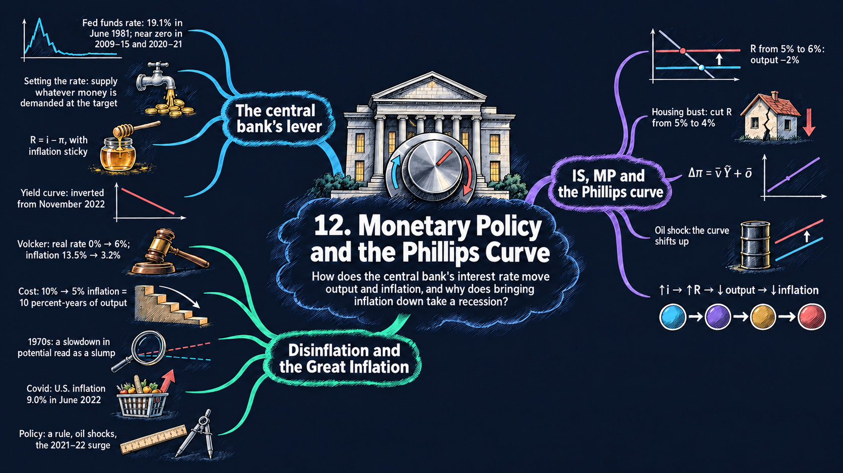




Learning goals
Chapter 11 built the IS curve, which links the real interest rate to short-run output. This chapter adds the two missing pieces of the short-run model: the MP curve (how the central bank sets the real interest rate) and the Phillips curve (how output moves inflation over time). By the end of it you will be able to:
- derive the MP curve from the Fisher equation and sticky inflation, and explain why a central bank that sets a nominal interest rate also sets the real rate in the short run;
- use the IS/MP diagram to analyze monetary policy and demand shocks, and derive the interest rate that keeps output at potential;
- derive the Phillips curve \(\Delta\pi_t = \bar{\nu}\tilde{Y}_t + \bar{o}\) from price setting with adaptive expectations and price shocks, and read its comparative statics;
- combine the IS, MP and Phillips curves into one equation for inflation, solve it for a disinflation and its cost in lost output, simulate the Volcker disinflation year by year, explain how mistakes contributed to the Great Inflation, and preview how an interest-rate rule (the Taylor rule) brings inflation back to target;
- read U.S. data on the federal funds rate, the yield curve, inflation and the Covid-19 recession, and compare them with dozens of other countries;
- in Python: draw several panels with
make_subplots, simulate a model with a loop, reshape tables withmeltandpivot, join tables withmerge, animate a chart withanimation_frame, and fit a trend withnp.polyfit.
Model overview
Islandia is back, and this time we watch it in the short run. In Chapter 11, Harbor Boatworks built fewer boats whenever borrowing got dearer, and Islandia’s output slipped below potential. That left two questions open: who sets the interest rate, and what does a boom or a slump do to Islandia’s prices? The Bank of Islandia answers the first, the Phillips curve the second, and together they complete the short-run model.
NoteThe big idea
The question. The Bank of Islandia controls only an overnight interest rate. How can that one lever move Islandia’s output this year and its inflation in the years after?
The answer in one sentence. Inflation is sticky, so the nominal rate the Bank sets also fixes the real rate (the MP curve), the real rate fixes short-run output (the IS curve), and output then nudges inflation up or down year after year (the Phillips curve).
What goes in and what comes out. We choose the path of the real interest rate, the demand shock \(\bar{a}\), the price shock \(\bar{o}\), the parameters \(\bar{b}\), \(\bar{r}\) and \(\bar{\nu}\), and the inflation of the year before we start. The model gives back short-run output and inflation in every year, and the nominal rate the Bank must set to get there.
Road map.
- The MP curve: why a nominal rate moves the real rate, and how short rates shape long ones.
- The IS/MP diagram: from the policy rate to output, and the rate that keeps output at potential.
- The Phillips curve: how a boom or a slump changes inflation.
- The full short-run model: the three equations together, a planned disinflation and its cost, and the dynamics after each kind of shock.
- An interest-rate rule: a first look at the Taylor rule of Chapter 13.
- Money demand and money supply: how the Bank makes its rate stick.
- Model in code: the key results as Python functions, checked with numbers. The drawing tools and the data helpers come after it.
Notation. A bar over a letter marks a parameter, a number taken from outside the model. Letters without a bar are endogenous variables; the real rate \(R_t\) is the Bank’s choice in most blocks, and a rule sets it in the Taylor block. Rates and inflation are in percent per year.
| Symbol | Meaning | Type |
|---|---|---|
| \(i_t\) | the nominal interest rate (the overnight policy rate) | endogenous |
| \(R_t\) | the real interest rate, chosen by the Bank (the MP curve) | endogenous |
| \(\pi_t\), \(\pi^e_t\) | inflation over the coming year, and the inflation firms expect | endogenous |
| \(\tilde{Y}_t\) | short-run output: the percentage gap between actual and potential output, \(> 0\) in a boom, \(< 0\) in a slump | endogenous |
| \(\bar{a}\) | aggregate demand shock (zero in normal times) | parameter |
| \(\bar{b}\) | how strongly spending reacts to the real rate | parameter |
| \(\bar{r}\) | the marginal product of capital | parameter |
| \(\bar{\nu}\), \(\bar{o}\) | the slope of the Phillips curve, and the price shock | parameters |
| \(\bar{m}\), \(\bar{\pi}\) | the rule’s response to inflation, and the inflation target (Taylor block) | parameters |
| \(M^d\), \(M^s\), \(m_0\) | money demanded, money supplied, and the position of money demand (last block) | notation |
| \(\Delta x_t\) | the change \(x_t - x_{t-1}\) of any variable from last year to this year | notation |
One baseline for every diagram. The textbook draws these diagrams without numbers, except in a few examples. Every figure and worked example of this notebook, and every number in Islandia’s story, starts from the same values:
- the IS curve of Chapter 11’s numerical example: no demand shock \(\bar{a} = 0\), \(\bar{b} = 2\) and a marginal product of capital \(\bar{r} = 5\) percent. Then the textbook’s “\(-2\) percent” in Figs. 4, 5 and 10 comes from \(R' = 6\) percent or from \(\bar{a}' = -2\);
- the slope of the Phillips curve \(\bar{\nu} = 0.5\) (illustrative; Chapter 9 estimated about 1/3 for the United States) and no price shock, \(\bar{o} = 0\);
- sticky inflation of 2 percent in normal times and 10 percent at the start of the Volcker disinflation (the textbook’s number);
- a money market with money demand \(M^d = 10 - i\) and money supply \(\bar{M}^s = 5\) (illustrative units), so that the nominal interest rate is 5 percent;
- for the productivity slowdown of Fig. 13, potential output growth of 3.5 percent a year before 1973 and 2.5 percent after (illustrative).
The MP curve: a nominal rate that moves the real rate
Assumptions
1. The policy instrument. The Bank of Islandia picks a short-term nominal interest rate \(i_t\): the rate at which Islandia’s banks lend to each other overnight. (In the United States this is the federal funds rate of Fig. 2.) The Bank makes its rate stick with a standing offer: it will lend, or borrow, any amount overnight at \(i_t\). No bank can then charge a borrower more than \(i_t\), because the borrower would simply go to the Bank. And no bank can lend for less for long. Other banks would borrow the cheap money and deposit it straight back at the Bank at \(i_t\), a riskless gain (an arbitrage), until the cheap lender had no funds left.
2. The Fisher equation of Chapter 8. A nominal interest rate covers two things: the real return \(R_t\), and the purchasing power that inflation \(\pi_t\) eats away,
\[i_t = R_t + \pi_t.\]
3. Sticky inflation. Islandia’s inflation has inertia. Over a short horizon, about six months, \(\pi_t\) does not respond to a policy move: when the Bank changes \(i_t\), it can treat \(\pi_t\) as given.
Solving the model
Step 1: the real interest rate. Take \(\pi_t\) away from both sides of the Fisher equation. The real rate is then the nominal rate minus inflation, equation (1) in the box below.
Step 2: what a policy move does. Compare Islandia just before and just after the Bank changes its rate. Write the real rate for both moments and subtract one from the other: \(\Delta R_t = \Delta i_t - \Delta\pi_t\). Inflation is sticky, so \(\Delta\pi_t = 0\) over that short horizon, and every point added to the nominal rate is a point added to the real rate.
ImportantKey result: the Bank of Islandia sets the real rate
\[R_t = i_t - \pi_t \tag{1}\]
\[\Delta R_t = \Delta i_t \qquad\text{(while inflation is sticky)}\]
So the Bank in effect chooses the real interest rate: for a target \(R^T\) it sets \(i_t = R^T + \pi_t\). In a diagram with short-run output \(\tilde{Y}\) on the horizontal axis and \(R\) on the vertical one, this choice is the MP curve. It does not depend on output, so it is a horizontal line at the chosen \(R_t\).
Islandia in numbers. With inflation at 2 percent, a nominal rate of 7 percent gives \(R = 5\% = \bar{r}\). With inflation at 10 percent, the same real rate needs a nominal rate of 15 percent, and 16 percent lifts the real rate to 6 percent.
TipIn words
What matters to Harbor Boatworks is what a loan costs in boats, not in money. Islandia’s prices only creep, so on the day the Bank adds a point to the money rate, prices have not moved, and the cost of a loan in goods rises by a full point. A central bank that sets only a money rate can therefore steer the real rate, for as long as inflation stays put.
Step 3: expected or actual inflation? A loan is signed before anyone knows how much prices will rise. So there are two real rates: the ex ante rate the borrower expects, \(R^{\text{ex ante}}_t = i_t - \pi^e_t\), and the ex post rate that is actually paid, \(R^{\text{ex post}}_t = i_t - \pi_t\). Subtract the first from the second:
\[R^{\text{ex post}}_t - R^{\text{ex ante}}_t = \pi^e_t - \pi_t.\]
Surprise inflation lowers the real rate actually paid: the borrower gains and the lender loses. Say Harbor Boatworks borrows at \(i = 7\) expecting inflation of 2, and inflation turns out to be 4 percent. It planned on a real rate of 5 percent but pays only 3. Investment plans rest on the ex ante rate; the short-run model ignores the gap and uses equation (1).
Step 4: from the overnight rate to long-term rates. Firms borrow for years, not for a night. Take an islander who saves for \(n\) years. One plan is a single \(n\)-year bond at the yearly rate \(i^{(n)}\). The other is a one-year bond now, then a fresh one-year bond each year, at the rates \(i_1, i^e_2, \dots, i^e_n\) expected today. If one plan paid more, nobody would choose the other, so in equilibrium the two pay the same:
\[(1 + i^{(n)})^n = (1 + i_1)(1 + i^e_2)\cdots(1 + i^e_n).\]
Now take logs of both sides (Appendix C.4). The log of a power is the exponent times the log, and the log of a product is the sum of the logs: \(n\ln(1+i^{(n)}) = \ln(1+i_1) + \ln(1+i^e_2) + \dots + \ln(1+i^e_n)\). For small rates, \(\ln(1+x) \approx x\) (Appendix C.6). Divide by \(n\):
\[i^{(n)} \approx \frac{i_1 + i^e_2 + \dots + i^e_n}{n}.\]
So a long-term rate is roughly the average of the short-term rates expected over its life. This link is the term structure of interest rates. If markets expect one-year rates of 2, 3, 4, 5 and 6 percent over the next five years, the five-year rate is close to 4 percent.
What the model predicts
| Change (inflation sticky unless stated) | Effect on \(R_t\) | In the IS/MP diagram |
|---|---|---|
| \(i_t\) up 1 point | \(+1\) point | the MP line shifts up |
| \(\pi_t\) up 1 point, \(i_t\) unchanged | \(-1\) point | the MP line shifts down |
| \(i_t\) and \(\pi_t\) both up 1 point | \(0\) | nothing moves |
| short rates expected to stay high for years | long rates rise toward them | (the yield curve shifts up) |
- Monetary policy has real effects only because inflation is sticky. If inflation jumped along with the nominal rate (the third row, the classical dichotomy), the real rate would stay where it was.
- A higher short rate today lifts long rates more when markets expect it to last. When the yield curve, the plot of interest rates against maturity, is inverted, markets expect short rates to fall (Fig. 6).
Because Islandia’s inflation is slow to move, the Bank of Islandia steers the real interest rate by setting a nominal one.
NoteCheck your understanding
1. Islandia’s inflation is 3 percent and the Bank wants a real rate of 5 percent. Which nominal rate must it set? A week later it raises that rate by half a point. What happens to the real rate?
Answer
By equation (1), \(i_t = R^T + \pi_t\), so the Bank sets 8 percent. Inflation is sticky over a week, so \(\Delta R_t = \Delta i_t\): the real rate rises by half a point too, to 5.5 percent.
2. Markets expect Islandia’s one-year rate to be 4 percent this year and 6 percent next year. About what is the two-year rate, and does the yield curve slope up or down?
Answer
By the term structure, the two-year rate is about the average of the expected one-year rates, \((4 + 6)/2 = 5\) percent. That is above today’s one-year rate, so the curve slopes up: markets expect short rates to rise.
The IS/MP diagram
Assumptions
1. The IS curve of Chapter 11. When borrowing costs more than a new tool earns, Harbor Boatworks and the islanders put off investment, and output falls below potential.
ImportantKey result: the IS curve (from Chapter 11)
\[\tilde{Y}_t = \bar{a} - \bar{b}\,(R_t - \bar{r}) \tag{2}\]
Short-run output falls when the real rate \(R_t\) rises above the marginal product of capital \(\bar{r}\). Here \(\bar{a}\) is the aggregate demand shock (zero in normal times), and \(\bar{b}\) measures how strongly investment demand reacts to the rate.
2. The MP curve. The Bank of Islandia sets \(R_t\), as we just derived.
Solving the model
Step 1: from the policy rate to output. Put equation (1) into equation (2):
\[\tilde{Y}_t = \bar{a} - \bar{b}\,(i_t - \pi_t - \bar{r}).\]
With \(\pi_t\) sticky, each extra point on the nominal rate costs \(\bar{b}\) percent of short-run output. Islandia sits where the MP line crosses the IS curve.
Step 2: the rate that delivers a target for output. Suppose the Bank wants output \(\tilde{Y}^T\). Set \(\tilde{Y}_t = \tilde{Y}^T\) in equation (2) and solve for \(R_t\). Move \(\tilde{Y}^T\) to the right and \(\bar{b}(R_t - \bar{r})\) to the left, \(\bar{b}(R_t - \bar{r}) = \bar{a} - \tilde{Y}^T\), then divide by \(\bar{b}\):
\[R_t = \bar{r} + \frac{\bar{a} - \tilde{Y}^T}{\bar{b}}.\]
The usual target is output at potential, \(\tilde{Y}^T = 0\).
ImportantKey result: the rate that keeps output at potential
\[R_t = \bar{r} + \frac{\bar{a}}{\bar{b}} \tag{3}\]
By equation (1), the nominal rate is then \(i_t = \bar{r} + \bar{a}/\bar{b} + \pi_t\). A fall in demand (\(\bar{a} < 0\)) is offset by cheaper credit, and each point of demand lost calls for a cut of \(1/\bar{b}\) points.
Islandia in numbers. With \(\bar{a} = 0\) and \(R = \bar{r} = 5\) percent, \(\tilde{Y} = 0\) (point \(A\) of Fig. 3). A real rate of 6 percent gives \(\tilde{Y} = -2 \times (6 - 5) = -2\) percent (Fig. 4). After a housing bust with \(\bar{a}' = -2\), output at \(R = 5\) is \(-2\) percent, and a cut to \(R' = 5 - 2/2 = 4\) percent brings it back to potential (Fig. 5).
TipIn words
Think of the IS curve as Harbor Boatworks’ order book. When the Bank raises the real rate, a new boat has to earn more to be worth its loan, so fewer are ordered and Islandia’s output slips below potential. When a housing bust drains demand, the Bank can cut the rate by just enough that cheaper credit fills the hole.
What the model predicts
| A rise of 1 in … | Effect on \(\tilde{Y}_t\) | Which curve moves |
|---|---|---|
| the real rate \(R_t\) | \(-\bar{b} = -2\) points | the MP line shifts up; the economy moves along the IS curve |
| the nominal rate \(i_t\) (inflation sticky) | \(-\bar{b} = -2\) points | the MP line shifts up |
| the demand shock \(\bar{a}\) | \(+1\) point | the IS curve shifts right |
| the marginal product of capital \(\bar{r}\) | \(+\bar{b} = +2\) points at a given \(R_t\) | the IS curve shifts up |
| the sensitivity \(\bar{b}\) | a larger effect of every rate change | the IS curve gets flatter |
- In the model, monetary policy can undo any demand shock completely: it only has to set \(R_t\) by equation (3).
- In practice this is hard. It takes time to learn how big a shock is, and a change in rates needs roughly 6 to 18 months to reach spending (Milton Friedman’s “long and variable lags”).
By choosing the real rate, the Bank of Islandia can in principle offset any demand shock and hold output at potential.
NoteCheck your understanding
1. A wave of optimism gives Islandia a demand shock \(\bar{a} = 1\). With \(\bar{b} = 2\) and \(\bar{r} = 5\) percent, which real rate keeps output at potential? With inflation at 2 percent, which nominal rate is that?
Answer
Equation (3) gives \(R = 5 + 1/2 = 5.5\) percent. By equation (1), the nominal rate is \(5.5 + 2 = 7.5\) percent. The Bank leans against the boom with a higher rate.
2. If equation (3) is so simple, why does the Bank of Islandia not keep output at potential all the time?
Answer
Because it must know \(\bar{a}\) when it sets the rate, and it does not. A shock is measured only with a delay, and a rate change takes many months to reach spending. By the time the cut works, the shock may have changed.
The Phillips curve
Assumptions
Inflation \(\pi_t \equiv (P_{t+1} - P_t)/P_t\) measures how much prices rise between this year and next. It is decided during year \(t\), when firms choose next year’s prices.
1. Price setting. Each firm on Islandia raises its prices by the inflation it expects elsewhere in the economy, \(\pi^e_t\), plus an adjustment for its own demand: a little more when orders are strong, a little less when they are weak. Adding up over all firms,
\[\pi_t = \pi^e_t + \bar{\nu}\tilde{Y}_t, \qquad \bar{\nu} > 0.\]
2. Adaptive expectations. Firms expect this year’s inflation to equal last year’s, \(\pi^e_t = \pi_{t-1}\). This is sticky inflation once more, now inside firms’ forecasts.
3. Price shocks. Now and then a shock \(\bar{o}\) adds to inflation directly. A jump in the price of fuel or steel, or a large union wage deal, gives \(\bar{o} > 0\); a wave of immigration that holds wages down gives \(\bar{o} < 0\). Most years, \(\bar{o} = 0\).
Solving the model
Step 1: the Phillips curve in levels. Replace \(\pi^e_t\) by \(\pi_{t-1}\) in the price-setting equation and add the price shock. This gives equation (4) below.
Step 2: in changes. Take \(\pi_{t-1}\) away from both sides of equation (4). This gives equation (5).
ImportantKey result: the Phillips curve
\[\pi_t = \pi_{t-1} + \bar{\nu}\tilde{Y}_t + \bar{o} \tag{4}\]
\[\Delta\pi_t = \bar{\nu}\tilde{Y}_t + \bar{o} \tag{5}\]
Short-run output does not set the level of inflation; it sets its change. A boom pushes inflation up, a slump pulls it down, and at potential (with no price shock) inflation stays where it was. The slope \(\bar{\nu}\) says how strongly prices react to demand.
Islandia in numbers. With \(\bar{\nu} = 0.5\), output 2 percent above potential raises inflation by \(0.5 \times 2 = 1\) point a year.
TipIn words
Every firm on Islandia starts from last year’s price rise and adds a little when its order book is full, or takes a little off when it is thin. So a boom does not raise inflation once and for all: it pushes inflation up another notch in every year it lasts. When output is back at potential the pushing stops, but inflation stays wherever it got to.
Step 3: inflation as a running total. Start from the inflation of the year before the first year, \(\pi_{-1}\), and apply equation (4) one year at a time (Appendix C.10):
\[\pi_0 = \pi_{-1} + \bar{\nu}\tilde{Y}_0 + \bar{o}_0, \qquad \pi_1 = \pi_0 + \bar{\nu}\tilde{Y}_1 + \bar{o}_1 = \pi_{-1} + \bar{\nu}(\tilde{Y}_0 + \tilde{Y}_1) + (\bar{o}_0 + \bar{o}_1).\]
Carry on for \(t + 1\) years, and each year adds one more output gap and one more price shock to the sums.
ImportantKey result: inflation adds up the past
\[\pi_t = \pi_{-1} + \bar{\nu}\sum_{s=0}^{t}\tilde{Y}_s + \sum_{s=0}^{t}\bar{o}_s \tag{6}\]
Inflation is the sum of all past output gaps and price shocks. Nothing is forgotten: once a gap has closed, inflation stays at its new level.
Step 4: when is inflation steady? Set \(\Delta\pi_t = 0\) in equation (5) and solve for output: \(\tilde{Y}_t = -\bar{o}/\bar{\nu}\). With no price shock, that is \(\tilde{Y}_t = 0\). After an oil shock of \(\bar{o} = 1\) point, steady inflation would take output of \(-1/0.5 = -2\) percent.
What the model predicts
| A rise of 1 in … | Effect on \(\Delta\pi_t\) | In the Phillips curve diagram |
|---|---|---|
| short-run output \(\tilde{Y}_t\) | \(+\bar{\nu} = +0.5\) point | a movement along the curve |
| the price shock \(\bar{o}\) | \(+1\) point at every \(\tilde{Y}_t\) | the curve shifts up for one period |
| the slope \(\bar{\nu}\) | a larger effect of every output gap | the curve gets steeper |
- Demand-pull and cost-push. The term \(\bar{\nu}\tilde{Y}_t\) is demand-pull inflation: strong demand pulls prices up. The shock \(\bar{o}\) is cost-push inflation: higher costs push them up.
- No lasting trade-off. Try to keep output above potential for ever, at \(\tilde{Y}_s = x > 0\). Equation (6) then gives \(\pi_t = \pi_{-1} + \bar{\nu}x(t+1)\), and inflation climbs without limit. A permanent boom cannot be bought with a higher but stable inflation rate, as the original Phillips curve of the 1960s seemed to promise. This is the argument of Milton Friedman and Edmund Phelps.
- Phillips curve and quantity theory. In the quantity theory of Chapter 8, faster growth of real GDP lowers inflation, while here a boom raises it. The two do not clash. The quantity theory speaks about the long run, where more output means more supply. Here a positive \(\tilde{Y}_t\) is demand beyond what the economy can normally supply.
Output sets the change in inflation, not its level, so a boom that never ends means inflation that never stops rising.
NoteCheck your understanding
1. Islandia’s inflation was 2 percent last year. This year output is 3 percent above potential, with no price shock and \(\bar{\nu} = 0.5\). What is inflation this year? If output is back at potential next year, what is inflation then?
Answer
Equation (4) gives \(\pi_t = 2 + 0.5 \times 3 = 3.5\) percent. Next year \(\tilde{Y} = 0\), so by equation (5) \(\Delta\pi = 0\): inflation stays at 3.5 percent. It does not go back to 2 on its own.
2. A smaller fuel-price shock, \(\bar{o} = 0.5\), hits Islandia. Which output gap would hold inflation steady that year, and which kind of inflation is the shock?
Answer
By step 4, \(\tilde{Y} = -\bar{o}/\bar{\nu} = -0.5/0.5 = -1\), a slump of 1 percent. The shock raises costs, so it is cost-push inflation.
The full short-run model: IS, MP and the Phillips curve together
Assumptions
Every year on Islandia, three things happen in turn: the Bank sets the rate, islanders and Harbor Boatworks decide how much to spend, and firms choose next year’s prices. Three equations hold:
| Block | Equation | Role |
|---|---|---|
| MP curve | the central bank chooses \(R_t\) (and sets \(i_t = R_t + \pi_t\)) | policy |
| IS curve | \(\tilde{Y}_t = \bar{a} - \bar{b}(R_t - \bar{r})\), equation (2) | \(R_t \Rightarrow \tilde{Y}_t\) |
| Phillips curve | \(\pi_t = \pi_{t-1} + \bar{\nu}\tilde{Y}_t + \bar{o}\), equation (4) | \(\tilde{Y}_t \Rightarrow \pi_t\) |
The model takes as given the path of policy \(R_t\), the shocks \(\bar{a}\) and \(\bar{o}\), the parameters \(\bar{b}\), \(\bar{r}\), \(\bar{\nu}\), and the inflation of the year before the first year, \(\pi_{-1}\). It determines short-run output \(\tilde{Y}_t\) and inflation \(\pi_t\) (and the nominal rate \(i_t\)) in every year. Within a year the chain runs one way only: \(R_t \Rightarrow \tilde{Y}_t \Rightarrow \pi_t\). Because \(\pi_t\) is the price rise over the coming year, a recession in year 0 already lowers year 0’s inflation: firms setting next year’s prices see this year’s weak demand.
Solving the model
Step 1: one equation for inflation. Replace \(\tilde{Y}_t\) in the Phillips curve (4) by the IS curve (2).
ImportantKey result: the whole model in one line
\[\pi_t = \pi_{t-1} + \bar{\nu}\left[\bar{a} - \bar{b}\,(R_t - \bar{r})\right] + \bar{o} \tag{7}\]
This is a difference equation: from last year’s inflation and this year’s policy and shocks, it gives this year’s inflation. Our simulate function below applies it year after year.
Step 2: a constant policy. Let the Bank hold \(R_t = R\) for some years, with \(\bar{a} = \bar{o} = 0\). Then \(\tilde{Y}_t = -\bar{b}(R - \bar{r})\) is the same in every year, and equation (6) gives \(\pi_t = \pi_{-1} + (t+1)\,\bar{\nu}\tilde{Y} = \pi_{-1} - (t+1)\,\bar{\nu}\bar{b}(R - \bar{r})\). Inflation falls by the same \(\bar{\nu}\bar{b}(R - \bar{r})\) points each year: a straight line.
Step 3: designing a disinflation. The Bank wants inflation to go from \(\pi_{-1}\) to a target \(\pi^T\) in \(T\) years, with a constant real rate. After \(T\) years (in year \(T - 1\)), step 2 says \(\pi^T = \pi_{-1} + T\bar{\nu}\tilde{Y}\). Solve for the output gap, \(\tilde{Y} = -(\pi_{-1} - \pi^T)/(\bar{\nu}T)\), and then solve the IS curve for the rate that delivers it, \(R - \bar{r} = -\tilde{Y}/\bar{b}\). That rate is equation (8) below.
Step 4: the cost. The output lost is the sum of the gaps, \(\sum_{t=0}^{T-1}(-\tilde{Y}) = T \times (\pi_{-1} - \pi^T)/(\bar{\nu}T)\). The \(T\) cancels, which gives equation (9).
ImportantKey result: the recipe and the price of a disinflation
\[R = \bar{r} + \frac{\pi_{-1} - \pi^T}{\bar{\nu}\bar{b}\,T} \tag{8}\]
\[\text{lost output} = \frac{\pi_{-1} - \pi^T}{\bar{\nu}} \quad\text{percent-years} \tag{9}\]
Equation (6) with no price shocks says that any output path with \(\sum_s \tilde{Y}_s = (\pi^T - \pi_{-1})/\bar{\nu}\) does the job. So equation (9) holds whatever the shape of the recession: each point of inflation removed costs \(1/\bar{\nu}\) percent-years of output.
Islandia in numbers. From \(\pi_{-1} = 10\) to \(\pi^T = 5\) percent in \(T = 5\) years, with \(\bar{\nu} = 0.5\), \(\bar{b} = 2\) and \(\bar{r} = 5\): equation (8) gives \(R = 5 + 5/(0.5 \times 2 \times 5) = 6\) percent, so \(\tilde{Y} = -2\) percent every year, and inflation runs 9, 8, 7, 6, 5. Equation (9) puts the cost at \(5/0.5 = 10\) percent-years. This is Fig. 12.
TipIn words: the price of disinflation
Lowering Islandia’s inflation has a fixed price, paid in lost output. The Bank can pay it fast, with a short and deep recession, or slowly, with a long and shallow one, but the bill is the same. Only a steeper Phillips curve, prices that react more to slack, makes it cheaper.
Step 5: where inflation comes to rest. Once policy is back at \(R_t = \bar{r} + \bar{a}/\bar{b}\) (equation 3), output is at potential and, with \(\bar{o} = 0\), \(\Delta\pi_t = 0\): inflation stays at whatever level it has reached. Any inflation rate can be a resting point. Nothing in the model pulls inflation back toward a particular level; only policy can move it.
NoteCheck your understanding
1. Islandia’s inflation is 8 percent, and the Bank wants 4 percent in two years (\(\bar{\nu} = 0.5\), \(\bar{b} = 2\), \(\bar{r} = 5\)). Which real rate should it hold, and how much output does the plan cost?
Answer
Equation (8) gives \(R = 5 + 4/(0.5 \times 2 \times 2) = 7\) percent, so \(\tilde{Y} = -2 \times (7 - 5) = -4\) percent in each of the two years. Equation (9) puts the cost at \(4/0.5 = 8\) percent-years, the same as a slower plan would cost.
What the model predicts
The dynamics after each kind of event, with the baseline \(\bar{b} = 2\), \(\bar{\nu} = 0.5\) and \(R_t = \bar{r}\) unless stated:
| Event | Output | Inflation |
|---|---|---|
| tight policy, \(R = \bar{r} + 1\) for \(T\) years | \(\tilde{Y} = -2\) while it lasts | falls 1 point a year, then stays at the lower level |
| demand boom \(\bar{a} = 2\) for \(T\) years, \(R\) unchanged | \(\tilde{Y} = +2\) while it lasts | rises 1 point a year, then stays higher |
| the same boom, policy follows equation (3) | \(\tilde{Y} = 0\) | unchanged |
| a one-year price shock \(\bar{o} = 1\) | \(\tilde{Y} = 0\) | up 1 point, and stays up |
| the same shock, then the central bank undoes it | a recession of \(\bar{o}/\bar{\nu} = 2\) percent-years in total | back to where it started |
| a slowdown in potential mistaken for \(\bar{a}' = -2\) | \(\tilde{Y} = -\bar{a}' = +2\) | rises 1 point a year |
The last row is the policy mistake of the 1970s (Figs. 13 and 21). The policymakers cut the rate by equation (3) to \(R' = \bar{r} + \bar{a}'/\bar{b}\). But the true IS curve still has \(\bar{a} = 0\), so true output is \(\tilde{Y} = -\bar{b}(R' - \bar{r}) = -\bar{b}\,\bar{a}'/\bar{b} = -\bar{a}'\): a boom, not a return to potential.
- With sticky inflation and adaptive expectations, the only way to bring inflation down is a spell of output below potential (equation 9). Disinflation is a temporary recession, not a permanent loss.
- Inflation keeps a memory of every shock (equation 6). Oil shocks, too-loose policy and a misread productivity slowdown can therefore pile up into a Great Inflation.
Inflation remembers every shock, and the only way to bring it down is a spell of output below potential.
NoteCheck your understanding
1. The Bank of Islandia thinks demand has fallen, \(\bar{a}' = -1\), but in truth potential output has slowed and \(\bar{a} = 0\). Which rate does it set by equation (3), and what happens to output and inflation?
Answer
It cuts to \(R' = 5 - 1/2 = 4.5\) percent. The true IS curve (2) gives \(\tilde{Y} = -2 \times (4.5 - 5) = +1\) percent: a boom. By equation (5), inflation then rises by \(0.5 \times 1 = 0.5\) points a year for as long as the mistake lasts.
Looking ahead: an interest-rate rule (the Taylor rule)
Assumptions
Up to now the Bank of Islandia sets each year’s real rate by judgment. Chapter 13 has it follow a rule instead: for every point that inflation sits above an inflation target \(\bar{\pi}\), the real rate goes \(\bar{m}\) points above \(\bar{r}\),
\[R_t - \bar{r} = \bar{m}\,(\pi_t - \bar{\pi}), \qquad \bar{m} > 0.\]
By the Fisher equation, the nominal rate is then \(i_t = R_t + \pi_t = \bar{r} + \pi_t + \bar{m}(\pi_t - \bar{\pi})\). This is the inflation part of the Taylor rule; John Taylor’s full rule also reacts to short-run output. The IS curve (2) and the Phillips curve (4) are unchanged. Here we only preview the result, with this chapter’s numbers.
Solving the model
Step 1: the rule in the IS curve. Replace \(R_t - \bar{r}\) in equation (2): \(\tilde{Y}_t = \bar{a} - \bar{b}\bar{m}(\pi_t - \bar{\pi})\). Higher inflation now brings a higher real rate and lower output. Chapter 13 calls this the AD curve.
Step 2: into the Phillips curve. Put it into equation (4) and subtract \(\bar{\pi}\) from both sides. With the inflation gap \(x_t \equiv \pi_t - \bar{\pi}\),
\[x_t = x_{t-1} + \bar{\nu}\bar{a} - \bar{\nu}\bar{b}\bar{m}\,x_t + \bar{o}.\]
The gap \(x_t\) shows up on both sides, because this year’s inflation sets this year’s rate. Gather the \(x_t\) terms on the left, \((1 + \bar{\nu}\bar{b}\bar{m})\,x_t = x_{t-1} + \bar{\nu}\bar{a} + \bar{o}\), and divide by \(1 + \bar{\nu}\bar{b}\bar{m}\). Call the result’s factor \(\lambda \equiv 1/(1 + \bar{\nu}\bar{b}\bar{m})\): this is equation (10) in the box below.
Step 3: the path with no shocks. With \(\bar{a} = \bar{o} = 0\), the gap obeys \(x_t = \lambda x_{t-1}\), so \(x_0 = \lambda x_{-1}\), \(x_1 = \lambda^2 x_{-1}\), and so on, one more factor \(\lambda\) each year.
ImportantKey result: inflation under the rule
\[\pi_t - \bar{\pi} = \lambda\left[(\pi_{t-1} - \bar{\pi}) + \bar{\nu}\bar{a} + \bar{o}\right], \qquad \lambda \equiv \frac{1}{1 + \bar{\nu}\bar{b}\bar{m}} \tag{10}\]
\[\pi_t - \bar{\pi} = \lambda^{t+1}\,(\pi_{-1} - \bar{\pi}) \tag{11}\]
Since \(0 < \lambda < 1\), the gap shrinks by the same fraction every year, and inflation returns to the target by itself (Appendix C.10). Output follows the gap, \(\tilde{Y}_t = -\bar{b}\bar{m}\,x_t\).
Islandia in numbers. With \(\bar{\nu} = 0.5\), \(\bar{b} = 2\), Taylor’s \(\bar{m} = 1/2\) and a target of 2 percent, \(\bar{\nu}\bar{b}\bar{m} = 0.5\) and \(\lambda = 1/1.5 = 2/3\). From 10 percent inflation, the gap of 8 points becomes \(5.33\), \(3.56\), \(2.37\), …: inflation runs about \(7.3\), \(5.6\), \(4.4\) percent, and output \(-5.3\), \(-3.6\), \(-2.4\) percent. The total output lost is \(8 \times (2/3)/(1 - 2/3) = 16\) percent-years, exactly \((\pi_{-1} - \bar{\pi})/\bar{\nu} = 8/0.5\), as equation (9) requires.
TipIn words
Under the rule, the Bank of Islandia leans harder the further inflation is from its target. High inflation brings a high real rate, a slump, and so falling inflation; as inflation nears the target, the Bank eases off. Each year the same share of the remaining gap disappears, so the return is fast at first and gentle at the end.
What the model predicts
- Each year Islandia closes the share \(1 - \lambda = \bar{\nu}\bar{b}\bar{m}/(1 + \bar{\nu}\bar{b}\bar{m})\) of its inflation gap: one third at the baseline. A tougher Bank (larger \(\bar{m}\)), more rate-sensitive spending (larger \(\bar{b}\)) or a steeper Phillips curve (larger \(\bar{\nu}\)) all make \(\lambda\) smaller and the return faster.
- A tougher rule front-loads the recession but does not make it cheaper. By equation (6), the total output lost is still \((\pi_{-1} - \bar{\pi})/\bar{\nu}\), whatever \(\bar{m}\).
- The nominal rate rises by \(1 + \bar{m}\) points for each point of inflation, more than one for one, so that the real rate goes up. This is the Taylor principle.
A rule that raises the real rate when inflation is high brings inflation back to target on its own, but never for free.
NoteCheck your understanding
1. The Bank of Islandia becomes tougher, \(\bar{m} = 1\), with \(\bar{\nu} = 0.5\) and \(\bar{b} = 2\). Starting from 10 percent inflation and a target of 2 percent, what is \(\lambda\), what is inflation in year 0, and how much output is lost in total?
Answer
Now \(\bar{\nu}\bar{b}\bar{m} = 1\), so \(\lambda = 1/2\). Equation (11) gives \(\pi_0 = 2 + 0.5 \times 8 = 6\) percent, a faster fall than the 7.3 percent with \(\bar{m} = 1/2\). The total cost is unchanged, \(8/0.5 = 16\) percent-years: the recession is deeper but shorter.
Microfoundations: money demand, money supply and the policy rate
Assumptions
1. Money demand. Cash and checking accounts pay no interest, while a savings account pays \(i\). Holding money therefore means giving up \(i\): the nominal rate is the opportunity cost of money, and islanders keep less of it when the rate is high. We use an illustrative straight line, \(M^d = m_0 - i\), with \(m_0 = 10\) at the baseline. Higher prices or output, or new ways of paying, shift \(m_0\).
2. Money supply. The Bank of Islandia decides how much money to supply, \(M^s\): a vertical line in a diagram with money on the horizontal axis and \(i\) on the vertical one.
3. Sticky inflation. In the short run the price level does not jump to clear the money market, as it would in the quantity theory. The interest rate does the clearing instead (and with it, the velocity of money).
Solving the model
Step 1: the equilibrium rate. Set money demand equal to money supply, \(m_0 - i^* = M^s\), and solve for \(i^*\).
ImportantKey result: the rate that clears the money market
\[i^* = m_0 - M^s \tag{12}\]
Above \(i^*\), islanders want to hold less money than there is, and the rate falls; below it, they want more, and the rate rises.
Islandia in numbers. At the baseline, \(i^* = 10 - 5 = 5\) percent.
Step 2: comparative statics. By equation (12), one unit less money supply raises \(i^*\) by one point, and one unit more money demand does the same. Cutting the supply from 5 to 4 units lifts the rate from 5 to 6 percent: tight money means a higher interest rate (Fig. 19).
Step 3: targeting the rate. To hold the rate at a target \(i^T\) whatever happens to demand, solve equation (12) for the supply: \(M^s = m_0 - i^T\). Supply now moves one for one with demand, and the rate does not move at all. In the diagram, money supply becomes a horizontal line at \(i^T\). If demand rises to \(m_0 = 11\), the Bank supplies 6 units instead of 5 (Fig. 20).
TipIn words
The Bank of Islandia stands ready to swap money for bonds at its chosen rate. When islanders want more cash, it simply supplies more; when they want less, it takes some back. The quantity of money adjusts in the background, and the rate, the thing that matters for spending, stays put.
Step 4: bonds and open-market operations. The Bank changes the money supply by buying or selling government bonds. A bond that pays 100 dollars in a year and costs \(P_B\) today earns \(100 - P_B\) on an outlay of \(P_B\), so its interest rate is
\[i = \frac{100 - P_B}{P_B} \quad\Longleftrightarrow\quad P_B = \frac{100}{1 + i}.\]
A bond priced at 96 dollars yields \(4/96 \approx 4.2\) percent. When the Bank sells bonds, it takes money out of the economy and pushes bond prices down, so the interest rate rises; buying bonds does the opposite.
What the model predicts
| Change | Effect on \(i^*\) with \(M^s\) fixed | Effect when the central bank targets \(i\) |
|---|---|---|
| money supply down 1 unit | \(+1\) point | (not used: \(M^s\) follows demand) |
| money demand \(m_0\) up 1 unit | \(+1\) point | \(0\); \(M^s\) rises by 1 unit |
- With a fixed money supply, every swing in money demand would move the interest rate, and with sticky inflation also the real rate and output, though nothing real had happened. Targeting the rate shields the economy from such shocks. That is why modern central banks set an interest rate rather than a quantity of money.
- IS/LM. Hold \(M^s\) fixed and let higher output raise money demand: the rate then rises with output, an upward-sloping “LM” curve. A central bank that adjusts \(M^s\) to hold its rate turns that curve into our flat MP line.
The Bank of Islandia makes its rate stick by supplying whatever money islanders want at that rate.
NoteCheck your understanding
1. Islanders’ money demand rises to \(M^d = 12 - i\). If the Bank keeps the supply at 5 units, what is the rate? Which supply would keep the rate at 5 percent?
Answer
Equation (12) gives \(i^* = 12 - 5 = 7\) percent. To hold 5 percent, the Bank solves \(M^s = m_0 - i^T = 12 - 5\), so it supplies 7 units.
2. A one-year bond that pays 100 dollars sells for 98 dollars. What is its interest rate? If the Bank sells bonds and the price falls, does the rate rise or fall?
Answer
The rate is \(2/98 \approx 2.04\) percent, from \(i = (100 - P_B)/P_B\). A lower price means a larger gain per dollar spent, so the rate rises.
NoteRecap
- The MP curve: with sticky inflation, the Bank of Islandia’s nominal rate sets the real rate, \(R_t = i_t - \pi_t\) (Fig. 3).
- The IS/MP diagram: each point on the real rate lowers output by \(\bar{b}\), and equation (3) keeps output at potential after a demand shock (Fig. 5).
- The Phillips curve: output sets the change in inflation, \(\Delta\pi_t = \bar{\nu}\tilde{Y}_t + \bar{o}\) (Fig. 7, Fig. 8).
- Disinflation has a fixed price: \((\pi_{-1} - \pi^T)/\bar{\nu}\) percent-years of output, however the recession is spread (Fig. 12).
- A rule closes the gap step by step: under the Taylor rule, the inflation gap shrinks by the factor \(\lambda\) each year.
- The Bank makes its rate stick by standing ready to supply any amount of money islanders want at its rate (Fig. 20).
Model in code
Now we turn the Key results into Python. The section has four parts: the setup (folded, because it is the same in every chapter), the model as functions, numerical checks of the Key results, and the drawing and data tools that the figures use (folded too). Run its cells once, in order. Every later section of the notebook reuses them.
Setup
Run the setup cells once, before anything else. They load the Python libraries, give every chart the same look, store the address of the chapter’s data and define a helper that only the book website needs. You can use the notebook without reading them; open the box if you are curious.
NoteShow the setup code
The first cell loads the libraries and sets the look of the charts. Its comments explain each step.
The website cannot run Python, so each interactive figure also gets a version with a precomputed slider. The next helper builds those versions. Run it and move on.
# @title Helper for the website versions (run this cell; you do not need to read it)
def slider_figure(make_figure, name, values, start, label=None):
    """Join precomputed versions of a figure with one slider (the website cannot run Python).

    Arguments
        make_figure : the function that draws the figure, e.g. a diagram of this chapter
        name        : the argument the slider moves, e.g. "nu"
        values      : the values of that argument to precompute
        start       : the value shown first
        label       : the slider's label (the argument name if None)
    Returns
        one Plotly figure with all versions and a slider that shows one at a time
    """
    # Step 1: draw the figure once for every value
    figures = [make_figure(**{name: v}) for v in values]
    first = values.index(start)
    # Step 2: copy every curve into one figure; only the start value's are visible
    fig = go.Figure(layout=figures[first].layout)
    owner = []                          # which precomputed figure each trace is from
    for i, f in enumerate(figures):
        for trace in f.data:
            trace.visible = (i == first)
            fig.add_trace(trace)
            owner.append(i)
    # Step 3: one slider step per value: its curves, title, labels and shapes
    steps = []
    for i, f in enumerate(figures):
        layout = {"title": f.layout.title.to_plotly_json(),
                  "annotations": [a.to_plotly_json() for a in f.layout.annotations],
                  "shapes": [s.to_plotly_json() for s in f.layout.shapes]}
        visible = [o == i for o in owner]
        steps.append(dict(method="update", label=str(values[i]), args=[{"visible": visible}, layout]))
    fig.update_layout(sliders=[dict(active=first, steps=steps, pad=dict(t=60),
                                    currentvalue=dict(prefix=(label or name) + " = "))])
    return fig
The model as functions
The short-run model rests on four Key results: the Fisher equation (1), the IS curve (2) and the rate that gives a chosen output (3), and the Phillips curve (5). We write each one as a Python function: a named recipe that takes inputs and gives back a result. The first cell also stores the parameters of the chapter’s examples, which the functions use as default values.
# The parameters of the model, used below as default values.
# IS curve: no demand shock, b-bar = 2, r-bar = 5 percent
A_BAR, B_BAR, R_BAR = 0.0, 2.0, 5.0
# Phillips curve: slope nu-bar = 0.5, no price shock
NU, O_BAR = 0.5, 0.0
# money market: demand M = 10 - i, supply 5 (units)
M0, M_BAR = 10.0, 5.0


# `def` creates a function. Its inputs are the arguments in parentheses.
# The text in triple quotes describes the function.
def real_rate(i, pi):
    """The real interest rate, from the Fisher equation.

    Equation (1):  R = i - pi

    Arguments
        i  : the nominal interest rate, in percent
        pi : inflation, in percent
    Returns
        the real interest rate R, in percent
    """
    # `return` gives back the result
    return i - pi


# `b=B_BAR` gives b a default value, used whenever we do not pass one; here the
# default is a constant we defined just above
def is_curve(R, a=A_BAR, b=B_BAR, r_bar=R_BAR):
    """Short-run output, from the IS curve.

    Equation (2):  Y~ = a - b (R - r_bar)

    Arguments
        R     : the real interest rate, in percent
        a     : the demand shock, a-bar (0 unless we pass another value)
        b     : how strongly output reacts to the real rate, b-bar
        r_bar : the marginal product of capital, r-bar, in percent
    Returns
        short-run output Y~, in percent of potential output
    """
    # each point of R above r-bar lowers output by b points
    return a - b * (R - r_bar)


def rate_for_output(Y, a=A_BAR, b=B_BAR, r_bar=R_BAR):
    """The real interest rate at which short-run output equals Y: the IS curve solved for R.

    Equation (3) when Y = 0:  R = r_bar + (a - Y) / b

    Arguments
        Y           : the short-run output we want, Y~, in percent
        a, b, r_bar : the parameters of the IS curve, as in is_curve
    Returns
        the real interest rate R, in percent
    """
    # equation (2), Y = a - b (R - r_bar), solved for R
    return r_bar + (a - Y) / b


def phillips(Y, nu=NU, o=O_BAR):
    """The change in inflation, from the Phillips curve.

    Equation (5):  change in inflation = nu Y~ + o

    Arguments
        Y  : short-run output, Y~, in percent
        nu : the slope of the Phillips curve, nu-bar
        o  : the price shock, o-bar (0 unless we pass another value)
    Returns
        the change in inflation, in percentage points
    """
    # a boom (Y > 0) raises inflation, a slump lowers it, a price shock adds o
    return nu * Y + o
The money market has two more functions. People hold less money when the nominal interest rate, the opportunity cost of holding money, is higher. The rate that clears the market is where money demand equals the supply.
def money_demand(i, m0=M0):
    """Money demanded at the nominal interest rate i, the demand curve of Fig. 18.

    Money demand:  M = m0 - i

    Arguments
        i  : the nominal interest rate, in percent
        m0 : money demanded at a zero interest rate (10 in the chapter's examples)
    Returns
        the amount of money demanded, M
    """
    # one point more on i, one unit less money held
    return m0 - i


def market_rate(M_s, m0=M0):
    """The nominal interest rate that clears the money market.

    Equation (12):  money demand m0 - i equals the supply M_s, so i = m0 - M_s

    Arguments
        M_s : the money supply, set by the central bank
        m0  : money demanded at a zero interest rate
    Returns
        the equilibrium nominal interest rate i, in percent
    """
    return m0 - M_s
The full model runs year by year: the central bank sets \(R_t\), the IS curve gives \(\tilde{Y}_t\), and the Phillips curve turns last year’s inflation into this year’s. simulate repeats these three steps for a whole path of interest rates.
def simulate(R_path, pi_start, nu=NU, a=A_BAR):
    """The short-run model year by year: MP sets R, IS gives Y~, the Phillips curve gives pi.

    Equation (7), one year at a time:  pi_t = pi_(t-1) + nu (a - b (R_t - r_bar))

    Arguments
        R_path   : the real interest rate of each year, a list, in percent
        pi_start : inflation in the year before the first year, in percent
        nu       : the slope of the Phillips curve, nu-bar
        a        : the demand shock, a-bar
    Returns
        two arrays: short-run output Y~ and inflation pi in each year
    """
    # Step 1: two empty lists; `.append(...)` adds one number at the end of a list
    Y_path, pi_path = [], []
    pi = pi_start                          # inflation of the year before the first year
    # Step 2: a `for` loop runs the indented lines once for each rate in `R_path`
    for R in R_path:
        Y = is_curve(R, a)                 # the IS curve gives this year's output
        pi = pi + phillips(Y, nu)          # last year's inflation, adjusted for demand
        Y_path.append(Y)
        pi_path.append(pi)
    # Step 3: `np.array(...)` turns a list into an array, for arithmetic with it
    return np.array(Y_path), np.array(pi_path)
Checking the key results
The functions came from algebra. Now we check them with numbers. First we try them on the textbook’s examples: the Fisher equation, the IS curve, a housing bust, a slump and an oil shock in the Phillips curve, the money market, and the Volcker disinflation.
# The textbook's examples, one line each.
# An f-string, f"R = {value:.1f}%", puts a value into the text; ":.1f" means
# "one decimal" and ":+.2f" "the sign and two decimals".
print(f"Fisher: i = 7%, pi = 2%    ->  R = {real_rate(7.0, 2.0):.1f}%")
print(f"IS: R = 5%  ->  Y~ = {is_curve(5.0):+.1f}%;   R = 6%  ->  Y~ = {is_curve(6.0):+.1f}%")
print(f"Housing bust a' = -2: the rate that keeps Y~ = 0 is R' = {rate_for_output(0.0, a=-2.0):.1f}%")
print(f"Phillips curve: Y~ = -2%  ->  change in inflation {phillips(-2.0):+.2f} points")
print(f"Oil shock o = 1 at Y~ = 0  ->  change in inflation {phillips(0.0, o=1.0):+.2f} points")
print(f"Money market: supply 5  ->  i = {market_rate(5.0):.1f}%;   supply 4  ->  i = {market_rate(4.0):.1f}%")
# the Volcker disinflation: five years at R = 6%, then back to r-bar = 5%
Y_path, pi_path = simulate([6.0, 6.0, 6.0, 6.0, 6.0, 5.0], pi_start=10.0)
print("Volcker: five years at R = 6%, then R = 5%. Inflation:", pi_path)
Fisher: i = 7%, pi = 2% -> R = 5.0%
IS: R = 5% -> Y~ = +0.0%; R = 6% -> Y~ = -2.0%
Housing bust a' = -2: the rate that keeps Y~ = 0 is R' = 4.0%
Phillips curve: Y~ = -2% -> change in inflation -1.00 points
Oil shock o = 1 at Y~ = 0 -> change in inflation +1.00 points
Money market: supply 5 -> i = 5.0%; supply 4 -> i = 6.0%
Volcker: five years at R = 6%, then R = 5%. Inflation: [9. 8. 7. 6. 5. 5.]Raising the real interest rate from 5 to 6 percent pushes output 2 percent below potential. With \(\bar{\nu} = 0.5\), a 2 percent recession lowers inflation by 1 point a year, so five years of it bring inflation from 10 down to 5 percent, and it stays there once the interest rate is back at \(\bar{r}\).
Check 1: the MP curve and equation (3). With inflation sticky, a point on \(i\) must move \(R\) by a point; if inflation rises with \(i\), \(R\) must not move. Equation (3) must give a rate at which the IS curve returns exactly \(\tilde{Y} = 0\), and the slope of the IS curve must be \(-\bar{b}\).
# Step 1: the MP curve, equation (1), with sticky and with moving inflation
R_before = real_rate(7.0, 2.0)
print(f"i 7% -> 8%, pi sticky at 2%:   R changes by {real_rate(8.0, 2.0) - R_before:+.1f} point")
print(f"i 7% -> 8% and pi 2% -> 3%:    R changes by {real_rate(8.0, 3.0) - R_before:+.1f} points")
# Step 2: for three demand shocks a, the rate of equation (3) must give Y~ = 0
for a in [-2.0, -1.0, 1.5]:
    R_stab = R_BAR + a / B_BAR                                   # equation (3)
    print(f"a = {a:+.1f}: equation (3) gives R = {R_stab:.2f}%, and there the IS curve gives Y~ = {is_curve(R_stab, a=a):+.2f}%")
# Step 3: the slope of the IS curve, from two rates one point apart
print(f"Slope of the IS curve: {is_curve(6.0) - is_curve(5.0):+.1f} points of output per point of R (-b = {-B_BAR:.1f})")
i 7% -> 8%, pi sticky at 2%: R changes by +1.0 point
i 7% -> 8% and pi 2% -> 3%: R changes by +0.0 points
a = -2.0: equation (3) gives R = 4.00%, and there the IS curve gives Y~ = +0.00%
a = -1.0: equation (3) gives R = 4.50%, and there the IS curve gives Y~ = +0.00%
a = +1.5: equation (3) gives R = 5.75%, and there the IS curve gives Y~ = +0.00%
Slope of the IS curve: -2.0 points of output per point of R (-b = -2.0)Check 2: the term structure. The five-year rate that matches five one-year bonds in a row, computed exactly, should be close to the simple average of the expected one-year rates.
# Step 1: the expected one-year rates over the next five years, in percent
expected = [2.0, 3.0, 4.0, 5.0, 6.0]
# Step 2: roll the money over, one year at a time: each time round the loop,
# `growth` is multiplied by one more factor (1 + rate)
growth = 1.0
for rate in expected:
    growth = growth * (1 + rate / 100)
# Step 3: `**` means "to the power of", so `** (1 / 5)` takes the fifth root;
# `np.mean` is the average of a list
exact = 100 * (growth ** (1 / 5) - 1)
print(f"Five-year rate, exact:          {exact:.3f}%")
print(f"Average of the one-year rates:  {np.mean(expected):.3f}%")
Five-year rate, exact: 3.990%
Average of the one-year rates: 4.000%Check 3: the disinflation, equations (6), (8) and (9). We let equation (8) choose the real rate that takes inflation from 10 to 5 percent in five years, run simulate, and compare each year’s inflation with the running total of equation (6) and the total cost with equation (9).
# Step 1: from 10 to 5 percent inflation in T = 5 years; equation (8) gives the rate
pi_start, pi_target, T = 10.0, 5.0, 5
R_high = R_BAR + (pi_start - pi_target) / (NU * B_BAR * T)      # equation (8)
# Step 2: R_high for T years, then r-bar for two years. `[R_high] * T` is a list
# with T copies of R_high, and `+` joins two lists.
Y_path, pi_path = simulate([R_high] * T + [R_BAR, R_BAR], pi_start)
print(f"Equation (8): hold R at {R_high:.2f}% for {T} years")
# Step 3: each year, the running total of equation (6), with no price shocks.
# `Y_path[: t + 1]` keeps the first t + 1 numbers of the array (years 0 to t),
# and `.sum()` adds them up.
for t in range(T + 2):
    total = pi_start + NU * Y_path[: t + 1].sum()
    print(f"Year {t}: Y~ = {Y_path[t]:+.1f}%, pi = {pi_path[t]:.2f}% (simulated), {total:.2f}% (equation 6)")
# Step 4: the total output lost, against equation (9)
print(f"Output lost: {-Y_path.sum():.1f} percent-years;  equation (9): {(pi_start - pi_target) / NU:.1f}")
# Step 5: a faster disinflation, from 10 to 4 percent in four years
R_fast = R_BAR + (10.0 - 4.0) / (NU * B_BAR * 4)
print(f"From 10% to 4% in 4 years: R = {R_fast:.2f}%, inflation path {simulate([R_fast] * 4, 10.0)[1]}")
Equation (8): hold R at 6.00% for 5 years
Year 0: Y~ = -2.0%, pi = 9.00% (simulated), 9.00% (equation 6)
Year 1: Y~ = -2.0%, pi = 8.00% (simulated), 8.00% (equation 6)
Year 2: Y~ = -2.0%, pi = 7.00% (simulated), 7.00% (equation 6)
Year 3: Y~ = -2.0%, pi = 6.00% (simulated), 6.00% (equation 6)
Year 4: Y~ = -2.0%, pi = 5.00% (simulated), 5.00% (equation 6)
Year 5: Y~ = +0.0%, pi = 5.00% (simulated), 5.00% (equation 6)
Year 6: Y~ = +0.0%, pi = 5.00% (simulated), 5.00% (equation 6)
Output lost: 10.0 percent-years; equation (9): 10.0
From 10% to 4% in 4 years: R = 6.50%, inflation path [8.5 7. 5.5 4. ]Check 4: shocks with an unchanged interest rate. A one-year price shock should raise inflation for good when the real rate stays at \(\bar{r}\). And a cut by equation (3) for a demand shock that never happened should give true output \(\tilde{Y} = -\bar{a}'\).
# Step 1: a price shock o = 1 in the first year only, with R held at r-bar
pi = 2.0
for o in [1.0, 0.0, 0.0, 0.0]:
    pi = pi + phillips(is_curve(R_BAR), o=o)     # equation (4) with R = r-bar
    print(f"Price shock {o:.1f}: inflation {pi:.1f}%")
# Step 2: undoing it costs 1/nu percent-years of output; `[1]` picks the second
# result of `simulate`, the path of inflation
print(f"Undoing it costs {1.0 / NU:.1f} percent-years of output:", simulate([R_BAR + 1.0, R_BAR], 3.0)[1])
# Step 3: the Bank believes the IS curve shifted by a', and cuts R by equation (3)
for a_believed in [-2.0, -1.0]:
    R_cut = rate_for_output(0.0, a=a_believed)
    print(f"Believed a' = {a_believed:+.1f}: R cut to {R_cut:.2f}%, true Y~ = {is_curve(R_cut):+.1f}%")
Price shock 1.0: inflation 3.0%
Price shock 0.0: inflation 3.0%
Price shock 0.0: inflation 3.0%
Price shock 0.0: inflation 3.0%
Undoing it costs 2.0 percent-years of output: [2. 2.]
Believed a' = -2.0: R cut to 4.00%, true Y~ = +2.0%
Believed a' = -1.0: R cut to 4.50%, true Y~ = +1.0%Check 5: the interest-rate rule, equations (10) and (11). Each year we compute inflation with equation (10), then the rule’s interest rate and the IS curve’s output. Two things must hold: inflation must match the closed form (11), and the change in inflation must equal what the Phillips curve says for that output.
# Step 1: Taylor's response m-bar, an inflation target, and `lam` of equation (10)
m, pi_bar = 0.5, 2.0
lam = 1 / (1 + NU * B_BAR * m)
pi_old = 10.0
# Step 2: four years under the rule
for t in range(4):
    pi = pi_bar + lam * (pi_old - pi_bar)        # equation (10), no shocks
    R = R_BAR + m * (pi - pi_bar)                # the rule
    Y = is_curve(R)                              # the IS curve
    closed = pi_bar + lam ** (t + 1) * (10.0 - pi_bar)          # equation (11)
    print(f"Year {t}: pi = {pi:.3f}% (eq. 11: {closed:.3f}%), R = {R:.2f}%, Y~ = {Y:+.2f}%,"
          f" change in pi {pi - pi_old:+.3f} = Phillips {phillips(Y):+.3f}")
    pi_old = pi                                  # this year is next year's year before
Year 0: pi = 7.333% (eq. 11: 7.333%), R = 7.67%, Y~ = -5.33%, change in pi -2.667 = Phillips -2.667
Year 1: pi = 5.556% (eq. 11: 5.556%), R = 6.78%, Y~ = -3.56%, change in pi -1.778 = Phillips -1.778
Year 2: pi = 4.370% (eq. 11: 4.370%), R = 6.19%, Y~ = -2.37%, change in pi -1.185 = Phillips -1.185
Year 3: pi = 3.580% (eq. 11: 3.580%), R = 5.79%, Y~ = -1.58%, change in pi -0.790 = Phillips -0.790Over many years, the output lost under the rule must add up to \((\pi_{-1} - \bar{\pi})/\bar{\nu} = 16\) percent-years, whatever the value of \(\bar{m}\) (equation 9 again).
# For three values of m-bar, 200 years under the rule. A loop inside a loop runs
# the inner loop in full for each value of the outer one.
for m in [0.25, 0.5, 1.0]:
    lam = 1 / (1 + NU * B_BAR * m)
    pi, lost = 10.0, 0.0
    for t in range(200):
        pi = pi_bar + lam * (pi - pi_bar)        # equation (10)
        Y = is_curve(R_BAR + m * (pi - pi_bar))  # the rule, then the IS curve
        lost = lost - Y                          # add up the output gaps
        # `if t == 0:` is true only in the first year, so Y_first keeps its output
        if t == 0:
            Y_first = Y
    print(f"m = {m:.2f}: λ = {lam:.3f}, output in year 0 {Y_first:+.2f}%, total output lost {lost:.2f} percent-years")
m = 0.25: λ = 0.800, output in year 0 -3.20%, total output lost 16.00 percent-years
m = 0.50: λ = 0.667, output in year 0 -5.33%, total output lost 16.00 percent-years
m = 1.00: λ = 0.500, output in year 0 -8.00%, total output lost 16.00 percent-yearsCheck 6: the money market and bond prices, equation (12). At the equilibrium rate, money demand must equal the supply; a rate target must make the supply follow demand; and a bond’s price and yield must agree in both directions.
# Step 1: equation (12), and money demand at that rate
i_star = market_rate(M_BAR)
print(f"Equation (12): i* = {i_star:.1f}%;  money demanded there {money_demand(i_star):.1f} = supply {M_BAR:.1f}")
# Step 2: demand rises to 11 - i: with the supply fixed the rate rises; with the
# rate held at 5%, the supply must follow demand
print(f"Demand up to 11 - i, supply fixed: i* = {market_rate(M_BAR, m0=11.0):.1f}%")
print(f"Demand up to 11 - i, rate held at 5%: supply needed {money_demand(5.0, m0=11.0):.1f}")
# Step 3: a one-year bond that pays 100: from its price to its yield, and back
price = 96.0
i_bond = (100 - price) / price                  # the yield of a one-year bond
print(f"Bond price {price:.0f}: yield {100 * i_bond:.2f}%;  back to the price: {100 / (1 + i_bond):.2f}")
Equation (12): i* = 5.0%; money demanded there 5.0 = supply 5.0
Demand up to 11 - i, supply fixed: i* = 6.0%
Demand up to 11 - i, rate held at 5%: supply needed 6.0
Bond price 96: yield 4.17%; back to the price: 96.00Drawing and data tools
The figures share a set of small tools: pieces that draw curves, points, arrows and fixed axes, a tool that shades recessions, and tools that give each country its own color and build the website’s country menus. Run them and move on, or open the box to see how they work.
NoteShow the drawing and data tools
All the diagrams of this chapter are built from the same few pieces, so we write them once. Every piece takes row and col arguments, so it can draw in one panel of a figure with several panels. add_line draws a curve through some points and writes its label at the right end, as the textbook does. When an older curve of the same panel ends within 0.6 axis units, its label is removed, so that two labels never overlap.
# @title Drawing tool: a curve with its label at the right end
def add_line(fig, x, y, label, color, dash="solid", row=None, col=None):
    """Draw a curve through the points (x, y) and write its label at the right end.

    Arguments
        fig      : the figure to draw on
        x, y     : the points of the curve
        label    : the curve's name, e.g. "IS"
        color    : its color, e.g. BLUE
        dash     : "solid" or "dash"
        row, col : the panel to draw in (only for figures with several panels)
    """
    # Step 1: a label at the last point only. `[""] * 3` is the list ["", "", ""],
    # and `+ [label]` adds one more element.
    text = [""] * (len(x) - 1) + [label]
    # `go.Figure()` starts an empty chart, and `add_trace` adds a line or points to it
    fig.add_trace(go.Scatter(x=x, y=y, mode="lines+text", text=text, textposition="middle right",
                             textfont=dict(size=15, color=color), cliponaxis=False, showlegend=False,
                             line=dict(color=color, width=4, dash=dash)), row=row, col=col)
    # Step 2: `fig.data[-1]` is the trace just added, `fig.data[:-1]` all earlier ones
    new = fig.data[-1]
    # Step 3: an older curve of the same panel ending close by loses its label;
    # `abs(x)` is the size of x without its sign
    for old in fig.data[:-1]:
        close = abs(old.x[-1] - new.x[-1]) < 0.6 and abs(old.y[-1] - new.y[-1]) < 0.6
        if old.mode == "lines+text" and old.xaxis == new.xaxis and close:
            old.text = None
add_point marks a point with dashed guides to the axes and writes its label at the top right, or wherever where says, and add_arrow draws an arrow.
# @title Drawing tools: a point with guides to the axes, and an arrow
def add_point(fig, x, y, label, x0, y0, row=None, col=None, where="top right"):
    """Mark the point (x, y) with a dot, a label and dashed guides to the axes.

    Arguments
        fig      : the figure to draw on
        x, y     : the point
        label    : its label, e.g. "A"
        x0, y0   : where the guides start, on the two axes
        row, col : the panel to draw in
        where    : where the label goes ("top right" unless we pass another place)
    """
    # Step 1: dashed guides from the vertical axis to the point, and down to the other
    fig.add_trace(go.Scatter(x=[x0, x, x], y=[y, y, y0], mode="lines", showlegend=False, hoverinfo="skip",
                             line=dict(color="black", width=1, dash="dash")), row=row, col=col)
    # Step 2: the dot and its label
    fig.add_trace(go.Scatter(x=[x], y=[y], mode="markers+text", text=[label], textposition=where,
                             textfont=dict(size=16), showlegend=False, marker=dict(color="black", size=12)),
                  row=row, col=col)


def add_arrow(fig, x0, y0, x1, y1, row=None, col=None):
    """Draw an arrow from (x0, y0) to (x1, y1); nothing if the two points are the same.

    Arguments
        fig      : the figure to draw on
        x0, y0   : where the arrow starts
        x1, y1   : where it points
        row, col : the panel to draw in
    """
    # `!=` means "is not equal to": draw only when the two points differ
    if (x0, y0) != (x1, y1):
        fig.add_trace(go.Scatter(x=[x0, x1], y=[y0, y1], mode="lines+markers", showlegend=False, hoverinfo="skip",
                                 line=dict(color="black", width=2),
                                 marker=dict(symbol="arrow", size=[0, 14], angleref="previous", color="black")),
row=row, col=col)add_is, add_pc and add_demand draw an IS curve, a Phillips curve and a money demand curve inside the fixed axes. set_axes sets those axes, so that you can see the curves move when you change a slider.
# @title Drawing tools: the IS, Phillips and money demand curves, and fixed axes
def add_is(fig, label, color, a=A_BAR, b=B_BAR, dash="solid", row=None, col=None):
    """Draw the IS curve inside the axes (R between 1 and 9.5 percent, Y~ between -7 and 6).

    Arguments
        fig          : the figure to draw on
        label, color : the curve's name and color
        a, b         : the demand shock a-bar and the slope b-bar
        dash         : "solid" or "dash"
        row, col     : the panel to draw in
    """
    # the two ends of the line; `max(p, q)` and `min(p, q)` give the larger and
    # the smaller of two numbers, so both ends stay inside the axes
    Y = np.array([max(-7.0, is_curve(9.5, a, b)), min(6.0, is_curve(1.0, a, b))])
    add_line(fig, Y, rate_for_output(Y, a, b), label, color, dash, row, col)


def add_pc(fig, label, color, nu=NU, o=O_BAR, dash="solid", row=None, col=None, top=4.0):
    """Draw the Phillips curve inside a vertical axis that runs from -top to top.

    The change in inflation runs from 0.4 - top to top - 0.6, so the curve and its label fit.

    Arguments
        fig          : the figure to draw on
        label, color : the curve's name and color
        nu, o        : the slope nu-bar and the price shock o-bar
        dash         : "solid" or "dash"
        row, col     : the panel to draw in
        top          : the top of the vertical axis (4 on the usual axis, 7 on the wide one)
    """
    # the two ends of the line: equation (5) solved for Y~ at the lowest and the
    # highest change in inflation
    Y = np.array([max(-7.0, (0.4 - top - o) / nu), min(6.0, (top - 0.6 - o) / nu)])
    add_line(fig, Y, phillips(Y, nu, o), label, color, dash, row, col)


def add_demand(fig, label, color, m0=M0, dash="solid"):
    """Draw the money demand curve M = m0 - i for nominal rates from 9 (or m0, if lower) down to 1 percent.

    Arguments
        fig          : the figure to draw on
        label, color : the curve's name and color
        m0           : money demanded at a zero interest rate
        dash         : "solid" or "dash"
    """
    # money on the horizontal axis, the nominal rate on the vertical one
    i = np.array([min(9.0, m0), 1.0])
    add_line(fig, money_demand(i, m0), i, label, color, dash)


def set_axes(fig, xaxis, yaxis, row=None, col=None):
    """Fixed axes (title, range, ticks), so that you can see the curves move.

    Arguments
        fig          : the figure
        xaxis, yaxis : the settings of the two axes, e.g. X_OUTPUT and Y_RATE
        row, col     : the panel
    """
    # the same settings every time, whatever the curves
    fig.update_xaxes(xaxis, row=row, col=col)
    fig.update_yaxes(yaxis, row=row, col=col)
The three kinds of diagram use these axes. The lowest tick of each axis is left out, so that no two numbers crowd the bottom-left corner. The Phillips curve diagram switches to the wider Y_DPI_WIDE only when a large shock and a steep curve would push the economy off the usual axis.
# @title Drawing tools: the axes of the three kinds of diagram
# `dict(title=..., range=...)` is a dictionary: a set of named settings. We store
# the settings of each axis once and hand them to `set_axes`.

# Step 1: the IS/MP diagram, short-run output against the real interest rate
X_OUTPUT = dict(title="Short-run output, Ỹ (%)", range=[-8, 8], tickvals=[-6, -4, -2, 0, 2, 4, 6], zeroline=False)
Y_RATE = dict(title="Real interest rate, R (%)", range=[0, 10], tickvals=[2, 4, 6, 8], zeroline=False)
# Step 2: the Phillips curve diagram, and a wider axis for large shocks and steep curves
Y_DPI = dict(title="Change in inflation, Δπ", range=[-4, 4], tickvals=[-3, -2, -1, 0, 1, 2, 3], zeroline=False)
Y_DPI_WIDE = dict(Y_DPI, range=[-7, 7], tickvals=[-6, -4, -2, 0, 2, 4, 6])
# Step 3: the money market, money against the nominal interest rate
X_MONEY = dict(title="Money, M", range=[0, 12], tickvals=[2, 4, 6, 8, 10], zeroline=False)
Y_NOMINAL = dict(title="Nominal interest rate, i (%)", range=[0, 10], tickvals=[2, 4, 6, 8], zeroline=False)
# the MP line runs across the diagram, leaving room for its label
MP_X = [-8, 6.5]
Six data figures shade the U.S. recessions, as dated by the National Bureau of Economic Research (NBER). The file recessions.csv lists, for each recession since 1953, the peak (the last month before the recession) and the trough (its last month). The cell ends by showing the last four.
# @title Data tool: shading the NBER recessions
# Step 1: read the dates. `pd.read_csv` reads a data file into a DataFrame, a
# table with named columns; `parse_dates=[...]` turns text such as "2007-12-01"
# into real dates.
recessions = pd.read_csv(DATA_URL + "recessions.csv", parse_dates=["peak", "trough"])


def shade_recessions(fig, start):
    """Shade every NBER recession that ends after the date `start` (Figs. 2, 9, 14-17).

    Arguments
        fig   : the figure to shade
        start : a date such as "1960-01-01"; earlier recessions are left out
    Returns
        the same figure, with the recessions shaded
    """
    # Step 2: `zip` hands over one (peak, trough) pair at a time, and
    # `fig.add_vrect` shades the band between two dates
    for peak, trough in zip(recessions.peak, recessions.trough):
        if trough >= pd.Timestamp(start):
            fig.add_vrect(x0=peak, x1=trough, fillcolor=BLUE, opacity=0.12, line_width=0)
    return fig


# Step 3: show the last four recessions
recessions.tail(4)| peak | trough | |
|---|---|---|
| 7 | 1990-07-01 | 1991-03-01 |
| 8 | 2001-03-01 | 2001-11-01 |
| 9 | 2007-12-01 | 2009-06-01 |
| 10 | 2020-02-01 | 2020-04-01 |
Every data figure of this chapter can go beyond the United States: the same series exist for many other countries. The file countries.csv lists every economy in the chapter’s multi-country files, with its region and whether it belongs to the OECD. We give each country a fixed color, so that it keeps its color when you add or remove others. The textbook’s economies keep the chapter’s own colors.
# @title Data tools: the countries, the textbook's colors and the G7
# Step 1: every economy of the multi-country files, with its region and OECD membership
countries = pd.read_csv(DATA_URL + "countries.csv")
# Step 2: the textbook's economies keep the chapter's own colors
BOOK_COLORS = {"United States": BLUE, "United Kingdom": TEAL, "Euro area": GREEN, "Japan": "#5aa0d8"}
G7 = ["Canada", "France", "Germany", "Italy", "Japan", "United Kingdom", "United States"]
# Step 3: show the first rows of the table
countries.head()| iso3 | country | region | oecd | |
|---|---|---|---|---|
| 0 | AFG | Afghanistan | Middle East and Africa | False |
| 1 | ALB | Albania | Europe and Central Asia | False |
| 2 | DZA | Algeria | Middle East and Africa | False |
| 3 | ASM | American Samoa | Asia and Pacific | False |
| 4 | AND | Andorra | Europe and Central Asia | False |
The website shows the countries of a figure in groups: the G7, or one region. Two countries of the same group should never share a color. The colors come from a small tool; its palette has 44 colors: Plotly’s 24 dark ones, and the 20 darker ones of its 26 “Alphabet” colors.
# @title Data tools: a palette of 44 colors, and the first free color
# Step 1: build the palette. `PALETTE = []` starts an empty list, and `.append`
# adds one color at a time.
# colors too pale on white
LIGHT = ["#F7E1A0", "#E2E2E2", "#FBE426", "#16FF32", "#1CFFCE", "#2ED9FF"]
PALETTE = []
for c in px.colors.qualitative.Dark24:          # 24 dark colors ...
    if c != "#2E91E5":
        PALETTE.append(c)
for c in px.colors.qualitative.Alphabet:
    if c not in LIGHT:
        PALETTE.append(c)                       # ... and 20 more: 44 in all
# a medium blue, too close to the U.S. navy: used last
PALETTE.append("#2E91E5")


def first_free(used, taken):
    """The palette color least used by a country's group-mates, preferring one no country has yet.

    Arguments
        used  : the colors of the countries shown together with this one (a color may repeat)
        taken : the colors already given to any country
    Returns
        a color of PALETTE
    """
    # Step 2: the first color that no group-mate and no other country uses;
    # `return` inside a loop stops the function at once
    for c in PALETTE:
        if c not in used and c not in taken:
            return c
    # Step 3: none is free, so take the color the group-mates use least.
    # `used.count(c)` counts how often c appears in the list `used`, and
    # `reversed(PALETTE)` walks through the palette from its last color.
    best = PALETTE[-1]
    # from the end, far from the colors always on show
    for c in reversed(PALETTE):
        if used.count(c) < used.count(best):
            best = c                    # a big group shares out the colors evenly
    return best
group_colors walks through the countries one by one and gives each one a color that its group-mates do not use yet.
# @title Data tools: one color per country, different within each group
def group_colors(names, groups, fixed=None):
    """Give each country a color that no other country in its groups uses, as far as the palette allows.

    Arguments
        names  : every country
        groups : the lists of countries shown together (the website's menu views)
        fixed  : {country: color} for the textbook's countries, so the default view keeps the
                 book's colors
    Returns
        a dictionary {country: color}
    """
    # Step 1: `dict(fixed or {})` starts from a copy of the fixed colors (an empty
    # dictionary when there are none)
    colors = dict(fixed or {})
    for name in names:
        # `continue` skips a country that already has a color
        if name in colors:
            continue
        # Step 2: `used` collects the colors of the countries shown with this one
        used = []
        for group in groups:
            if name in group:
                for other in group:
                    if other in colors:
                        used.append(colors[other])
        # Step 3: the first free color
        colors[name] = first_free(used, list(colors.values()))
    return colors
Each multi-country figure gets its own colors from menu_colors, with the groups of its website menu.
# @title Data tools: the colors of one figure
def menu_colors(names):
    """Colors for one figure: no two countries of a website group share one.

    The groups are the G7, each region, and all the countries when there are 40 or fewer.

    Arguments
        names : the countries of the figure
    Returns
        a dictionary {country: color}, with the textbook's colors for the textbook's countries
    """
    # Step 1: the G7, then each region; `countries.country[countries.region == region]`
    # keeps the names of one region's countries, and `list(...)` makes a plain list
    groups = [G7]
    for region in countries.region.unique():
        groups.append(list(countries.country[countries.region == region]))
    # Step 2: a short legend lists every country at once, so all of them form a group
    if len(names) <= 40:
        groups.append(list(names))
    return group_colors(names, groups, BOOK_COLORS)
The website versions of the multi-country figures need two more helpers: a menu that switches between countries, and buttons that list one group of countries in the legend. Run the two cells and move on.
# @title Helpers for the website country menus (run this cell; you do not need to read it)
def compact(fig):
    """Shrink a website figure, so that the saved notebook stays small.

    Dates become short text, numbers keep 4 significant digits, and lines get a short hover.

    Arguments
        fig : the figure to shrink
    Returns
        the same figure, smaller
    """
    for trace in fig.data:
        # Step 1: dates as "YYYY-MM-DD" text
        x = pd.Series(trace.x if trace.x is not None else [], dtype=object).infer_objects()
        if pd.api.types.is_datetime64_any_dtype(x):
            trace.x = x.dt.strftime("%Y-%m-%d").tolist()
        # Step 2: decimal numbers with 4 significant digits
        if trace.y is not None and np.asarray(trace.y).dtype.kind == "f":
            trace.y = [float(f"{v:.4g}") for v in trace.y]
        # Step 3: a short hover for the lines
        if "lines" in (trace.mode or "") and trace.hovertext is None:
            trace.hovertemplate = "%{fullData.name}<br>%{x}: %{y}<extra></extra>"
    return fig


def menu_figure(make_figure, name, values, start):
    """Join precomputed versions of a figure with one dropdown menu (the website cannot run Python).

    Arguments
        make_figure : the function that draws the figure
        name        : the argument the menu sets, e.g. "country"
        values      : the values of that argument to precompute
        start       : the value shown first
    Returns
        one compact Plotly figure with all versions and a menu that shows one at a time
    """
    # Step 1: draw the figure once for every value
    figures = [make_figure(**{name: v}) for v in values]
    first = values.index(start)
    # Step 2: copy every trace into one figure, remembering how each was shown;
    # only the start value's traces are visible
    fig = go.Figure(layout=figures[first].layout)
    owner, shown = [], []
    for i, f in enumerate(figures):
        for trace in f.data:
            shown.append(True if trace.visible is None else trace.visible)
            trace.visible = shown[-1] if i == first else False
            fig.add_trace(trace)
            owner.append(i)
    # Step 3: one menu entry per value: its traces, title, labels, shapes and axes
    buttons = []
    for i, f in enumerate(figures):
        layout = {"title": f.layout.title.to_plotly_json(), "annotations": [a.to_plotly_json() for a in f.layout.annotations],
                  "shapes": [s.to_plotly_json() for s in f.layout.shapes], "legend.title.text": f.layout.legend.title.text,
                  "xaxis.range": f.layout.xaxis.range, "yaxis.range": f.layout.yaxis.range}
        visible = [shown[j] if o == i else False for j, o in enumerate(owner)]
        buttons.append(dict(label=str(values[i]), method="update", args=[{"visible": visible}, layout]))
    # Step 4: the menu, above the plot on the left
    fig.update_layout(margin=dict(t=110), updatemenus=[dict(type="dropdown", buttons=buttons, active=first, x=0, y=1.02,
                                                            xanchor="left", yanchor="bottom")])
    return compact(fig)
# @title Helper for the website group buttons (run this cell; you do not need to read it)
def group_menu(fig, book, small=8):
"""Buttons that list one group of countries in the legend; the textbook's countries are always drawn.
Arguments
fig : a figure with one trace per country
book : the textbook's countries, always drawn
small : a group of at most this many countries is drawn at once, not only listed
Returns
the same figure, compact, with one button per group
"""
# Step 1: the groups: the textbook's countries, the G7 and four regions
names = [t.name for t in fig.data]
short = {"Europe and Central Asia": "Europe", "Asia and Pacific": "Asia-Pacific", "Middle East and Africa": "Africa, Mideast"}
groups = {"Textbook": list(book), "G7": G7, "Americas": [], "Europe": [], "Asia-Pacific": [], "Africa, Mideast": []}
for c, r in zip(countries.country, countries.region):
if c in names:
groups[short.get(r, r)].append(c)
# Step 2: for each group, which traces are drawn, in the legend only, or hidden;
# a short legend lists every country
first = ["legendonly" if len(names) <= 40 else False] * len(names)
buttons = []
for label, members in groups.items():
# no country of this group in the figure: no button
if not set(members) & set(names):
continue
visible = []
for j, n in enumerate(names):
# a textbook country is drawn; a group member is drawn or listed
if n in book:
visible.append(True)
elif n in members:
visible.append(True if len(members) <= small else "legendonly")
else:
visible.append(first[j] if label == "Textbook" else False)
buttons.append(dict(label=label, method="restyle", args=[{"visible": visible}]))
# Step 3: start with the first button, and add the row of buttons above the plot
for trace, v in zip(fig.data, buttons[0]["args"][0]["visible"]):
trace.visible = v
fig.update_layout(margin=dict(t=120), updatemenus=list(fig.layout.updatemenus) + [dict(
type="buttons", direction="right", x=0, y=1.02, xanchor="left", yanchor="bottom", buttons=buttons)])
return compact(fig)The short-run model at a glance
Before the details, a small live version of the whole chain: from the interest rate to output to inflation.
Fig. 1: The structure of the short-run model
Goal. See the whole short-run model at once: how the central bank’s nominal interest rate ends up changing inflation.
The textbook’s Fig. 12.1 is a chain of four circles. Each arrow is one building block:
\[i_t \;\xrightarrow{\text{MP curve}}\; R_t \;\xrightarrow{\text{IS curve}}\; \tilde{Y}_t \;\xrightarrow{\text{Phillips curve}}\; \Delta\pi_t\]
Here the chain is live. You choose the inputs: the nominal interest rate \(i\) that the central bank sets, the current (sticky) inflation rate \(\pi\), and the demand shock \(\bar{a}\). The circles show the outcomes that the model computes: the real interest rate, short-run output and the change in inflation. The baseline is normal times: inflation of 2 percent and a nominal rate of 7 percent, so that \(R = 5\% = \bar{r}\) and output is at potential.
First the economics: model_chain runs the three steps of the chain and returns the three outcomes that the circles show.
def model_chain(i, pi, a):
    """The three steps of the short-run model, from i to the change in inflation.

    Equations (1), (2) and (5):  R = i - pi,  Y~ = a - b (R - r_bar),
    change in inflation = nu Y~ (the circles of Fig. 1)

    Arguments
        i  : the nominal interest rate set by the central bank, in percent
        pi : current (sticky) inflation, in percent
        a  : the demand shock, a-bar
    Returns
        R   : the real interest rate, in percent (the MP curve)
        Y   : short-run output Y~, in percent (the IS curve)
        dpi : the change in inflation, in percentage points (the Phillips curve)
    """
    # MP curve: with sticky inflation, the nominal rate sets the real rate
    R = real_rate(i, pi)
    # IS curve: the real rate sets short-run output
    Y = is_curve(R, a)
    # Phillips curve: output sets the change in inflation
    dpi = phillips(Y)
    return R, Y, dpi
Show the drawing code
# @title Drawing code: Fig. 1, the circles and the arrows of the chain
def add_chain(fig, names, values, links):
    """Four circles with a name and a value each, linked by three labeled arrows.

    Draws the chain of Fig. 1 (adapted from Fig. 12.1 in Jones).

    Arguments
        fig    : the figure to draw on
        names  : the names of the four circles
        values : the values written in bold inside them
        links  : the names of the three curves that link them
    """
    # Step 1: the four circles, 3.4 units apart. `for k in range(4):` repeats the
    # indented lines for k = 0, 1, 2, 3, so `names[k]` picks one name at a time.
    # `fig.add_shape(type="circle", ...)` draws a circle inside the box from
    # (x0, y0) to (x1, y1)
    for k in range(4):
        fig.add_shape(
            type="circle",
            x0=3.4 * k - 1.15,
            x1=3.4 * k + 1.15,
            y0=-1.15,
            y1=1.15,
            line=dict(color=TEAL, width=3),
            fillcolor="#e6f5f1",
        )
        # `add_annotation(..., showarrow=False)` writes text at a point: the name of
        # the circle, and its value in bold below it
        fig.add_annotation(
            x=3.4 * k,
            y=0.35,
            text=names[k],
            showarrow=False,
            font=dict(size=12),
        )
        fig.add_annotation(
            x=3.4 * k,
            y=-0.45,
            text=f"<b>{values[k]}</b>",
            showarrow=False,
            font=dict(size=20, color=BLUE),
        )
    # Step 2: an arrow between two circles, with the name of the curve above it
    for k in range(3):
        add_arrow(fig, 3.4 * k + 1.2, 0.0, 3.4 * k + 2.2, 0.0)
        fig.add_annotation(
            x=3.4 * k + 1.7,
            y=0.5,
            text=links[k],
            showarrow=False,
            font=dict(size=12),
        )
Show the drawing code
# @title Drawing code: Fig. 1, the structure of the short-run model
def short_run_model(i=7.0, pi=2.0, a=0.0):
    """The short-run model as a chain: i -> R -> Y~ -> change in inflation.

    Draws Fig. 1 (adapted from Fig. 12.1 in Jones): the nominal rate sets R (MP), R
    sets Y~ (IS), and Y~ sets the change in inflation (Phillips curve).

    Arguments
        i  : the nominal interest rate, in percent
        pi : current (sticky) inflation, in percent
        a  : the demand shock, a-bar
    Returns
        a Plotly figure
    """
    # Step 1: the numbers in the circles (model_chain)
    R, Y, dpi = model_chain(i, pi, a)

    # Step 2: the text of the circles; "<br>" starts a new line in a Plotly text
    names = [
        "Nominal<br>interest rate, i",
        "Real interest<br>rate, R",
        "Short-run<br>output, Ỹ",
        "Change in<br>inflation, Δπ",
    ]
    values = [f"{i:.1f}%", f"{R:.1f}%", f"{Y:+.1f}%", f"{dpi:+.2f}"]
    links = ["MP<br>curve", "IS<br>curve", "Phillips<br>curve"]

    # Step 3: the chain (add_chain), and next year's inflation below it
    fig = go.Figure()
    add_chain(fig, names, values, links)
    fig.add_annotation(
        x=5.1,
        y=-1.7,
        showarrow=False,
        font=dict(size=14),
        text=f"Inflation next year: {pi:.2f}% + ({dpi:+.2f}) = {pi + dpi:.2f}%",
    )

    # Step 4: no axes. `scaleanchor="x"` gives both axes the same scale, so the
    # circles stay round, and `visible=False` hides the axes
    fig.update_xaxes(visible=False, range=[-1.5, 11.7])
    fig.update_yaxes(visible=False, range=[-2.2, 1.8], scaleanchor="x")
    fig.update_layout(
        title=(
            f"i = {i:.1f}%, π = {pi:.1f}%  →  R = {R:.1f}%  →  "
            f"Ỹ = {Y:+.1f}%  →  Δπ = {dpi:+.2f}"
        )
    )
    return fig
# Fig. 1 with sliders. `interact` turns each argument of short_run_model into a
# slider, and draws the figure again every time you move one. The `;` at the end
# only hides an extra line of text.
interact(
short_run_model,
i=FloatSlider(value=7.0, min=2.0, max=12.0, step=0.5,
description="nominal interest rate i (%)", style=WIDE),
pi=FloatSlider(value=2.0, min=0.0, max=8.0, step=0.5,
description="sticky inflation π (%)", style=WIDE),
a=FloatSlider(value=0.0, min=-4.0, max=4.0, step=0.5,
description="demand shock ā", style=WIDE),
);Show the code of the website version
# @title Website version: Fig. 1 with a precomputed slider for the nominal interest rate
# one picture of Fig. 1 per value of i; the slider shows one at a time
slider_figure(
    short_run_model,
    "i",
    [5.0, 6.0, 7.0, 8.0, 9.0],     # the values of i
    start=7.0,
    label="nominal interest rate i (%)",
)
Source. Adapted from Fig. 12.1 in Jones (2024), Macroeconomics, 6th ed.
What to notice.
- Raise \(i\) from 7 to 8 percent with inflation stuck at 2 percent: \(R\) rises to 6 percent, output falls to \(-2\) percent, and inflation starts to fall by 1 point a year. This is the textbook’s summary of the model “in a nutshell”: \(\uparrow i \Rightarrow \uparrow R \Rightarrow \downarrow \tilde{Y} \Rightarrow \downarrow \Delta\pi\).
- What matters is \(i - \pi\). Raise inflation and the nominal rate by the same amount: nothing real changes.
- A negative demand shock lowers output at any interest rate; the central bank can offset it by cutting \(i\).
Your turn. Inflation is stuck at 4 percent and there is no demand shock. What nominal interest rate keeps the economy at potential? Find it with the sliders, then check it with real_rate and is_curve.
Hint
Output is at potential when \(R = \bar{r} = 5\) percent, so you need \(i - 4 = 5\). Try is_curve(real_rate(9.0, 4.0)).
# Your turn: try it hereThe MP curve and the IS/MP diagram
The central bank sets the interest rate, and the IS/MP diagram shows what that does to output. We look at the fed funds rate, a rate hike, a housing bust and the yield curve.
Fig. 2: The federal funds rate
Goal. See how much the Federal Reserve’s main policy rate has moved since 1960, and compare it with other central banks.
The federal funds rate is the interest rate that banks charge each other for overnight loans. The Fed controls it because it stands ready to lend and borrow at a stated rate: no bank pays more than the Fed charges, and no bank lends for less than the Fed pays, or others would borrow cheaply and lend back at the higher rate (an arbitrage opportunity).
# Load the data of Fig. 2: the effective federal funds rate of every month
fedfunds = pd.read_csv(DATA_URL + "fig12-2.csv", parse_dates=["date"])
fedfunds.tail()| date | fedfunds | |
|---|---|---|
| 796 | 2026-05-01 | 3.63 |
| 797 | 2026-06-01 | 3.63 |
| 798 | 2026-07-01 | 3.63 |
| 799 | 2026-08-01 | 3.63 |
| 800 | 2026-09-01 | 3.75 |
Each row is a month. fedfunds is the effective federal funds rate in percent, the average of the daily rates of that month. Let us find the highest and the lowest values.
# Step 1: the highest rate and the latest month. `.idxmax()` gives the row label
# of the largest value, and `.loc[row]` picks that row
peak = fedfunds.loc[fedfunds.fedfunds.idxmax()]
latest = fedfunds.iloc[-1]                                  # the last row
# Step 2: the near-zero years. `fedfunds.date.dt.year` is the year of each date,
# and `.between(2009, 2015)` is true for the years from 2009 to 2015
zero_years = fedfunds[fedfunds.date.dt.year.between(2009, 2015)]
# Step 3: show the three findings
print(f"Highest: {peak.fedfunds:.2f}% in {peak.date:%B %Y}")
print(
    f"2009-2015: between {zero_years.fedfunds.min():.2f}% "
    f"and {zero_years.fedfunds.max():.2f}%"
)
print(f"Latest: {latest.fedfunds:.2f}% in {latest.date:%B %Y}")
Highest: 19.10% in June 1981
2009-2015: between 0.07% and 0.24%
Latest: 3.75% in September 2026Other central banks
Every central bank has a policy rate. The Bank for International Settlements (BIS) collects them for 49 central banks, and the file policy_rates_monthly.csv has one row per country and month. For the United States it repeats the monthly fed funds rate above; for the other countries it is the rate on the last day of each month.
# Step 1: the policy rates of 49 central banks, one row per country and month
rates = pd.read_csv(DATA_URL + "policy_rates_monthly.csv", parse_dates=["date"])
# Step 2: the first and the last month of each series. `groupby("country")` makes
# one group of rows per country, and `.date.agg(["min", "max"])` gives the first
# and the last date of each group
coverage = rates.groupby("country").date.agg(["min", "max"])
# Step 3: comparing the column "max" with a date keeps the series that stop early
coverage[coverage["max"] < "2026-01-01"]| min | max | |
|---|---|---|
| country | ||
| Argentina | 1993-04-01 | 2025-06-01 |
| Austria | 1960-01-01 | 1998-12-01 |
| Belgium | 1960-01-01 | 1998-12-01 |
| Croatia | 1993-01-01 | 2022-07-01 |
| France | 1960-01-01 | 1998-12-01 |
| Germany | 1960-01-01 | 1998-12-01 |
| Greece | 1960-01-01 | 2000-12-01 |
| Italy | 1960-01-01 | 1998-12-01 |
| Netherlands | 1960-01-01 | 1998-12-01 |
| Portugal | 1960-01-01 | 1998-12-01 |
| Spain | 1960-01-01 | 1998-12-01 |
Look at your data. Eleven series stop early. Germany, France, Italy, Spain and four other countries handed their monetary policy to the European Central Bank in 1999 (Greece in 2001): after that, look at the Euro area. Croatia’s series ends in 2022, just before it joined the euro, and Argentina’s in mid-2025. Two more warnings: the euro-area series switches in September 2024 from the ECB’s main refinancing rate to its deposit rate (the ECB’s new steering rate), and in a few hyperinflations policy rates reached hundreds or even thousands of percent (Brazil around 1990). The chart says so in its title when a line leaves the chart.
The chart can zoom in on three episodes of this chapter: choose one from the menu. You can also add other countries.
Show the drawing code
# @title Drawing code: Fig. 2, the periods, the colors and two helpers
# Step 1: the four periods of the menu: the range of the date axis and of the rate
# axis (the rate axis starts below 0, so that 0 is clear of the corner)
PERIODS = {
    "1960–2026, all the data": (["1959-06-01", "2027-01-01"], [-1.5, 20]),
    "The Volcker years, 1977–1987": (["1977-01-01", "1987-12-31"], [-0.8, 20]),
    "Near-zero rates after 2008, 2006–2016": (["2006-01-01", "2016-12-31"], [-0.8, 8]),
    "Covid-19 and after, 2019–2026": (["2019-01-01", "2026-12-31"], [-0.8, 8]),
}
# Step 2: `menu_colors` gives each central bank a fixed color
POLICY_COLORS = menu_colors(sorted(rates.country.unique()))


def missing_or_off(part, column, countries, low, high):
    """Title text naming the chosen countries with no data, and those off the chart.

    Used in the titles of the multi-country charts (Figs. 2, 6, 14 and 16).

    Arguments
        part      : the rows of the chosen countries
        column    : the column that the chart plots
        countries : the chosen countries
        low, high : the bottom and the top of the vertical axis
    Returns
        "" when every country is on the chart, else a note such as "; no data: Japan"
    """
    # Step 1: the countries with no rows, and those whose values leave [low, high]
    missing, off = [], []
    for name in countries:
        values = part[column][part.country == name]
        if values.empty:
            missing.append(name)
        elif values.min() < low or values.max() > high:
            off.append(name)
    # Step 2: the note. `", ".join(names)` glues a list of names into one text
    note = ""
    if missing:
        note += "; no data: " + ", ".join(missing)
    if off:
        note += "; off the chart: " + ", ".join(off)
    return note


def add_fed_labels(fig):
    """Arrows to the 1981 peak of the fed funds rate and to its latest month (Fig. 2).

    Arguments
        fig : the figure to draw on
    """
    # the peak, with its label to the right
    fig.add_annotation(
        x=peak.date,
        y=peak.fedfunds,
        text=f"{peak.date:%B %Y}: {peak.fedfunds:.1f}%",
        ax=90,
        ay=0,
        arrowhead=2,
    )
    # the latest month, with its label above, to the left
    fig.add_annotation(
        x=latest.date,
        y=latest.fedfunds,
        text=f"{latest.date:%b %Y}: {latest.fedfunds:.2f}%",
        ax=-40,
        ay=-50,
        arrowhead=2,
    )
Show the drawing code
# @title Drawing code: Fig. 2, the policy rates over one period
def fed_chart(period="1960–2026, all the data", countries=("United States",)):
    """The policy rates of the chosen central banks over one period.

    Draws Fig. 2 (inspired by Fig. 12.2 in Jones), with the U.S. recessions shaded.

    Arguments
        period    : a period of PERIODS, e.g. "The Volcker years, 1977–1987"
        countries : the chosen countries (a tuple of names)
    Returns
        a Plotly figure
    """
    # Step 1: the rows of the chosen countries in the period.
    # `rates.country.isin(countries)` is true for the rows of the chosen countries,
    # and `.between(a, b)` keeps the dates of the period
    x_range, y_range = PERIODS[period]
    part = rates[
        rates.country.isin(countries) & rates.date.between(x_range[0], x_range[1])
    ]
    # Step 2: the loop raises the top of the axis in steps, only when a chosen
    # country needs it
    top = y_range[1]
    for step in [20, 40, 80]:
        if part.policy_rate.max() > top:
            top = step
    # Step 3: the title; with other countries, it says who is missing or off
    title = (
        f"The fed funds rate: {peak.fedfunds:.1f}% at its 1981 peak, "
        "near zero in 2009–15 and 2020–21"
    )
    if list(countries) != ["United States"]:
        title = "Central bank policy rates" + missing_or_off(
            part, "policy_rate", countries, y_range[0], top
        )
    # Step 4: `color="country"` draws one line per country, and
    # `color_discrete_map=POLICY_COLORS` gives each its fixed color
    fig = px.line(
        part,
        x="date",
        y="policy_rate",
        color="country",
        color_discrete_map=POLICY_COLORS,
        title=title,
        labels={
            "date": "Year",
            "policy_rate": "Policy rate (percent)",
            "country": "Central bank of",
        },
    )
    # Step 5: the recessions shaded, and the arrows to the peak and the latest month
    shade_recessions(fig, "1960-01-01")
    if "United States" in countries:
        add_fed_labels(fig)
    # Step 6: the axes of the period; a legend only for several countries
    fig.update_layout(
        xaxis_range=x_range,
        yaxis_range=[y_range[0], top],
        showlegend=len(countries) > 1,
    )
    return fig
On the website, the menu chooses the period, and the buttons above the chart list a group of countries in the legend: click a country in the legend to add it, and double-click the chart if a line leaves it. The shaded bands are always the U.S. recessions.
# Fig. 2 with a menu and a list. A `Dropdown` is a menu. A `SelectMultiple` is a
# list in which you can pick several entries (hold Ctrl, or Cmd on a Mac, and
# click); the function receives the chosen names as a tuple.
interact(
    fed_chart,
    period=Dropdown(options=list(PERIODS), value="1960–2026, all the data",
                    description="period", style=WIDE),
    countries=SelectMultiple(options=sorted(rates.country.unique()),
                             value=["United States"], rows=8,
                             description="countries", style=WIDE),
);
Show the code of the website version
# @title Website version: Fig. 2 with a menu for the period and buttons for groups
# Step 1: the textbook view, the United States, plus a line for every other bank
fig = fed_chart()
for trace in fed_chart(countries=sorted(rates.country.unique())).data:
    if trace.name != "United States":
        fig.add_trace(trace)
# Step 2: one menu entry per period; each sets the ranges of the two axes
buttons = [
    dict(label=name, method="relayout", args=[{"xaxis.range": x, "yaxis.range": y}])
    for name, (x, y) in PERIODS.items()
]
# Step 3: the menu at the top right, then the buttons for groups of countries
fig.update_layout(
    showlegend=True,
    updatemenus=[
        dict(
            type="dropdown",
            buttons=buttons,
            x=0.99,
            y=0.98,
            xanchor="right",
            yanchor="top",
        )
    ],
)
group_menu(fig, ["United States"])
Sources. Data: Board of Governors of the Federal Reserve System, Federal Funds Effective Rate (FEDFUNDS), via FRED; Bank for International Settlements, Central bank policy rates (WS_CBPOL); recession bands: NBER-based Recession Indicators for the United States (USREC), via FRED, from the dates of the NBER Business Cycle Dating Committee. Prepared files: data/ch12/fig12-2.csv, data/ch12/policy_rates_monthly.csv, data/ch12/recessions.csv, data/ch12/countries.csv (see the data notes). Chart: inspired by Fig. 12.2 in Jones (2024), Macroeconomics, 6th ed.
What to notice.
- The rate has ranged from about 0.05 percent (2020–2021) to 19.1 percent (June 1981): the textbook’s “nearly 20 percent”.
- Under Paul Volcker (Fed chair from 1979) the rate reached 17.6 percent in April 1980 and 18.9 percent in December 1980, and above 19 percent in 1981: the tight money that ended the Great Inflation (Figs. 10–12).
- The rate was close to zero in 2009–2015 and again in 2020–2021, then rose quickly in 2022–2023 to fight the return of inflation. Rate cuts followed from September 2024.
- The rate usually falls during and after recessions (the shaded bands): the Fed lowers it to stimulate the economy.
- Add the euro area, the United Kingdom and Japan, and choose 2019–2026: the ECB’s rate was at zero and the Bank of Japan’s at −0.1 percent before the pandemic, and the Bank of England cut its rate to 0.1 percent in March 2020. The Bank of England raised its rate first (December 2021), then the Fed (March 2022) and the ECB (July 2022); the Bank of Japan waited until March 2024.
Your turn. How many months since December 2008 has the fed funds rate been below 0.25 percent? Count them with a filter. Then count the months in which the Bank of Japan’s policy rate was below zero, using the table rates.
Hint
Keep the rows with (fedfunds.date >= "2008-12-01") & (fedfunds.fedfunds < 0.25) and count them with len(...). For Japan, keep the rows with (rates.country == "Japan") & (rates.policy_rate < 0).
# Your turn: try it hereFig. 3: The MP curve in the IS/MP diagram
Goal. Put the MP curve and the IS curve in one diagram and read off short-run output.
With sticky inflation, the central bank picks the real interest rate. The MP curve is simply a horizontal line at that rate. The IS curve then tells us the output that goes with it: the economy is where the two curves cross. This is the IS/MP diagram. When the central bank sets \(R = \bar{r}\) and there is no demand shock, the curves cross at \(\tilde{Y} = 0\), point \(A\): output is at potential.
The textbook uses this diagram for three figures: the starting point (Fig. 12.3), a higher interest rate (Fig. 12.4), and the Volcker tightening (Fig. 12.10). So we write one function, ismp_experiment, for all three. Its arguments are the new values: the real interest rate R_new that the central bank sets, the demand shock a_new and the slope b. With the defaults nothing changes. When a curve moves, the old one stays behind as a dashed gray line.
The function needs only is_curve and the drawing tools, so all of its code is drawing code: open it to see how the curves, the points and the arrows are placed.
Show the drawing code
# @title Drawing code: Figs. 3, 4 and 10, the IS/MP diagram
def ismp_experiment(R_new=R_BAR, a_new=A_BAR, b=B_BAR):
    """The IS/MP diagram: the economy moves from A to B, where IS' meets MP'.

    Draws Figs. 3, 4 and 10 (adapted from Figs. 12.3, 12.4 and 12.10 in Jones). A is
    the baseline, R = r-bar and Y~ = 0; a curve that moves leaves a dashed gray copy.

    Arguments
        R_new : the real interest rate that the central bank sets, R'
        a_new : the demand shock, a-bar'
        b     : the slope of the IS curve, b-bar
    Returns
        a Plotly figure
    """
    # Step 1: output at B, on the IS curve at the new rate, equation (2)
    Y_B = is_curve(R_new, a_new, b)
    # Step 2: the IS curve. `(a_new, b) != (A_BAR, B_BAR)` is true as soon as one of
    # the two numbers differs from the baseline; `if ... else` runs one block of
    # lines or the other
    fig = go.Figure()
    if (a_new, b) != (A_BAR, B_BAR):
        add_is(fig, "IS", GRAY, dash="dash")
        add_is(fig, "IS′", TEAL, a_new, b)
    else:
        add_is(fig, "IS", TEAL)
    # Step 3: the MP line; when R changes, the old one stays behind, dashed
    if R_new != R_BAR:
        add_line(fig, MP_X, [R_BAR, R_BAR], "MP", GRAY, "dash")
        add_line(fig, MP_X, [R_new, R_new], "MP′", BLUE)
        add_arrow(fig, -7.3, R_BAR, -7.3, R_new)        # the central bank moves R
    else:
        add_line(fig, MP_X, [R_BAR, R_BAR], "MP", BLUE)
    # Step 4: the points A and B (`add_point` draws a dot with dashed guides to the
    # axes), and an arrow for the change in output
    add_point(fig, 0.0, R_BAR, "A", -8, 0)
    if (Y_B, R_new) != (0.0, R_BAR):
        add_point(fig, Y_B, R_new, "B", -8, 0)
        add_arrow(fig, 0.0, 0.6, Y_B, 0.6)              # the change in output
    # Step 5: the fixed axes X_OUTPUT and Y_RATE, and the title
    set_axes(fig, X_OUTPUT, Y_RATE)
    fig.update_layout(
        title=(
            f"MP: R = {R_new:.2f}%;  IS: ā = {a_new:.1f}, b̄ = {b:.2f}  →  "
            f"Ỹ = {Y_B:+.1f}%"
        )
    )
    return fig
Start with the textbook’s Fig. 12.3: the central bank sets \(R = \bar{r} = 5\) percent.
# Fig. 3 with sliders for the real interest rate, the demand shock and the slope
interact(
    ismp_experiment,
    R_new=FloatSlider(value=5.0, min=3.5, max=7.0, step=0.25,
                      description="real interest rate R (%)", style=WIDE),
    a_new=FloatSlider(value=0.0, min=-2.0, max=2.0, step=0.5,
                      description="demand shock ā", style=WIDE),
    b=FloatSlider(value=2.0, min=1.0, max=2.5, step=0.25,
                  description="sensitivity of investment b̄", style=WIDE),
);
Show the code of the website version
# @title Website version: Fig. 3 with a precomputed slider for the demand shock
# one picture of Fig. 3 per value of the demand shock
slider_figure(
    ismp_experiment,
    "a_new",
    [-2.0, -1.0, 0.0, 1.0, 2.0],     # the values of a-bar
    start=0.0,
    label="demand shock ā",
)
Source. Adapted from Fig. 12.3 in Jones (2024), Macroeconomics, 6th ed.
What to notice.
- At the baseline the MP line and the IS curve cross at \(A\): \(R = \bar{r} = 5\) percent and \(\tilde{Y} = 0\).
- The central bank chooses the height of the MP line, nothing else. The IS curve then decides how much output that interest rate brings.
- A demand shock moves the IS curve, and with \(R\) unchanged output moves one for one with \(\bar{a}\).
Your turn. Suppose \(\bar{a} = 1\), a small boom. What real interest rate brings output back to potential? Find it with the sliders, then check it with rate_for_output.
Hint
Solve \(0 = 1 - 2\,(R - 5)\), or call rate_for_output(0.0, a=1.0).
# Your turn: try it hereFig. 4: Raising the interest rate in the IS/MP diagram
Goal. See how the central bank can cause a recession.
Inflation is slow to adjust, so a higher nominal interest rate means a higher real interest rate. The MP line moves up to \(R'\). Borrowing now costs more than the return on new capital (\(R' > \bar{r}\)), so firms and households cut their investment, and the economy moves along the IS curve from \(A\) to \(B\). The textbook’s figure has no numbers; with our baseline, \(R' = 6\) percent gives the “\(-2\) percent” of its later examples. It is the same function as in Fig. 3.
# Fig. 4 with sliders: the same function as Fig. 3, starting at R' = 6 percent
interact(
    ismp_experiment,
    R_new=FloatSlider(value=6.0, min=3.5, max=7.0, step=0.25,
                      description="new real interest rate R′ (%)", style=WIDE),
    a_new=FloatSlider(value=0.0, min=-2.0, max=2.0, step=0.5,
                      description="demand shock ā′", style=WIDE),
    b=FloatSlider(value=2.0, min=1.0, max=2.5, step=0.25,
                  description="sensitivity of investment b̄", style=WIDE),
);
Show the code of the website version
# @title Website version: Fig. 4 with a precomputed slider for the new real rate
# one picture of Fig. 4 per value of R'
slider_figure(
    ismp_experiment,
    "R_new",
    [5.0, 6.0, 6.5, 7.0],     # the values of R'
    start=6.0,
    label="new real interest rate R′ (%)",
)
Source. Adapted from Fig. 12.4 in Jones (2024), Macroeconomics, 6th ed.
What to notice.
- With \(R' = 6\) percent, output falls from 0 to \(-2\) percent: each percentage point on \(R\) costs \(\bar{b} = 2\) points of output.
- The IS curve does not move: a change in \(R\) is a movement along it. Only the MP line shifts.
- A flatter IS curve (a larger \(\bar{b}\)) makes the same rate increase more painful: with \(\bar{b} = 2.5\) output falls to \(-2.5\) percent.
Your turn. The Fed wants to cool a booming economy with \(\bar{a} = 1.5\) and bring output exactly back to potential. How high must \(R'\) be? Set the sliders and check your answer with is_curve.
Hint
You need \(1.5 - 2\,(R' - 5) = 0\). Check with is_curve(5.75, a=1.5).
# Your turn: try it hereFig. 5: Stabilizing the economy after a housing bubble
Goal. See how monetary policy can offset an aggregate demand shock.
When a housing bubble bursts, households lose wealth and confidence, and spend less: the demand shock \(\bar{a}\) falls to \(\bar{a}' < 0\). The IS curve shifts left, and at an unchanged interest rate the economy moves from \(A\) to \(B\), a recession (panel a; the textbook uses \(-2\) percent as its example). The central bank can respond by cutting the real interest rate to the level of equation (3),
\[R' = \bar{r} + \frac{\bar{a}'}{\bar{b}},\]
the rate at which the new IS curve gives \(\tilde{Y} = 0\) (our rate_for_output). Cheaper borrowing raises investment and makes up for the fall in \(\bar{a}\): the economy moves to \(C\), back at potential (panel b).
housing_bubble draws both panels. It needs only is_curve and rate_for_output, equation (3), so all of its code is drawing code.
Show the drawing code
# @title Drawing code: Fig. 5, a housing bust and the Fed's answer
def housing_bubble(a_new=-2.0, b=B_BAR):
    """A housing bust in two IS/MP diagrams: from A to B, then the Fed's cut to C.

    Draws Fig. 5 (adapted from Fig. 12.5 in Jones). Panel (a): the fall in demand moves
    the economy from A to B. Panel (b): the Fed lowers R to R' and reaches C.

    Arguments
        a_new : the demand shock after the bust, a-bar'
        b     : the slope of the IS curve, b-bar
    Returns
        a Plotly figure
    """
    # Step 1: B, on the new IS curve at the old rate, and the rate of equation (3)
    # at which the new IS curve gives Y~ = 0
    Y_B = is_curve(R_BAR, a_new, b)
    R_new = rate_for_output(0.0, a_new, b)
    # Step 2: `make_subplots(rows=1, cols=2, subplot_titles=(...))` makes a figure
    # with two panels side by side
    fig = make_subplots(
        rows=1,
        cols=2,
        horizontal_spacing=0.12,
        subplot_titles=(
            "(a) The bubble bursts: A → B",
            "(b) The Fed lowers R: B → C",
        ),
    )
    # Step 3: what both panels share. Our drawing tools take `row` and `col`, so
    # `add_point(..., 1, col)` draws in the panel of row 1, column col
    for col in [1, 2]:
        add_is(fig, "IS", GRAY, A_BAR, b, "dash", 1, col)
        add_is(fig, "IS′", TEAL, a_new, b, "solid", 1, col)
        add_point(fig, 0.0, R_BAR, "A", -8, 0, 1, col)
        add_point(fig, Y_B, R_BAR, "B", -8, 0, 1, col)
        set_axes(fig, X_OUTPUT, Y_RATE, 1, col)
    # Step 4: panel (a): MP stays, and output falls from A to B
    add_line(fig, MP_X, [R_BAR, R_BAR], "MP", BLUE, "solid", 1, 1)
    add_arrow(fig, 0.0, 0.6, Y_B, 0.6, 1, 1)
    # Step 5: panel (b): the Fed lowers MP to R', and output returns from B to C
    add_line(fig, MP_X, [R_BAR, R_BAR], "MP", GRAY, "dash", 1, 2)
    add_line(fig, MP_X, [R_new, R_new], "MP′", BLUE, "solid", 1, 2)
    add_arrow(fig, -7.3, R_BAR, -7.3, R_new, 1, 2)
    # C below left, clear of A
    add_point(fig, 0.0, R_new, "C", -8, 0, 1, 2, where="bottom left")
    add_arrow(fig, Y_B, 0.6, 0.0, 0.6, 1, 2)
    # Step 6: the title reports B and the cut
    fig.update_layout(
        title=(
            f"ā′ = {a_new:.1f}: B at Ỹ = {Y_B:+.1f}%;  "
            f"R′ = {R_new:.2f}% brings C back to Ỹ = 0.0%"
        )
    )
    return fig
# Fig. 5 with sliders for the demand shock after the bust and the slope
interact(
housing_bubble,
a_new=FloatSlider(value=-2.0, min=-3.0, max=-0.5, step=0.25,
description="demand shock after the bust ā′", style=WIDE),
b=FloatSlider(value=2.0, min=1.75, max=2.5, step=0.25,
description="sensitivity of investment b̄", style=WIDE),
);Show the code of the website version
# @title Website version: Fig. 5 with a precomputed slider for the demand shock
# one picture of Fig. 5 per value of a-bar'
slider_figure(
    housing_bubble,
    "a_new",
    [-3.0, -2.5, -2.0, -1.5, -1.0],     # the values of a-bar'
    start=-2.0,
    label="demand shock after the bust ā′",
)
Source. Adapted from Fig. 12.5 in Jones (2024), Macroeconomics, 6th ed.
What to notice.
- The bust alone (panel a) takes output to \(-2\) percent. Cutting \(R\) from 5 to 4 percent (panel b) brings it back to potential: in the model, monetary policy can fully offset a demand shock.
- The larger the shock, the larger the cut. The flatter the IS curve (larger \(\bar{b}\)), the smaller the cut needed.
- In practice this is hard. It takes time to see how large the shock is, and Milton Friedman’s “long and variable lags” mean that interest rates need 6–18 months to have their main effect. In 2008 the housing bust turned out to be much more than an ordinary demand shock (Chapter 14).
Your turn. Suppose the Fed waits and cuts \(R\) only to 4.5 percent. Where does output end up after a bust of \(\bar{a}' = -2\)? Compute it with is_curve.
Hint
The economy is on the new IS curve, so pass the new demand shock: is_curve(4.5, a=-2.0).
# Your turn: try it hereFig. 6: The yield curve for U.S. Treasuries
Goal. See how interest rates at different maturities fit together, and what an inverted yield curve looks like.
The Fed sets an overnight rate, yet a firm that builds a factory borrows for years. The two are linked by the term structure of interest rates: a long-term interest rate is roughly the average of the short-term rates that investors expect over its life. Otherwise, buying one 5-year bond and buying five 1-year bonds in a row would pay different returns, and everyone would switch to the better one. The yield curve plots the interest rate (the yield) of government bonds against their maturity.
# Load the data of Fig. 6: the Treasury yield curve on three days
curves = pd.read_csv(DATA_URL + "fig12-6.csv")
curves| date | yield_1m | yield_3m | yield_6m | yield_12m | yield_24m | yield_36m | yield_60m | yield_84m | yield_120m | yield_240m | yield_360m | |
|---|---|---|---|---|---|---|---|---|---|---|---|---|
| 0 | 2022-01-03 | 0.05 | 0.08 | 0.22 | 0.40 | 0.78 | 1.04 | 1.37 | 1.55 | 1.63 | 2.05 | 2.01 |
| 1 | 2023-04-03 | 4.70 | 4.90 | 4.88 | 4.60 | 3.97 | 3.73 | 3.52 | 3.48 | 3.43 | 3.78 | 3.64 |
| 2 | 2026-10-15 | 4.17 | 4.28 | 4.35 | 4.49 | 4.77 | 4.85 | 4.91 | 5.00 | 5.10 | 5.48 | 5.43 |
Each row is one day, and each column the yield, in percent, of a Treasury security with the maturity in months that the column name gives: yield_1m is the 1-month bill and yield_360m the 30-year bond. The first two days are the textbook’s curves; the third is the latest day in the data. To draw one line per day we need a long table, with one row per day and maturity.
# Step 1: readable labels for the maturities and for the three days
MATURITY = {
    "yield_1m": "1 mo",
    "yield_3m": "3 mo",
    "yield_6m": "6 mo",
    "yield_12m": "1 yr",
    "yield_24m": "2 yr",
    "yield_36m": "3 yr",
    "yield_60m": "5 yr",
    "yield_84m": "7 yr",
    "yield_120m": "10 yr",
    "yield_240m": "20 yr",
    "yield_360m": "30 yr",
}
DAYS = {
    "2022-01-03": "January 3, 2022 (textbook)",
    "2023-04-03": "April 3, 2023 (textbook)",
    "2026-10-15": "October 15, 2026 (latest)",
}
# Step 2: a long table. `melt` turns columns into rows: each `yield_...` column
# becomes a value in the new column `column`, next to its yield
long = curves.melt(id_vars="date", var_name="column", value_name="yield")
# Step 3: `.map(MATURITY)` replaces each column name by a readable label from the
# dictionary, and `.map(DAYS)` each date by the name of its day
long["maturity"] = long.column.map(MATURITY)
long["day"] = long.date.map(DAYS)
long.head()| date | column | yield | maturity | day | |
|---|---|---|---|---|---|
| 0 | 2022-01-03 | yield_1m | 0.05 | 1 mo | January 3, 2022 (textbook) |
| 1 | 2023-04-03 | yield_1m | 4.70 | 1 mo | April 3, 2023 (textbook) |
| 2 | 2026-10-15 | yield_1m | 4.17 | 1 mo | October 15, 2026 (latest) |
| 3 | 2022-01-03 | yield_3m | 0.08 | 3 mo | January 3, 2022 (textbook) |
| 4 | 2023-04-03 | yield_3m | 4.90 | 3 mo | April 3, 2023 (textbook) |
As in the textbook, the maturities are equally spaced on the horizontal axis, not drawn to scale.
Show the drawing code
# @title Drawing code: Fig. 6, the yield curve on three days
# Step 1: one line per day (`color="day"`), with a dot at each maturity
fig = px.line(
    long,
    x="maturity",
    y="yield",
    color="day",
    markers=True,
    hover_name="day",
    color_discrete_map={
        DAYS["2022-01-03"]: BLUE,
        DAYS["2023-04-03"]: TEAL,
        DAYS["2026-10-15"]: GREEN,
    },
    labels={
        "maturity": "Maturity",
        "yield": "Yield (percent)",
        "day": "Yield curve on",
    },
    title="The yield curve sloped up in January 2022 and was inverted in April 2023",
)
# Step 2: thicker lines and larger dots; the legend inside the chart, at the left
fig.update_traces(line_width=3, marker_size=9)
fig.update_layout(
    yaxis_range=[0, 6],
    legend=dict(x=0.01, y=0.62, xanchor="left", yanchor="top"),
)
fig.show()
Sources. Data: U.S. Department of the Treasury, Daily Treasury Par Yield Curve Rates. Prepared file: data/ch12/fig12-6.csv (see the data notes). Chart: inspired by Fig. 12.6 in Jones (2024), Macroeconomics, 6th ed.
How did the curve get from the first shape to the second? The file yield_curves_monthly.csv holds the curve on the first trading day of every month of 2022, 2023 and 2026. Press play.
# The curve on the first trading day of every month of 2022, 2023 and 2026
monthly = pd.read_csv(DATA_URL + "yield_curves_monthly.csv")
Show the drawing code
# @title Drawing code: Fig. 6, the yield curve month by month
# Step 1: `animation_frame="date"` makes one frame per date, with a play button and
# a slider below the chart; it also works on the website. `category_orders` keeps
# the maturities in their natural order
fig = px.line(
    monthly,
    x="maturity",
    y="yield",
    animation_frame="date",
    markers=True,
    category_orders={"maturity": list(MATURITY.values())},
    labels={"maturity": "Maturity", "yield": "Yield (percent)", "date": "Date"},
    title="Press play: short rates overtake long rates as the Fed raises rates in 2022",
)
# Step 2: thicker lines and larger dots, and a fixed vertical axis
fig.update_traces(line_width=3, marker_size=9)
fig.update_layout(yaxis_range=[0, 6])
fig.show()
Sources. Data: U.S. Department of the Treasury, Daily Treasury Par Yield Curve Rates. Prepared file: data/ch12/yield_curves_monthly.csv (see the data notes). Chart: inspired by Fig. 12.6 in Jones (2024), Macroeconomics, 6th ed.
The file has no curves for 2024 and 2025, so the animation jumps from December 2023 to January 2026.
What to notice.
- In January 2022 the Fed’s rate was near zero: short yields were close to 0 and rose steadily with maturity, the usual shape.
- During 2022 the Fed raised its rate fast (Fig. 2). Short yields climbed above 4 percent, faster than long yields: by early 2023 the curve was inverted, with 5- and 10-year yields below the 1-month yield. Markets expected the Fed to lower rates over the next years.
- By 2026 the curve slopes up again, at a higher level than in 2022.
Key numbers: the inversion
A common measure of the slope is the 10-year yield minus the 3-month yield. We compute it for every month.
# Step 1: `pivot` does the opposite of `melt`: it makes one row per date and one
# column per maturity (here the maturity in months), so `wide[120] - wide[3]`
# subtracts two columns
wide = monthly.pivot(index="date", columns="months", values="yield")
spread = wide[120] - wide[3]                         # 10-year minus 3-month yield
# Step 2: the first month with a negative spread, and the most negative one
print(
    f"First inverted month: {spread[spread < 0].index[0]};  "
    f"most inverted: {spread.idxmin()} ({spread.min():.2f} points)"
)
# Step 3: the textbook's day, from the table of Fig. 6 labelled by date
book = curves.set_index("date")
print(
    "April 3, 2023: 5-year minus 1-month",
    round(book.yield_60m["2023-04-03"] - book.yield_1m["2023-04-03"], 2),
    "; 10-year minus 1-month",
    round(book.yield_120m["2023-04-03"] - book.yield_1m["2023-04-03"], 2),
)
# Step 4: the spread in the last four months
spread.round(2).tail(4)
First inverted month: 2022-11-01; most inverted: 2023-06-01 (-1.89 points)
April 3, 2023: 5-year minus 1-month -1.18 ; 10-year minus 1-month -1.27date
2026-07-01 0.63
2026-08-03 0.79
2026-09-01 0.87
2026-10-01 1.07
dtype: float64The curve first inverted in November 2022 and stayed inverted through 2023. On the textbook’s day in April 2023 the 5- and 10-year yields were 1.18 and 1.27 points below the 1-month yield, as the textbook says.
The slope of the yield curve in other countries
Full yield curves are hard to find for many countries, but two points of the curve are not: the OECD publishes a 3-month interest rate (between banks) and the 10-year government bond yield for 47 economies since 2000. Their difference, the term spread, measures the slope of the yield curve: it is negative when the curve is inverted. For the United States it follows the Treasury curves above closely (the two 3-month rates differ by 0.18 points on average), and it also shows earlier inversions, in 2000, 2006–2007 and 2019, each followed by a recession.
# The OECD's two interest rates of 47 economies, one row per country and month
yields = pd.read_csv(DATA_URL + "interest_rates_monthly.csv", parse_dates=["date"])
yields["spread"] = yields.rate_10y - yields.rate_3m        # 10-year minus 3-month rate
yields[yields.country == "United States"].tail(3)| iso3 | country | date | rate_3m | rate_10y | spread | |
|---|---|---|---|---|---|---|
| 14777 | USA | United States | 2026-07-01 | 3.82 | 4.60 | 0.78 |
| 14778 | USA | United States | 2026-08-01 | 3.82 | 4.68 | 0.86 |
| 14779 | USA | United States | 2026-09-01 | 3.94 | 4.99 | 1.05 |
spread_chart draws the term spread of the chosen countries, with a line at zero: below it, the yield curve is inverted.
Show the drawing code
# @title Drawing code: Fig. 6, extended: the term spread of the chosen countries
# a fixed color for each country (`menu_colors`)
SPREAD_COLORS = menu_colors(sorted(yields.country.unique()))


def spread_chart(countries=("United States",)):
    """The term spread (10-year minus 3-month rate) of the chosen countries.

    Draws Fig. 6, extended (inspired by Fig. 12.6 in Jones): one line per country and a
    line at zero; below zero, the yield curve is inverted.

    Arguments
        countries : the chosen countries (a tuple of names)
    Returns
        a Plotly figure
    """
    # Step 1: the chosen countries. `.dropna(subset=["spread"])` drops the months in
    # which one of the two rates is missing
    part = yields[yields.country.isin(countries)].dropna(subset=["spread"])
    # Step 2: the loop widens both ends of the axis in two steps, only when a chosen
    # country needs it
    low, high = -3, 5
    for wider_low, wider_high in [(-10, 15), (-20, 35)]:
        if part.spread.min() < low or part.spread.max() > high:
            low, high = wider_low, wider_high
    # Step 3: one line per country, in its fixed color
    fig = px.line(
        part,
        x="date",
        y="spread",
        color="country",
        color_discrete_map=SPREAD_COLORS,
        labels={
            "date": "Year",
            "spread": "10-year minus 3-month rate (points)",
            "country": "Country",
        },
        title=(
            "Below zero, the yield curve is inverted"
            + missing_or_off(part, "spread", countries, low, high)
        ),
    )
    # Step 4: the line at zero, and fixed axes
    fig.add_hline(y=0, line_color="black", line_width=1)
    fig.update_layout(
        xaxis_range=["2000-01-01", "2026-12-31"],
        yaxis_range=[low, high],
        legend_title_text="",
    )
    return fig
On the website, the buttons above the chart list a group of countries in the legend: click a country to add it.
# The term spread with a list of countries: hold Ctrl (Cmd on a Mac) to pick several
interact(
    spread_chart,
    countries=SelectMultiple(options=sorted(yields.country.unique()),
                             value=["United States"], rows=8,
                             description="countries", style=WIDE),
);
Show the code of the website version
# @title Website version: the term spread of 47 economies, with group buttons
# Step 1: every country in one figure; the y-axis adapts to the countries shown
fig = spread_chart(countries=sorted(yields.country.unique()))
fig.update_layout(
    title="Below zero, the yield curve is inverted",
    yaxis_range=None,
    yaxis_autorange=True,
)
# Step 2: the buttons for groups of countries (the United States always drawn)
group_menu(fig, ["United States"])
Sources. Data: OECD, Financial market statistics (DSD_STES@DF_FINMARK): 3-month interbank rate (IR3TIB) and long-term government bond yield (IRLT), on the OECD Data Explorer. Prepared files: data/ch12/interest_rates_monthly.csv, data/ch12/countries.csv (see the data notes). Chart: inspired by Fig. 12.6 in Jones (2024), Macroeconomics, 6th ed.
- In the United States the spread fell below zero before each of the last three recessions (in 2000, 2006–2007 and 2019), and again from November 2022 to April 2025, this time without a recession so far.
- Add the United Kingdom, Germany and Canada: their yield curves inverted too, for about two years from late 2022, as central banks everywhere raised short rates fast. Japan’s never did: the Bank of Japan kept its short rate near zero.
- Look at your data. Some lines jump far off the usual range: Greece (+28 points in February 2012, when investors feared a default on its 10-year bonds) or Russia (−18 points in January 2009, when short rates soared during a banking and currency crisis). A spread mixes expected future short rates with risk.
Your turn. Suppose investors expect the 1-year interest rate to be 4, 4.5, 5, 5.5 and 6 percent in the next five years. Use the term-structure idea to estimate today’s 5-year rate. Is the yield curve sloping up or down?
Hint
The 5-year rate is about the average of the five expected 1-year rates: np.mean([4.0, 4.5, 5.0, 5.5, 6.0]). Compare it with today’s 1-year rate of 4 percent.
# Your turn: try it hereThe Phillips curve
The Phillips curve links output to changes in inflation. We add a price shock, such as an oil price increase, and look at U.S. inflation over the long run.
Fig. 7: The Phillips curve
Goal. Draw the Phillips curve and see how the state of the economy changes inflation.
Imagine you run a firm and inflation has been 5 percent a year. You expect it to stay there, so normally you raise your prices by 5 percent. If demand for your products is weak, you raise them by less, to win back customers; if demand is strong, by more. When all firms do this, inflation equals last year’s inflation plus an adjustment for demand (equation 5):
\[\Delta\pi_t = \bar{\nu}\,\tilde{Y}_t + \bar{o}.\]
A booming economy (\(\tilde{Y} > 0\)) raises inflation; a slumping one lowers it. The slope \(\bar{\nu}\) measures how strongly prices react to demand. As with the IS diagram, one function draws three textbook figures: the Phillips curve itself (Fig. 7), an oil shock (Fig. 8) and a recession (Fig. 11). Its arguments are short-run output Y_new, the price shock o_new and the slope nu.
pc_experiment needs only phillips, equation (5), so all of its code is drawing code: open it to see how the curves, the points and the labels are placed.
Show the drawing code
# @title Drawing code: Figs. 7, 8 and 11, the region labels and the output axis
# Step 1: the gray labels of the two regions: (x, y, anchor, text) for each
REGIONS = [
    (-7.6, 3.4, "left", "Δπ > 0:<br>inflation rises"),
    (7.6, -3.4, "right", "Δπ < 0:<br>inflation falls"),
]
# Step 2: the output axis with a longer title. `dict(X_OUTPUT, title=...)` copies
# the settings of X_OUTPUT and replaces the title
X_SLUMP_BOOM = dict(
    X_OUTPUT,
    title=(
        "←  Below potential (slump)          Short-run output, Ỹ (%)"
        "          Above potential (boom)  →"
    ),
)
Show the drawing code
# @title Drawing code: Figs. 7, 8 and 11, the Phillips curve diagram
def pc_experiment(Y_new=0.0, o_new=O_BAR, nu=NU):
    """The Phillips curve diagram: the economy at A, at potential, and at B.

    Draws Figs. 7, 8 and 11 (adapted from Figs. 12.7, 12.8 and 12.11 in Jones). A price
    shock o' shifts the curve to PC', and B is the economy at Y~ = Y_new.

    Arguments
        Y_new : short-run output, Y~, in percent
        o_new : the price shock, o-bar'
        nu    : the slope of the Phillips curve, nu-bar
    Returns
        a Plotly figure
    """
    # Step 1: the change in inflation at B, equation (5)
    dpi = phillips(Y_new, nu, o_new)
    # Step 2: a wider axis only when B or the shift would not fit.
    # `Y_DPI if fits else Y_DPI_WIDE` is a one-line `if`: it gives the first axis
    # when `fits` is true (both conditions joined by `and` hold), the wider one
    # otherwise. `yaxis["range"][1]` takes the second number of the axis range: its top
    fits = abs(dpi) <= 3.4 and abs(phillips(2.0, nu, o_new)) <= 3.4
    yaxis = Y_DPI if fits else Y_DPI_WIDE
    top = yaxis["range"][1]
    # Step 3: the curve; after a price shock, the old one stays behind, dashed
    fig = go.Figure()
    if o_new != O_BAR:
        add_pc(fig, "PC", GRAY, nu, O_BAR, "dash", top=top)
        add_pc(fig, "PC′", GREEN, nu, o_new, top=top)
        # the shift of the curve, at Y~ = 2
        add_arrow(fig, 2.0, phillips(2.0, nu), 2.0, phillips(2.0, nu, o_new))
    else:
        add_pc(fig, "Phillips curve", GREEN, nu, top=top)
    # Step 4: A at potential (labeled top left: off the rising curve), then B
    add_point(fig, 0.0, phillips(0.0, nu, o_new), "A", -8, -top, where="top left")
    if Y_new != 0.0:
        add_point(fig, Y_new, dpi, "B", -8, -top, where="top left")
        # the change in output, along the bottom of the chart
        add_arrow(fig, 0.0, 0.3 - top, Y_new, 0.3 - top)
    # Step 5: the region labels. `for x, y, anchor, text in REGIONS:` takes the
    # groups one at a time and unpacks each into four names
    for x, y, anchor, text in REGIONS:
        fig.add_annotation(
            x=x,
            y=y,
            text=text,
            showarrow=False,
            xanchor=anchor,
            font=dict(size=13, color=GRAY),
        )
    # Step 6: fixed axes, and a title that spells out equation (5)
    set_axes(fig, X_SLUMP_BOOM, yaxis)
    fig.update_layout(
        title=(
            f"Ỹ = {Y_new:+.1f}%, ō = {o_new:+.1f}  →  "
            f"Δπ = {nu:.2f} × ({Y_new:+.1f}) + ({o_new:+.1f}) = {dpi:+.2f}"
        )
    )
    return fig
# Fig. 7 with sliders for output, the price shock and the slope
interact(
pc_experiment,
Y_new=FloatSlider(value=2.0, min=-4.0, max=4.0, step=0.5,
description="short-run output Ỹ (%)", style=WIDE),
o_new=FloatSlider(value=0.0, min=-2.0, max=2.0, step=0.5,
description="price shock ō", style=WIDE),
nu=FloatSlider(value=0.5, min=0.25, max=1.0, step=0.05,
description="slope ν̄", style=WIDE),
);Show the code of the website version
# @title Website version: Fig. 7 with a precomputed slider for short-run output
# one picture of Fig. 7 per value of Y~
slider_figure(
    pc_experiment,
    "Y_new",
    [-4.0, -3.0, -2.0, -1.0, 0.0, 1.0, 2.0, 3.0, 4.0],     # the values of Y~
    start=2.0,
    label="short-run output Ỹ (%)",
)
Source. Adapted from Fig. 12.7 in Jones (2024), Macroeconomics, 6th ed.
What to notice.
- At potential (\(\tilde{Y} = 0\), point \(A\)) inflation is steady: this year’s inflation equals last year’s.
- An economy 2 percent above potential raises inflation by \(0.5 \times 2 = 1\) point a year, and it keeps rising as long as the boom lasts.
- A steeper curve (larger \(\bar{\nu}\)) means prices react more to demand. With a flat curve it takes a deep recession to lower inflation by one point.
A brief history. A. W. Phillips first related the level of (wage) inflation to economic activity. In the 1960s many economists concluded that a country could keep output high for ever by accepting, say, 5 instead of 2 percent inflation. Milton Friedman and Edmund Phelps argued that firms would soon build the higher inflation into their prices: holding output above potential would make inflation rise year after year, which is the version of the curve used here. The rising inflation of the 1970s proved them right.
Your turn. With the baseline slope, how far below potential must output be to lower inflation by 1.5 points in one year? Find it with the sliders, then check it with phillips.
Hint
Solve \(-1.5 = 0.5\,\tilde{Y}\). Then try phillips(-3.0).
# Your turn: try it hereFig. 8: An oil price increase
Goal. See how a price shock moves inflation even when output is at potential.
When oil prices jump, gasoline, airline tickets and heating cost more at once, and firms that use oil as an input pass the higher cost on to their prices. In the model this is a positive price shock \(\bar{o}\): the Phillips curve shifts up by \(\bar{o}\) for one period. Even at potential, inflation now rises by \(\bar{o}\). Economists call such increases cost-push inflation, and the \(\bar{\nu}\tilde{Y}\) term demand-pull inflation. Price shocks can also come from other inputs (steel), from large union wage settlements (\(\bar{o} > 0\)), or from a large inflow of workers that holds wages down (\(\bar{o} < 0\)). The textbook’s figure has no number; we use \(\bar{o} = 1\) point.
# Fig. 8 with sliders: the same function as Fig. 7, with a price shock of 1 point
interact(
    pc_experiment,
    Y_new=FloatSlider(value=0.0, min=-4.0, max=4.0, step=0.5,
                      description="short-run output Ỹ (%)", style=WIDE),
    o_new=FloatSlider(value=1.0, min=-2.0, max=2.0, step=0.5,
                      description="price shock ō", style=WIDE),
    nu=FloatSlider(value=0.5, min=0.25, max=1.0, step=0.05,
                   description="slope ν̄", style=WIDE),
);
Show the code of the website version
# @title Website version: Fig. 8 with a precomputed slider for the price shock
# one picture of Fig. 8 per value of o-bar
slider_figure(
    pc_experiment,
    "o_new",
    [-2.0, -1.0, 0.0, 1.0, 2.0],     # the values of o-bar
    start=1.0,
    label="price shock ō",
)
Source. Adapted from Fig. 12.8 in Jones (2024), Macroeconomics, 6th ed.
What to notice.
- The whole curve moves up by \(\bar{o}\): at \(\tilde{Y} = 0\), inflation rises by 1 point.
- To keep inflation steady after the shock, output would have to fall to \(\tilde{Y} = -\bar{o}/\bar{\nu} = -2\) percent: a price shock confronts the central bank with a hard choice.
- Quantity theory or Phillips curve? Chapter 8 found that faster growth of real GDP lowers inflation; here a boom raises it. The two are about different things: the quantity theory is a long-run model in which more output means more supply of goods; here higher short-run output means more demand than the economy’s potential.
Key numbers: demand-pull and cost-push
The change in inflation has two parts, \(\bar{\nu}\tilde{Y}\) and \(\bar{o}\). A loop computes them for a few cases.
# Demand-pull (nu Y~) and cost-push (o) for four cases. `for Y, o in [...]:` takes
# one (Y~, o) pair at a time
for Y, o in [(0.0, 1.0), (2.0, 0.0), (2.0, 1.0), (-2.0, 1.0)]:
    print(
        f"Y~ = {Y:+.1f}%, o = {o:+.1f}:  demand-pull {phillips(Y, o=0.0):+.2f} "
        f"+ cost-push {o:+.2f} = {phillips(Y, o=o):+.2f} points"
    )
Y~ = +0.0%, o = +1.0: demand-pull +0.00 + cost-push +1.00 = +1.00 points
Y~ = +2.0%, o = +0.0: demand-pull +1.00 + cost-push +0.00 = +1.00 points
Y~ = +2.0%, o = +1.0: demand-pull +1.00 + cost-push +1.00 = +2.00 points
Y~ = -2.0%, o = +1.0: demand-pull -1.00 + cost-push +1.00 = +0.00 pointsThe last line is the hard case: a recession of 2 percent exactly offsets an oil shock of 1 point.
Your turn. Exercise 9 of the textbook: a large wave of new immigrants slows wage growth, which we model as \(\bar{o} = -0.5\). If the Fed keeps output at potential, what happens to inflation this year? And if it keeps inflation steady instead, what output does that allow?
Hint
First phillips(0.0, o=-0.5). For steady inflation solve \(0 = 0.5\,\tilde{Y} - 0.5\).
# Your turn: try it hereFig. 9: Inflation in the United States
Goal. Look at U.S. inflation since 1960 and at the role of monetary policy in it.
# Load the data of Fig. 9: U.S. CPI inflation, one row per year
inflation = pd.read_csv(DATA_URL + "fig12-9.csv")
inflation.tail()| year | inflation_cpi | |
|---|---|---|
| 61 | 2021 | 4.68124 |
| 62 | 2022 | 7.99082 |
| 63 | 2023 | 4.12696 |
| 64 | 2024 | 2.95211 |
| 65 | 2025 | 2.63430 |
inflation_cpi is the percent change in the average consumer price index of each year. One data note: the October 2025 CPI was never collected (the federal government was shut down), so the 2025 value averages the other 11 months.
We add the fed funds rate of Fig. 2, averaged over each year, and the real interest rate from the Fisher equation, \(R = i - \pi\). This is the ex post real rate, computed with the inflation that actually happened. Investors decide with the inflation they expect (the ex ante rate), but in this chapter we ignore the difference.
# Step 1: the fed funds rate averaged over each year. `groupby(...)` puts the
# months of each year in one group, and `.mean()` averages each group
annual_ff = fedfunds.groupby(fedfunds.date.dt.year).fedfunds.mean()
# Step 2: `.map(annual_ff)` looks up the average for each year of the inflation table
inflation["fed_funds"] = inflation.year.map(annual_ff)
# Step 3: the ex post real interest rate, R = i - pi, equation (1)
inflation["real_rate"] = real_rate(inflation.fed_funds, inflation.inflation_cpi)
# Step 4: `pd.to_datetime` turns the year into a date (1 January), so the chart can
# shade the recessions
inflation["date"] = pd.to_datetime(inflation.year.astype(str))
top = inflation.loc[inflation.inflation_cpi.idxmax()]       # the year of peak inflation
inflation[inflation.year.between(1978, 1984)].round(2)| year | inflation_cpi | fed_funds | real_rate | date | |
|---|---|---|---|---|---|
| 18 | 1978 | 7.63 | 7.93 | 0.30 | 1978-01-01 |
| 19 | 1979 | 11.25 | 11.19 | -0.06 | 1979-01-01 |
| 20 | 1980 | 13.50 | 13.36 | -0.15 | 1980-01-01 |
| 21 | 1981 | 10.38 | 16.38 | 6.00 | 1981-01-01 |
| 22 | 1982 | 6.16 | 12.26 | 6.10 | 1982-01-01 |
| 23 | 1983 | 3.16 | 9.09 | 5.93 | 1983-01-01 |
| 24 | 1984 | 4.37 | 10.22 | 5.86 | 1984-01-01 |
The same series exist for almost every country. The file inflation_annual.csv has the CPI inflation rate of 194 economies from the World Bank (for the United States, the numbers above), and the policy rates of Fig. 2 give the interest rate for 49 of them. We average the monthly policy rates over each year and join the two tables.
# Step 1: the CPI inflation of 194 economies
prices = pd.read_csv(DATA_URL + "inflation_annual.csv")
# Step 2: the policy rates of Fig. 2, averaged over each country and year.
# `rates.assign(year=...)` returns a copy of `rates` with a new column `year`
annual_rates = (
    rates.assign(year=rates.date.dt.year)
    .groupby(["country", "year"], as_index=False)
    .policy_rate.mean()
)
# Step 3: `merge` joins two tables on the columns they share, here `country` and
# `year`; `how="left"` keeps every row of the left table, `prices`, and leaves the
# policy rate empty (`NaN`) where a country has none
world = prices.merge(annual_rates, on=["country", "year"], how="left")
# Step 4: the real interest rate, equation (1), and a date for the chart
world["real_rate"] = real_rate(world.policy_rate, world.inflation)
world["date"] = pd.to_datetime(world.year.astype(str))
world[(world.country == "United States") & world.year.between(1980, 1982)].round(2)| iso3 | country | year | inflation | policy_rate | real_rate | date | |
|---|---|---|---|---|---|---|---|
| 8898 | USA | United States | 1980 | 13.50 | 13.36 | -0.15 | 1980-01-01 |
| 8899 | USA | United States | 1981 | 10.38 | 16.38 | 6.00 | 1981-01-01 |
| 8900 | USA | United States | 1982 | 6.16 | 12.26 | 6.10 | 1982-01-01 |
The U.S. rows repeat the table above. The chart shows inflation as a filled area. Click the legend to add the policy rate and the real interest rate, and choose another country from the menu.
Show the drawing code
# @title Drawing code: Fig. 9, the axis and the two interest rates
def inflation_axis(part):
    """The range of the vertical axis of Fig. 9: wider only when the country needs it.

    Arguments
        part : the rows of one country
    Returns
        low, high : the bottom and the top of the axis
    """
    # the usual range, then two wider ones
    low, high = -8, 18
    for wider_low, wider_high in [(-20, 40), (-50, 100)]:
        if (
            part.inflation.max() > high
            or part.policy_rate.max() > high
            or part.real_rate.min() < low
        ):
            low, high = wider_low, wider_high
    return low, high


def add_interest_rates(fig, part, country):
    """The policy rate i and the real rate R = i - pi of one country (Fig. 9).

    Both are hidden until you click them in the legend ("legendonly").

    Arguments
        fig     : the figure to draw on
        part    : the rows of the country
        country : its name (the U.S. policy rate is the fed funds rate)
    """
    # the policy rate: a blue line
    fig.add_trace(
        go.Scatter(
            x=part.date,
            y=part.policy_rate,
            visible="legendonly",
            line=dict(color=BLUE, width=2),
            name=(
                "Fed funds rate, i" if country == "United States" else "Policy rate, i"
            ),
        )
    )
    # the real interest rate: a dotted green line
    fig.add_trace(
        go.Scatter(
            x=part.date,
            y=part.real_rate,
            name="Real interest rate, R = i − π",
            visible="legendonly",
            line=dict(color=GREEN, width=2, dash="dot"),
        )
    )
Show the drawing code
# @title Drawing code: Fig. 9, inflation and interest rates of one country
def inflation_chart(country="United States"):
    """Inflation, the policy rate i and the real rate R = i - pi of one country.

    Draws Fig. 9 (inspired by Fig. 12.9 in Jones): inflation as a filled area, the two
    interest rates in the legend, and for the United States the recessions shaded.

    Arguments
        country : the country to draw
    Returns
        a Plotly figure
    """
    # Step 1: the country's rows, its year of highest inflation, and the axis
    part = world[world.country == country]
    worst = part.loc[part.inflation.idxmax()]
    low, high = inflation_axis(part)
    # Step 2: the title, with a note when a line still leaves the chart
    title = f"{country}: inflation peaked at {worst.inflation:.1f}% in {worst.year}"
    if country == "United States":
        title = (
            f"Inflation peaked at {worst.inflation:.1f}% in {worst.year} "
            "and tends to fall after shaded recessions"
        )
    if (
        part.inflation.max() > high
        or part.policy_rate.max() > high
        or part.real_rate.min() < low
    ):
        title += " (off the chart)"
    # Step 3: inflation as a filled area (`px.area`), then the two interest rates
    fig = px.area(
        part,
        x="date",
        y="inflation",
        labels={"date": "Year", "inflation": "Percent"},
        title=title,
    )
    fig.update_traces(name="Inflation (CPI)", showlegend=True, line_color=TEAL)
    add_interest_rates(fig, part, country)
    # Step 4: a line at zero, the U.S. recessions, and fixed axes
    fig.add_hline(y=0, line_dash="dash", line_color="black", line_width=1)
    if country == "United States":
        shade_recessions(fig, "1960-01-01")
    fig.update_layout(
        xaxis_range=["1959-01-01", "2026-12-31"],
        yaxis_range=[low, high],
        legend=dict(x=0.99, y=0.98, xanchor="right", yanchor="top"),
    )
    return fig
On the website, the menu offers the 49 countries with a policy rate.
# Fig. 9 with a menu (`Dropdown`) for the country
interact(
    inflation_chart,
    country=Dropdown(options=sorted(world.country.unique()),
                     value="United States", description="country", style=WIDE),
);
Show the code of the website version
# @title Website version: Fig. 9 with a menu for the country
# one picture of Fig. 9 per country with a policy rate; the menu shows one at a time
menu_figure(
    inflation_chart,
    "country",
    sorted(annual_rates.country.unique()),
    "United States",
)
Sources. Data: U.S. Bureau of Labor Statistics, Consumer Price Index for All Urban Consumers: All Items (CPIAUCSL), via FRED; World Bank, World Development Indicators, Inflation, consumer prices (annual %) (FP.CPI.TOTL.ZG); Board of Governors of the Federal Reserve System, Federal Funds Effective Rate (FEDFUNDS), via FRED; Bank for International Settlements, Central bank policy rates (WS_CBPOL); recession bands: NBER-based Recession Indicators for the United States (USREC), via FRED, from the dates of the NBER Business Cycle Dating Committee. Prepared files: data/ch12/fig12-9.csv, data/ch12/inflation_annual.csv, data/ch12/fig12-2.csv, data/ch12/policy_rates_monthly.csv, data/ch12/recessions.csv (see the data notes). Chart: inspired by Fig. 12.9 in Jones (2024), Macroeconomics, 6th ed.
What to notice.
- Inflation was low in the early 1960s (1.1 to 1.5 percent; the textbook’s “about 2 percent” is generous), rose to 11.0 percent in 1974 and peaked at 13.5 percent in 1980, then fell to 3.2 percent by 1983: the Volcker disinflation.
- Turn on the real interest rate: it was close to zero in 1979–1980 and jumped to about 6 percent in 1981–1984. That is the tight monetary policy of Figs. 10–12.
- Inflation usually falls after recessions (the shaded bands), as the Phillips curve predicts.
- In 2021–2022 inflation returned (8.0 percent in 2022), while the real interest rate was deeply negative: monetary policy was very loose (Fig. 15).
- Choose Türkiye: in 2022 inflation reached 72 percent while the policy rate averaged 12.6 percent, a real interest rate of about −60 percent. Only after the central bank raised its rate to about 49 percent in 2024 did inflation start to fall (35 percent in 2025).
Your turn. In which year since 1960 was the real interest rate lowest, and in which was it highest? Use idxmin and idxmax on the column real_rate.
Hint
inflation.loc[inflation.real_rate.idxmin()] gives the whole row of the lowest value; do the same with idxmax.
# Your turn: try it hereUsing the short-run model: disinflation and the Great Inflation
Now we put the three pieces together and run the model through time, first for the Volcker disinflation of the early 1980s and then for a policy mistake of the 1970s.
Fig. 10: Tightening monetary policy
Goal. Follow the first step of the Volcker disinflation in the IS/MP diagram.
By 1979 inflation exceeded 10 percent. Paul Volcker’s Fed slowed money growth, which means raising the nominal interest rate. Because inflation is sticky, the real rate rises too: \(R' = i' - \pi\) (equation 1). With inflation at 10 percent, a nominal rate of 15 percent keeps \(R = 5\% = \bar{r}\); raising it to 16 percent lifts the real rate to 6 percent, and output falls to the textbook’s \(-2\) percent. The function reuses ismp_experiment and only adds the Fisher step.
tightening adds only the Fisher step, real_rate, to the diagram of Fig. 3, so all of its code is drawing code.
Show the drawing code
# @title Drawing code: Fig. 10, tightening monetary policy
def tightening(i_new=16.0, pi=10.0):
    """The IS/MP diagram after a rise in the nominal rate, with sticky inflation.

    Draws Fig. 10 (adapted from Fig. 12.10 in Jones): a higher nominal rate i' raises
    the real rate R' = i' - pi, and output falls along the IS curve.

    Arguments
        i_new : the new nominal interest rate, i', in percent
        pi    : sticky inflation, in percent
    Returns
        a Plotly figure
    """
    # Step 1: the Fisher equation (1) turns i' into the real rate R'
    R_new = real_rate(i_new, pi)
    # Step 2: the diagram of Fig. 3 at R', with a title that adds the Fisher step
    fig = ismp_experiment(R_new=R_new)
    fig.update_layout(
        title=(
            f"i′ = {i_new:.1f}% and sticky π = {pi:.1f}%  →  "
            f"R′ = {R_new:.1f}%  →  Ỹ = {is_curve(R_new):+.1f}%"
        )
    )
    return fig
# Fig. 10 with sliders for the new nominal rate and sticky inflation
interact(
tightening,
i_new=FloatSlider(value=16.0, min=13.0, max=17.5, step=0.5,
description="new nominal interest rate i′ (%)", style=WIDE),
pi=FloatSlider(value=10.0, min=9.0, max=11.0, step=0.5,
description="sticky inflation π (%)", style=WIDE),
);Show the code of the website version
# @title Website version: Fig. 10 with a precomputed slider for the nominal rate
# one picture of Fig. 10 per value of i'
slider_figure(
    tightening,
    "i_new",
    [15.0, 15.5, 16.0, 16.5, 17.0, 17.5],     # the values of i'
    start=16.0,
    label="new nominal interest rate i′ (%)",
)
Source. Adapted from Fig. 12.10 in Jones (2024), Macroeconomics, 6th ed.
What to notice.
- Only the real rate matters for output: \(i' = 16\) with \(\pi = 10\) has the same effect as \(i' = 7\) with \(\pi = 1\).
- If inflation were not sticky (if the classical dichotomy held even in the short run), a higher nominal rate could simply come with lower inflation and leave output alone. Stickiness is what gives monetary policy real effects.
- In 1981 the effective fed funds rate averaged 16.4 percent, and the real rate was about 6 percent (Fig. 9): the deepest recession in decades followed.
Your turn. Inflation stays at 10 percent. What nominal interest rate would push output to \(-3\) percent? Find it with the slider, then check it with rate_for_output.
Hint
rate_for_output(-3.0) gives the real rate; add the 10 percent inflation to get the nominal rate.
# Your turn: try it hereFig. 11: A recession and falling inflation
Goal. Follow the second step: the recession lowers inflation through the Phillips curve.
The Fed’s recession takes output to \(\tilde{Y}' = -2\) percent. Firms see demand fall, so they raise prices less aggressively, and the economy jumps from \(A\) to \(B\) on the Phillips curve, where \(\Delta\pi' < 0\). It is the pc_experiment function again, now with output below potential.
# Fig. 11 with sliders: the function of Fig. 7, with output 2 percent below potential
interact(
    pc_experiment,
    Y_new=FloatSlider(value=-2.0, min=-4.0, max=4.0, step=0.5,
                      description="output in the recession Ỹ′ (%)", style=WIDE),
    o_new=FloatSlider(value=0.0, min=-2.0, max=2.0, step=0.5,
                      description="price shock ō", style=WIDE),
    nu=FloatSlider(value=0.5, min=0.25, max=1.0, step=0.05,
                   description="slope ν̄", style=WIDE),
);
Show the code of the website version
# @title Website version: Fig. 11 with a precomputed slider for output in the recession
# one picture of Fig. 11 per value of Y~'
slider_figure(
    pc_experiment,
    "Y_new",
    [-4.0, -3.0, -2.0, -1.0, 0.0],     # the values of Y~'
    start=-2.0,
    label="output in the recession Ỹ′ (%)",
)
Source. Adapted from Fig. 12.11 in Jones (2024), Macroeconomics, 6th ed.
What to notice.
- With \(\bar{\nu} = 0.5\), a recession of 2 percent lowers inflation by 1 point: from 10 to 9 percent in the first year.
- The textbook’s example, “instead of raising prices by 10 percent, they may raise them by only 8 percent”, is a fall of 2 points; it corresponds to \(\bar{\nu} = 1\). Move the slope slider to 1 to see it.
- The cost of lower inflation is lost output; the steeper the curve, the cheaper the disinflation.
Your turn. Exercise 11 asks what a steeper Phillips curve means for the Volcker disinflation. Compute the fall in inflation in one year at \(\tilde{Y} = -2\) for \(\bar{\nu} = 0.25\), 0.5 and 1 with a loop.
Hint
for nu in [0.25, 0.5, 1.0]: and inside it print(nu, phillips(-2.0, nu)).
# Your turn: try it hereFig. 12: The disinflation over time
Goal. Run the Volcker policy year by year and watch inflation come down.
The Fed raises the real interest rate in year 0 and keeps it high until year \(t^*\), when inflation has fallen enough; then it returns \(R\) to \(\bar{r}\). Each year the model takes three steps: the MP curve sets \(R_t\), the IS curve gives \(\tilde{Y}_t\), and the Phillips curve gives \(\pi_t = \pi_{t-1} + \bar{\nu}\tilde{Y}_t\) (equation 4 with \(\bar{o} = 0\)). That is exactly our simulate function. Inflation starts at the textbook’s 10 percent. Inflation in year 0 already falls, because \(\pi_0 = (P_1 - P_0)/P_0\): firms set next year’s prices when they see this year’s recession.
First the economics: volcker_paths builds the path of the real interest rate that the Fed sets and runs simulate on it.
def volcker_paths(Y_rec, t_star, nu):
    """The Volcker policy year by year: the paths of R, Y~ and inflation (Fig. 12).

    The MP curve sets R_t: the rate of equation (3) that gives Y~ = Y_rec from year 0
    to t* - 1, and r-bar otherwise. Then simulate applies the IS curve and the
    Phillips curve, equation (4) with o-bar = 0, one year at a time.

    Arguments
        Y_rec  : output in the recession, Y~, in percent
        t_star : the year in which the Fed returns R to r-bar, t*
        nu     : the slope of the Phillips curve, nu-bar
    Returns
        years   : the years -2 to 9
        R_path  : the real interest rate of each year, in percent
        Y_path  : short-run output of each year, in percent
        pi_path : inflation of each year, in percent (10 percent before year 0)
    """
    # Step 1: `np.arange(-2, 10)` is the years -2, -1, ..., 9
    years = np.arange(-2, 10)
    # Step 2: `np.where(condition, a, b)` gives a where the condition is true and b
    # elsewhere: here a high rate from year 0 to t* - 1, and r-bar otherwise.
    # `&` means "and"
    R_path = np.where((years >= 0) & (years < t_star), rate_for_output(Y_rec), R_BAR)
    # Step 3: the IS curve and the Phillips curve, year by year, from 10 percent
    Y_path, pi_path = simulate(R_path, pi_start=10.0, nu=nu)
    return years, R_path, Y_path, pi_path
Show the drawing code
# @title Drawing code: Fig. 12, the axes of the three panels
def volcker_axes(t_star, pi_min):
    """The axes of the three panels of Fig. 12.

    Arguments
        t_star : the year in which the Fed returns R to r-bar, t* (marked on the axis)
        pi_min : the lowest inflation rate of the path, in percent
    Returns
        time_axis : the settings of the time axis, with years 0 and t* marked
        axes      : the settings of the three vertical axes, panels (a) to (c)
    """
    # the time axis marks year 0 and year t*
    time_axis = dict(
        title="Year",
        tickvals=[0, t_star],
        ticktext=["0", "t*"],
        range=[-2.5, 9.5],
    )
    # `pi_path.min()` is the smallest number in the array: if a long, deep recession
    # pushes inflation below zero (deflation), the inflation axis extends below zero
    axes = [
        dict(title="Real interest rate, R (%)", range=[2.5, 7.5]),
        dict(title="Short-run output, Ỹ (%)", range=[-4.5, 1.5]),
        dict(title="Inflation, π (%)", range=[min(0.0, pi_min - 1.0), 11.5]),
    ]
    return time_axis, axes
Show the drawing code
# @title Drawing code: Fig. 12, the disinflation over time
def disinflation(Y_rec=-2.0, t_star=5, nu=NU):
    """Three panels over time: the real interest rate, output and inflation.

    Draws Fig. 12 (adapted from Fig. 12.12 in Jones): the Fed holds R high from year 0
    to t*, output is Y_rec, and inflation falls from 10 percent.

    Arguments
        Y_rec  : output in the recession, Y~, in percent
        t_star : the year in which the Fed returns R to r-bar, t*
        nu     : the slope of the Phillips curve, nu-bar
    Returns
        a Plotly figure
    """
    # Step 1: the paths (volcker_paths)
    years, R_path, Y_path, pi_path = volcker_paths(Y_rec, t_star, nu)
    # Step 2: three panels side by side
    fig = make_subplots(
        rows=1,
        cols=3,
        horizontal_spacing=0.09,
        subplot_titles=(
            "(a) R held high until t*",
            "(b) Output below potential",
            "(c) Inflation steps down",
        ),
    )
    # Step 3: what each panel draws. `line_shape="hv"` draws steps: a flat line,
    # then a jump
    paths = [R_path, Y_path, pi_path]
    colors, shapes = [BLUE, TEAL, GREEN], ["hv", "hv", "linear"]
    time_axis, axes = volcker_axes(t_star, pi_path.min())
    # Step 4: one path per panel, with years 0 and t* marked on the time axis
    for k in range(3):
        fig.add_trace(
            go.Scatter(
                x=years,
                y=paths[k],
                mode="lines+markers",
                showlegend=False,
                line_shape=shapes[k],
                line=dict(color=colors[k], width=4),
                marker=dict(color="black", size=9),
            ),
            row=1,
            col=k + 1,
        )
        set_axes(fig, time_axis, axes[k], 1, k + 1)
    # Step 5: the title reports the fall in inflation and the output lost
    fig.update_layout(
        title=(
            f"π: 10.0% → {pi_path[-1]:.1f}% with Ỹ = {Y_rec:+.1f}% "
            f"until t* = {t_star};  output lost: {-Y_path.sum():.1f} %-years"
        )
    )
    return fig
This time we use interact_manual. It adds a button, so nothing happens until you press it. Choose the depth of the recession, the years of tight policy and the slope, then press Run the Volcker policy.
# Fig. 12 with a button. `interact_manual` adds a button, so nothing happens until
# you press it; `IntSlider` is a slider for whole numbers
run_volcker = interact_manual.options(manual_name="Run the Volcker policy")
run_volcker(
    disinflation,
    Y_rec=FloatSlider(value=-2.0, min=-4.0, max=-0.5, step=0.5,
                      description="output in the recession (%)", style=WIDE),
    t_star=IntSlider(value=5, min=1, max=9, step=1,
                     description="years of tight policy t*", style=WIDE),
    nu=FloatSlider(value=0.5, min=0.25, max=1.0, step=0.05,
                   description="slope ν̄", style=WIDE),
);
Show the code of the website version
# @title Website version: Fig. 12 with a precomputed slider for years of tight policy
# one picture of Fig. 12 per value of t*
slider_figure(
    disinflation,
    "t_star",
    [1, 2, 3, 4, 5, 6, 7, 8],     # the values of t*
    start=5,
    label="years of tight policy t*",
)
Source. Adapted from Fig. 12.12 in Jones (2024), Macroeconomics, 6th ed.
What to notice.
- Five years at \(\tilde{Y} = -2\) percent bring inflation from 10 to 5 percent, one point a year. When the Fed returns \(R\) to \(\bar{r}\), output goes back to potential and inflation stays at its new, lower level.
- The price is 10 “percent-years” of lost output: 2 percent of GDP for five years, or 2 percent-years for each point of inflation removed.
- A deeper recession gets there faster, at about the same total cost: with \(\tilde{Y} = -4\) it takes 2.5 years. Only a steeper Phillips curve makes the disinflation cheaper.
- In reality, inflation fell from 13.5 percent in 1980 to 3.2 percent in 1983 (Fig. 9), faster than in this example, and the recession of 1981–1982 was the deepest in decades.
Your turn. The Fed wants inflation to fall from 10 to 4 percent in exactly four years. How deep must the recession be with \(\bar{\nu} = 0.5\)? Find it with the sliders, then check it with simulate.
Hint
Inflation must fall by 1.5 points a year, so \(\bar{\nu}\tilde{Y} = -1.5\). The real rate is rate_for_output(-3.0); pass it four times, then R_BAR: simulate([6.5, 6.5, 6.5, 6.5, 5.0], pi_start=10.0).
# Your turn: try it hereFig. 13: Mistaking a slowdown in potential for a recession
Goal. See how a slowdown in potential output, mistaken for a recession, can feed inflation.
From the early 1970s, U.S. productivity growth slowed down, so potential output grew more slowly. At the time, policymakers thought potential output was still growing at its old rate. They saw actual output fall behind that believed path, read it as a recession (\(\tilde{Y}_{\text{perceived}} < 0\)), and lowered interest rates. In truth output was then above its true potential (\(\tilde{Y}_{\text{true}} > 0\)), and through the Phillips curve inflation rose.
The textbook’s figure is stylized, so we describe it with three numbers: potential growth before 1973 (g_old), after 1973 (g_new), and how far the stimulus eventually pushes output above true potential (gap_max, reached gradually). Output is an index with 1973 = 100. This small model is used only here, so we define it in this section.
def output_paths(g_old=3.5, g_new=2.5, gap_max=4.0):
    """Believed potential, true potential and actual output, 1965-1985 (Fig. 13).

    An index with 1973 = 100. Potential grows at g_old percent a year, and after 1973 at
    g_new; policymakers still believe in g_old. The stimulus pushes actual output,
    gradually, gap_max percent above true potential.

    Arguments
        g_old   : potential growth before 1973, in percent a year
        g_new   : true potential growth after 1973, in percent a year
        gap_max : how far the stimulus finally pushes output above true potential
    Returns
        years    : the years 1965 to 1985
        believed : potential output as policymakers believe it
        true     : true potential output
        actual   : actual output
    """
    # Step 1: the years, and the years before and after 1973. `np.minimum(x, 0)`
    # keeps the negative values of x and sets the others to 0, and
    # `np.maximum(x, 0)` does the opposite
    years = np.arange(1965, 1986)
    before, after = np.minimum(years - 1973, 0), np.maximum(years - 1973, 0)
    # Step 2: `np.exp` is the exponential function: an index growing at g percent a
    # year is 100 exp(g (t - 1973) / 100)
    believed = 100 * np.exp(g_old * (years - 1973) / 100)
    true = 100 * np.exp((g_old * before + g_new * after) / 100)
    # Step 3: the stimulus pushes output above true potential, more each year
    gap_true = gap_max * (1 - np.exp(-after / 4))
    actual = true * (1 + gap_true / 100)
    return years, believed, true, actual
slowdown_gaps computes the two output gaps, as policymakers saw it and as it really was, and the rise in inflation that the Phillips curve gives from 1974 to 1980.
def slowdown_gaps(g_old, g_new, gap_max):
    """The perceived and the true output gap, and the rise in inflation (Fig. 13).

    Perceived Y~ = 100 (actual / believed potential - 1), true Y~ = 100 (actual / true
    potential - 1); the Phillips curve, equation (5), adds nu Y~ to inflation each year.

    Arguments
        g_old, g_new, gap_max : as in output_paths
    Returns
        years, believed, true, actual : the paths of output_paths
        perceived_gap, true_gap       : the two output gaps of each year, in percent
        dpi : the rise in inflation from 1974 to 1980, in percentage points
    """
    # Step 1: the three paths of output
    years, believed, true, actual = output_paths(g_old, g_new, gap_max)
    # Step 2: the output gap that policymakers saw, and the true one
    perceived_gap, true_gap = 100 * (actual / believed - 1), 100 * (actual / true - 1)
    # Step 3: the Phillips curve in each year from 1974 to 1980, added up
    dpi = phillips(true_gap[(years > 1973) & (years <= 1980)]).sum()
    return years, believed, true, actual, perceived_gap, true_gap, dpi
Show the drawing code
# @title Drawing code: Fig. 13, the three paths of output
def add_slowdown_paths(fig, years, believed, true, actual, g_old, g_new):
    """The three paths of Fig. 13: believed potential, actual output, true potential.

    Arguments
        fig                    : the figure to draw on
        years                  : the years 1965 to 1985
        believed, true, actual : the three paths of output_paths
        g_old, g_new           : potential growth before and after 1973, for the legend
    """
    # believed potential: dashed green, at the old growth rate
    fig.add_trace(
        go.Scatter(
            x=years,
            y=believed,
            name=f"Believed potential ({g_old:g}% a year)",
            line=dict(color=GREEN, width=4, dash="dash"),
        )
    )
    # actual output: solid teal
    fig.add_trace(
        go.Scatter(
            x=years,
            y=actual,
            name="Actual output (with the stimulus)",
            line=dict(color=TEAL, width=4),
        )
    )
    # true potential: dashed blue, slower after 1973
    fig.add_trace(
        go.Scatter(
            x=years,
            y=true,
            name=f"True potential ({g_new:g}% a year after 1973)",
            line=dict(color=BLUE, width=4, dash="dash"),
        )
    )
Show the drawing code
# @title Drawing code: Fig. 13, the brackets of the two gaps
def add_gap_brackets(fig, believed, true, actual):
    """A bracket and a label at the right end for each of the two gaps (Fig. 13).

    Arguments
        fig                    : the figure to draw on
        believed, true, actual : the three paths of output_paths
    """
    # the gap seen by policymakers, and the true one, in 1985
    gaps = [
        (actual[-1], believed[-1], "seen as Ỹ < 0"),
        (true[-1], actual[-1], "true Ỹ > 0"),
    ]
    for low, high, text in gaps:
        # `continue` skips the rest of the loop for a gap that is not there: no
        # bracket, and no false label
        if high - low < 4:
            continue
        # the bracket: a black line from low to high, just right of 1985
        fig.add_trace(
            go.Scatter(
                x=[1985.4, 1985.4],
                y=[low, high],
                mode="lines",
                showlegend=False,
                line=dict(color="black", width=2),
            )
        )
        # its label, halfway up
        fig.add_annotation(
            x=1985.6,
            y=(low + high) / 2,
            text=text,
            showarrow=False,
            xanchor="left",
            font=dict(size=13),
        )
Show the drawing code
# @title Drawing code: Fig. 13, mistaking a slowdown in potential for a recession
def slowdown(g_old=3.5, g_new=2.5, gap_max=4.0):
    """Believed potential, true potential and actual output, with the two gaps.

    Draws Fig. 13 (adapted from Fig. 12.13 in Jones), with readouts of the perceived
    and the true output gap in 1980 and of the rise in inflation since 1973.

    Arguments
        g_old   : potential growth before 1973, in percent a year
        g_new   : true potential growth after 1973, in percent a year
        gap_max : how far the stimulus finally pushes output above true potential
    Returns
        a Plotly figure
    """
    # Step 1: the numbers (slowdown_gaps)
    years, believed, true, actual, perceived_gap, true_gap, dpi = slowdown_gaps(
        g_old, g_new, gap_max
    )
    # Step 2: the three paths, and the brackets of the gaps
    fig = go.Figure()
    add_slowdown_paths(fig, years, believed, true, actual, g_old, g_new)
    add_gap_brackets(fig, believed, true, actual)
    # Step 3: a dotted line at 1973, and the title reports 1980
    # the position of 1980 in the arrays
    k = 1980 - 1965
    fig.add_vline(x=1973, line_dash="dot", line_color=GRAY)
    fig.update_layout(
        title=(
            f"1980: perceived Ỹ = {perceived_gap[k]:+.1f}%, "
            f"true Ỹ = {true_gap[k]:+.1f}%; inflation +{dpi:.1f} points since 1973"
        ),
        xaxis=dict(
            title="Year",
            range=[1964, 1990],
            tickvals=[1965, 1970, 1973, 1980, 1985],
        ),
        yaxis=dict(title="Output (index, 1973 = 100)", range=[60, 190]),
        legend=dict(x=0.01, y=0.99, xanchor="left", yanchor="top"),
    )
    return fig
# Fig. 13 with sliders for potential growth before and after 1973 and the stimulus
interact(
slowdown,
g_old=FloatSlider(value=3.5, min=2.0, max=5.0, step=0.25,
description="potential growth before 1973 (%)", style=WIDE),
g_new=FloatSlider(value=2.5, min=1.0, max=4.0, step=0.25,
description="true potential growth after 1973 (%)", style=WIDE),
gap_max=FloatSlider(value=4.0, min=0.0, max=6.0, step=0.5,
description="stimulus: long-run true gap (%)", style=WIDE),
);Show the code of the website version
# @title Website version: Fig. 13 with a precomputed slider for true potential growth
# one picture of Fig. 13 per growth rate of true potential after 1973
slider_figure(
    slowdown,
    "g_new",
    [1.5, 2.0, 2.5, 3.0, 3.5],     # the growth rates, in percent
    start=2.5,
    label="true potential growth after 1973 (%)",
)
Source. Adapted from Fig. 12.13 in Jones (2024), Macroeconomics, 6th ed.
What to notice.
- By 1980 actual output is 3.7 percent below the believed path, so policymakers see a recession and keep stimulating. Yet it is 3.3 percent above true potential.
- The true gap is positive every year after 1973, so the Phillips curve raises inflation every year: about 8 points by 1980 with \(\bar{\nu} = 0.5\). Actual U.S. inflation rose from 6.3 percent in 1973 to 13.5 percent in 1980, also helped by the oil shocks of 1974 and 1979.
- Set the growth rate after 1973 equal to the one before: there is no slowdown, the two dashed paths coincide, and the stimulus is plainly a boom.
- Policymakers learn of their mistake through rising inflation, but oil shocks also raise inflation, which made the lesson slow to learn.
The short-run model in a nutshell
The textbook sums up how monetary policy works through the three building blocks:
| Building block | Step |
|---|---|
| MP curve | \(\uparrow i_t \Rightarrow \uparrow R_t\) |
| IS curve | \(\uparrow R_t \Rightarrow \downarrow \tilde{Y}_t\) |
| Phillips curve | \(\downarrow \tilde{Y}_t \Rightarrow \downarrow \Delta\pi_t\) |
Here is the chain in numbers, with inflation stuck at 10 percent, for three nominal interest rates.
# The chain in numbers for three nominal rates, with inflation stuck at 10 percent.
# `rows.append([...])` adds one row of four numbers to the list `rows`
rows = []
for i in [15.0, 16.0, 17.0]:
    R = real_rate(i, 10.0)                  # MP curve, equation (1)
    Y = is_curve(R)                         # IS curve, equation (2)
    rows.append([i, R, Y, phillips(Y)])     # Phillips curve, equation (5)
# a table with one row per nominal rate
pd.DataFrame(
    rows,
    columns=[
        "nominal rate i (%)",
        "real rate R (%)",
        "output Y~ (%)",
        "change in inflation (points)",
    ],
)| nominal rate i (%) | real rate R (%) | output Y~ (%) | change in inflation (points) | |
|---|---|---|---|---|
| 0 | 15.0 | 5.0 | 0.0 | 0.0 |
| 1 | 16.0 | 6.0 | -2.0 | -1.0 |
| 2 | 17.0 | 7.0 | -4.0 | -2.0 |
Your turn. In the slowdown model, how large must the stimulus (gap_max) be for inflation to rise by only 2 points from 1973 to 1980? Try a few values with the slider.
Hint
The rise in inflation is proportional to gap_max: with 4.0 it is about 8 points. Check your guess with the slider’s readout.
# Your turn: try it hereThe Covid-19 recession
The pandemic tested the model: a deep but brief fall in GDP, a large fiscal response, and the return of inflation. These figures show it in the data.
Fig. 14: Real GDP in the United States
Goal. Measure how deep the Covid-19 recession was and how fast GDP came back.
# Load the data of Fig. 14: U.S. real GDP, one row per quarter
gdp = pd.read_csv(DATA_URL + "fig12-14.csv", parse_dates=["date"])
gdp.head()| date | real_gdp | |
|---|---|---|
| 0 | 2015-01-01 | 18.6666 |
| 1 | 2015-04-01 | 18.7822 |
| 2 | 2015-07-01 | 18.8574 |
| 3 | 2015-10-01 | 18.8922 |
| 4 | 2016-01-01 | 19.0017 |
Each row is a quarter. real_gdp is real GDP in trillions of chained 2017 dollars, at an annual rate. The textbook used 2012 dollars, so its numbers are 8–10 percent lower; the shape is the same. To judge whether GDP was “back on trend”, we fit a straight line to the logarithm of GDP before Covid (2015Q1–2019Q4), which means a constant growth rate, and extend it.
# Step 1: the quarters before Covid, 2015Q1 to 2019Q4
pre = gdp[gdp.date <= "2019-10-01"]
t = np.arange(len(gdp))                                 # quarters since 2015Q1
# Step 2: `np.polyfit(x, y, 1)` fits a straight line y = slope x + intercept by
# least squares, here to `np.log` of GDP before Covid: a constant growth rate
slope, intercept = np.polyfit(t[:len(pre)], np.log(pre.real_gdp), 1)
# Step 3: `np.exp` turns the line back into levels: the trend in every quarter,
# and the gap, in percent above (+) or below (-) the trend
gdp["trend"] = np.exp(intercept + slope * t)
gdp["gap"] = 100 * (gdp.real_gdp / gdp.trend - 1)
# Step 4: the fall in GDP from 2019Q4 to 2020Q2, in percent
fall = 100 * (
    gdp.real_gdp[gdp.date == "2020-04-01"].iloc[0]
    / gdp.real_gdp[gdp.date == "2019-10-01"].iloc[0]
    - 1
)
# Step 5: `np.exp(4 * slope)` turns quarterly log growth into annual growth
print(
    f"Pre-Covid trend growth: {100 * (np.exp(4 * slope) - 1):.2f}% a year;  "
    f"2019Q4 to 2020Q2: {fall:.2f}%"
)
gdp[gdp.date.dt.year.between(2020, 2022)].round(2)
Pre-Covid trend growth: 2.51% a year; 2019Q4 to 2020Q2: -9.09%| date | real_gdp | trend | gap | |
|---|---|---|---|---|
| 20 | 2020-01-01 | 20.71 | 21.00 | -1.39 |
| 21 | 2020-04-01 | 19.08 | 21.13 | -9.72 |
| 22 | 2020-07-01 | 20.56 | 21.26 | -3.31 |
| 23 | 2020-10-01 | 20.79 | 21.40 | -2.82 |
| 24 | 2021-01-01 | 21.11 | 21.53 | -1.96 |
| 25 | 2021-04-01 | 21.47 | 21.66 | -0.87 |
| 26 | 2021-07-01 | 21.64 | 21.80 | -0.71 |
| 27 | 2021-10-01 | 22.00 | 21.93 | 0.32 |
| 28 | 2022-01-01 | 21.95 | 22.07 | -0.56 |
| 29 | 2022-04-01 | 21.98 | 22.21 | -1.03 |
| 30 | 2022-07-01 | 22.12 | 22.34 | -0.98 |
| 31 | 2022-10-01 | 22.27 | 22.48 | -0.93 |
Show the drawing code
# @title Drawing code: Fig. 14, real GDP and its pre-Covid trend
# Step 1: `rename(columns={...})` gives the columns the readable names that the
# legend should show; a list of columns as `y=[...]` makes `px.line` draw one line
# per column
chart = gdp.rename(
    columns={"real_gdp": "Real GDP", "trend": "Pre-Covid trend (2015–2019)"}
)
fig = px.line(
    chart,
    x="date",
    y=["Real GDP", "Pre-Covid trend (2015–2019)"],
    markers=True,
    color_discrete_sequence=[BLUE, GRAY],
    labels={
        "date": "Year",
        "value": "Trillions of chained 2017 dollars",
        "variable": "Series",
    },
    title=(
        f"Real GDP fell {-fall:.1f}% in the Covid-19 recession "
        "and was back on trend by late 2021"
    ),
)
# Step 2: the trend dashed, with small dots; the recession shaded
fig.update_traces(
    line_dash="dash",
    marker_size=4,
    selector=dict(name="Pre-Covid trend (2015–2019)"),
)
shade_recessions(fig, "2015-01-01")
fig.update_layout(
    yaxis_range=[18, 25.5],
    legend=dict(x=0.01, y=0.99, xanchor="left", yanchor="top", title=None),
)
fig.show()
Sources. Data: U.S. Bureau of Economic Analysis, Real Gross Domestic Product (GDPC1), via FRED; recession bands: NBER-based Recession Indicators for the United States (USREC), via FRED, from the dates of the NBER Business Cycle Dating Committee. Prepared files: data/ch12/fig12-14.csv, data/ch12/recessions.csv (see the data notes). Chart: inspired by Fig. 12.14 in Jones (2024), Macroeconomics, 6th ed.
What to notice.
- From 2019Q4 to 2020Q2 real GDP fell by 9.1 percent, the textbook’s “more than 10 percent” in round numbers (9.6 percent in the data of 2023).
- The rebound was just as remarkable: from 2021Q2 on, GDP has stayed within about 1 percent of its pre-Covid trend. It was 0.3 percent above the trend in 2021Q4, but it never rose sharply above it.
- Before Covid, real GDP grew by about 2.5 percent a year.
Real GDP in other countries
GDP levels in different currencies cannot be compared directly, but their changes can. The OECD publishes a quarterly volume index of real GDP for 49 economies (China is missing: it does not publish seasonally adjusted levels). We set every country’s index to 100 in 2019Q4, just before the pandemic, so each line shows the percent change since then.
# Step 1: the OECD's quarterly volume index of real GDP for 49 economies
gdp_world = pd.read_csv(DATA_URL + "gdp_quarterly.csv", parse_dates=["date"])
# Step 2: rebase to 2019Q4 = 100. `base` is a Series with one value per country,
# the index in 2019Q4 (`.set_index("country")` labels the rows by country), and
# `gdp_world.country.map(base)` looks up that value for every row
base = gdp_world[gdp_world.date == "2019-10-01"].set_index("country").gdp_index
gdp_world["index_2019q4"] = 100 * gdp_world.gdp_index / gdp_world.country.map(base)
# Step 3: the U.S. rows of 2020
gdp_world[
    (gdp_world.country == "United States") & (gdp_world.date.dt.year == 2020)
].round(2)| iso3 | country | date | gdp_index | index_2019q4 | |
|---|---|---|---|---|---|
| 2209 | USA | United States | 2020-01-01 | 102.09 | 98.68 |
| 2210 | USA | United States | 2020-04-01 | 94.05 | 90.91 |
| 2211 | USA | United States | 2020-07-01 | 101.35 | 97.97 |
| 2212 | USA | United States | 2020-10-01 | 102.50 | 99.08 |
The U.S. index falls by the same 9.1 percent as the textbook series from 2019Q4 to 2020Q2: it is the same GDP data.
gdp_index_chart draws the rebased index of the chosen countries, with a dotted line at 100, the level before the pandemic.
Show the drawing code
# @title Drawing code: Fig. 14, extended: real GDP of the chosen countries
# a fixed color for each country (`menu_colors`)
GDP_COLORS = menu_colors(sorted(gdp_world.country.unique()))


def gdp_index_chart(countries=("United States",)):
    """Real GDP of the chosen countries, 2019Q4 = 100.

    Draws Fig. 14, extended (inspired by Fig. 12.14 in Jones): one line per country and
    a dotted line at 100.

    Arguments
        countries : the chosen countries (a tuple of names)
    Returns
        a Plotly figure
    """
    # Step 1: the chosen countries, and a wider axis only when one of them needs it
    part = gdp_world[gdp_world.country.isin(countries)]
    low, high = 80, 120
    for wider_low, wider_high in [(70, 130), (60, 160)]:
        if part.index_2019q4.min() < low or part.index_2019q4.max() > high:
            low, high = wider_low, wider_high
    # Step 2: the title; for one country, it reports the fall in 2020
    title = "Real GDP since the end of 2019 (2019Q4 = 100)"
    if len(countries) == 1 and len(part) > 0:
        fall = 100 - part.index_2019q4[part.date.dt.year == 2020].min()
        title = f"{countries[0]}: real GDP fell {fall:.1f}% in 2020 (2019Q4 = 100)"
    title += missing_or_off(part, "index_2019q4", countries, low, high)
    # Step 3: one line per country, in its fixed color
    fig = px.line(
        part,
        x="date",
        y="index_2019q4",
        color="country",
        color_discrete_map=GDP_COLORS,
        markers=True,
        labels={
            "date": "Year",
            "index_2019q4": "Real GDP, 2019Q4 = 100",
            "country": "Country",
        },
        title=title,
    )
    # Step 4: small dots, a dotted line at 100, and fixed axes
    fig.update_traces(marker_size=4)
    fig.add_hline(y=100, line_dash="dot", line_color=GRAY)
    fig.update_layout(
        xaxis_range=["2014-10-01", "2026-10-01"],
        yaxis_range=[low, high],
        legend_title_text="",
    )
    return fig
On the website, the buttons above the chart list a group of countries in the legend: click a country to add it.
# Fig. 14, extended, with a list of countries: hold Ctrl (Cmd on a Mac) to pick several
interact(
    gdp_index_chart,
    countries=SelectMultiple(options=sorted(gdp_world.country.unique()),
                             value=["United States"], rows=8,
                             description="countries", style=WIDE),
);
Show the code of the website version
# @title Website version: real GDP of 49 economies, with buttons for groups of countries
# Step 1: every country in one figure, with the U.S. title; the y-axis adapts to the
# countries shown
fig = gdp_index_chart(countries=sorted(gdp_world.country.unique()))
fig.update_layout(
    title=gdp_index_chart().layout.title.text,
    yaxis_range=None,
    yaxis_autorange=True,
)
# Step 2: the buttons for groups of countries (the United States always drawn)
group_menu(fig, ["United States"])
Sources. Data: OECD, Quarterly National Accounts (DSD_NAMAIN1@DF_QNA), real GDP, chain-linked volume index, on the OECD Data Explorer. Prepared files: data/ch12/gdp_quarterly.csv, data/ch12/countries.csv (see the data notes). Chart: inspired by Fig. 12.14 in Jones (2024), Macroeconomics, 6th ed.
- Add the United Kingdom and Spain: their real GDP fell by about 22 percent in 2020, more than twice as much as in the United States, and Spain was back at its 2019Q4 level only in 2022Q2. Longer lockdowns, and in Spain a large tourism sector, made the fall deeper.
Your turn. In which quarter was GDP furthest below its trend, and by how much? Use the column gap.
Hint
gdp.loc[gdp.gap.idxmin()] gives the whole row.
# Your turn: try it hereFig. 15: Consumer price index inflation in the United States
Goal. See the surprising path of inflation during and after the pandemic.
# Load the data of Fig. 15: U.S. CPI inflation, one row per month
cpi = pd.read_csv(DATA_URL + "fig12-15.csv", parse_dates=["date"])
cpi.head()| date | inflation_all | inflation_core | |
|---|---|---|---|
| 0 | 2020-01-01 | 2.599770 | 2.28174 |
| 1 | 2020-02-01 | 2.341320 | 2.36766 |
| 2 | 2020-03-01 | 1.494040 | 2.09774 |
| 3 | 2020-04-01 | 0.313047 | 1.43093 |
| 4 | 2020-05-01 | 0.198201 | 1.21846 |
Each row is a month. inflation_all is the percent change of the consumer price index over the previous 12 months, and inflation_core the same for core prices, which leave out food and energy, the most volatile prices. Are any values missing?
# The rows with a missing value: `.isna()` is true where a value is missing, and
# `.any(axis=1)` is true for rows with at least one missing value
cpi[cpi.isna().any(axis=1)]| date | inflation_all | inflation_core | |
|---|---|---|---|
| 69 | 2025-10-01 | NaN | NaN |
October 2025 is empty: the federal government was shut down that month and the Bureau of Labor Statistics did not collect prices. We keep the gap rather than invent a number; the chart simply breaks the lines there.
The pandemic inflation was not only American. The file cpi_monthly.csv has the same two rates for 64 economies: all items from the Bank for International Settlements (national consumer price indexes; for the euro area, the harmonised index the ECB targets), and core inflation from the OECD (from Eurostat for the euro area). Core data are missing for some countries and stop early for others: in 2026 the OECD has not yet published core inflation for the European countries, and its core index for Japan stops in June 2021. The U.S. rows are the table above.
# Step 1: all-items and core inflation of 64 economies
cpi_world = pd.read_csv(DATA_URL + "cpi_monthly.csv", parse_dates=["date"])
# Step 2: the months with core data in each country (`.count()` skips missing
# values), the eight countries with the fewest first
cpi_world.groupby("country").inflation_core.count().sort_values().head(8)
country
Algeria 0
Argentina 0
Brazil 0
China 0
Cyprus 0
Indonesia 0
India 0
Hong Kong 0
Name: inflation_core, dtype: int64cpi_chart draws the two inflation rates of one country since 2020, with a dotted line at 2 percent; its title reports the dip of 2020 and the peak after it.
Show the drawing code
# @title Drawing code: Fig. 15, the title: the dip of 2020 and the peak after it
def cpi_title(part):
    """The title of Fig. 15: the low point of inflation in 2020, and the peak after it.

    Arguments
        part : the rows of one country, with the column "All items"
    Returns
        the title text
    """
    # Step 1: `.set_index("date")["All items"]` makes a Series labelled by date, so
    # `.idxmin()` and `.idxmax()` return dates
    title = "No all-items CPI data for this country"
    every = part.set_index("date")["All items"].dropna()
    if not every.empty:
        # Step 2: the dip of 2020, and the highest value after it.
        # `f"{day:%B %Y}"` writes a date as month and year, and
        # `round(x, 1) + 0.0` turns a rounded -0.0 into 0.0
        dip = every[every.index.year == 2020]
        later = every[every.index > dip.idxmin()]
        title = (
            f"CPI inflation fell to {round(dip.min(), 1) + 0.0:.1f}% "
            f"in {dip.idxmin():%B %Y}"
        )
        if not later.empty:
            title += f", then rose to {later.max():.1f}% in {later.idxmax():%B %Y}"
    return title
Show the drawing code
# @title Drawing code: Fig. 15, CPI inflation of one country
def cpi_chart(country="United States"):
    """12-month CPI inflation, all items and core, of one country since January 2020.

    Draws Fig. 15 (inspired by Fig. 12.15 in Jones).

    Arguments
        country : the country to draw
    Returns
        a Plotly figure
    """
    # Step 1: the country's rows, with readable column names for the legend
    part = cpi_world[cpi_world.country == country].rename(
        columns={
            "inflation_all": "All items",
            "inflation_core": "Core (less food and energy)",
        }
    )
    values = part[["All items", "Core (less food and energy)"]]
    # Step 2: the loop keeps the first range that holds every value of the country
    for low, high in [(0, 10), (-4, 12), (-5, 30), (-10, 100), (-20, 300)]:
        if values.min().min() >= low and values.max().max() <= high:
            break
    # Step 3: the two lines, and a dotted line at 2 percent
    fig = px.line(
        part,
        x="date",
        y=["All items", "Core (less food and energy)"],
        title=cpi_title(part),
        labels={
            "date": "Year",
            "value": "Percent change over 12 months",
            "variable": "CPI",
        },
    )
    fig.update_traces(line_width=3)
    fig.add_hline(
        y=2,
        line_dash="dot",
        line_color=GRAY,
        annotation_text="2 percent",
        annotation_position="bottom right",
    )
    # Step 4: the U.S. recession shaded, and fixed axes
    if country == "United States":
        shade_recessions(fig, "2020-01-01")
    fig.update_layout(
        xaxis_range=["2019-12-01", "2026-10-31"],
        yaxis_range=[low, high],
        legend_title_text=country,
        legend=dict(x=0.99, y=0.98, xanchor="right", yanchor="top"),
    )
    return fig
# Fig. 15 with a menu (`Dropdown`) for the country
interact(
cpi_chart,
country=Dropdown(options=sorted(cpi_world.country.unique()),
value="United States", description="country", style=WIDE),
);Show the code of the website version
# @title Website version: Fig. 15 with a menu for the country
# one picture of Fig. 15 per country; the menu shows one at a time
menu_figure(
    cpi_chart,
    "country",
    sorted(cpi_world.country.unique()),
    "United States",
)
Sources. Data: U.S. Bureau of Labor Statistics, Consumer Price Index for All Urban Consumers: All Items (CPIAUCSL), via FRED; U.S. Bureau of Labor Statistics, CPI for All Urban Consumers: All Items Less Food and Energy (CPILFESL), via FRED; Bank for International Settlements, Consumer prices (WS_LONG_CPI); OECD, Consumer price indices (DSD_PRICES@DF_PRICES_ALL), core CPI, on the OECD Data Explorer; Eurostat, HICP monthly data, annual rate of change (prc_hicp_minr), euro-area core; recession bands: NBER-based Recession Indicators for the United States (USREC), via FRED, from the dates of the NBER Business Cycle Dating Committee. Prepared files: data/ch12/fig12-15.csv, data/ch12/cpi_monthly.csv, data/ch12/recessions.csv (see the data notes). Chart: inspired by Fig. 12.15 in Jones (2024), Macroeconomics, 6th ed.
What to notice.
- At the start of the pandemic, inflation fell, as the Phillips curve predicts for a weak economy: from 2.6 percent in January 2020 to 0.2 percent in May 2020.
- Within a year it rose to levels not seen in four decades: 9.0 percent in June 2022 (the last higher reading was 9.6 percent in November 1981). Core inflation peaked later, at 6.6 percent in September 2022.
- Inflation then came down, without a recession, to between 2.3 and 3.0 percent from mid-2024 through 2025. From March 2026 headline inflation rose back above 3 percent (4.2 percent in May) while core inflation stayed near 2.5 percent, a sign of a new price shock (\(\bar{o} > 0\)).
- Choose the euro area or the United Kingdom: inflation peaked later and higher than in the United States, at 10.6 and 11.1 percent in October 2022, pushed up by energy prices after Russia’s invasion of Ukraine. Their core inflation peaked only in 2023 (5.7 percent in March and 6.5 percent in May).
Your turn. In which month did all-items inflation first fall below 3 percent after its 2022 peak?
Hint
Keep the rows after the peak with cpi.date > "2022-06-01" and cpi.inflation_all < 3, then take the first date.
# Your turn: try it hereFig. 17: Income and consumption
Goal. See how government payments kept household income up during the pandemic.
# Load the data of Fig. 17: U.S. real disposable income and consumption, by month
income = pd.read_csv(DATA_URL + "fig12-17.csv", parse_dates=["date"])
income.head()| date | real_disp_income | real_consumption | |
|---|---|---|---|
| 0 | 2017-01-01 | 14.3737 | 13.1363 |
| 1 | 2017-02-01 | 14.4168 | 13.1434 |
| 2 | 2017-03-01 | 14.4763 | 13.2017 |
| 3 | 2017-04-01 | 14.5093 | 13.2061 |
| 4 | 2017-05-01 | 14.6107 | 13.2145 |
Each row is a month. real_disp_income is real disposable personal income, income after taxes and government transfers, and real_consumption real personal consumption, both in trillions of chained 2017 dollars at annual rates. The U.S. government sent three payments to each person: 1,200 dollars in April 2020, 600 dollars in January 2021 and 1,400 dollars in March 2021. Let us find the three largest monthly jumps in income.
# The three largest monthly jumps in income: `.diff()` gives the change from the
# previous row, and `.nlargest(3)` keeps the three largest values
jumps = income.set_index("date").real_disp_income.diff().nlargest(3)
jumps.round(2)
date
2021-03-01 3.81
2020-04-01 2.31
2021-01-01 1.81
Name: real_disp_income, dtype: float64The three largest jumps are exactly the three payment months. We mark them on the chart.
# Income in the three payment months: the points that we mark on the chart
paid = income.set_index("date").loc[
    pd.to_datetime(["2020-04-01", "2021-01-01", "2021-03-01"])
]
Show the drawing code
# @title Drawing code: Fig. 17, income, consumption and the three payments
# Step 1: readable column names for the legend, then one line per series
chart = income.rename(
    columns={"real_disp_income": "Disposable income", "real_consumption": "Consumption"}
)
fig = px.line(
    chart,
    x="date",
    y=["Disposable income", "Consumption"],
    color_discrete_sequence=[BLUE, TEAL],
    labels={
        "date": "Year",
        "value": "Trillions of chained 2017 dollars",
        "variable": "Series",
    },
    title=(
        "Income spiked with each government payment; "
        "consumption fell 17% in April 2020"
    ),
)
fig.update_traces(line_width=3)
# Step 2: a black dot on income in each payment month, with the amount paid
fig.add_trace(
    go.Scatter(
        x=paid.index,
        y=paid.real_disp_income,
        name="Payments (dollars per person)",
        mode="markers+text",
        text=["1,200", "600", "1,400"],
        textposition=["top center", "top left", "top center"],
        marker=dict(color="black", size=10),
    )
)
# Step 3: the recession shaded, a fixed vertical axis, the legend at the top left
shade_recessions(fig, "2017-01-01")
fig.update_layout(
    yaxis_range=[11, 22],
    legend=dict(x=0.01, y=0.99, xanchor="left", yanchor="top", title=None),
)
fig.show()
Sources. Data: U.S. Bureau of Economic Analysis, Real Disposable Personal Income (DSPIC96), via FRED; U.S. Bureau of Economic Analysis, Real Personal Consumption Expenditures (PCEC96), via FRED; recession bands: NBER-based Recession Indicators for the United States (USREC), via FRED, from the dates of the NBER Business Cycle Dating Committee. Prepared files: data/ch12/fig12-17.csv, data/ch12/recessions.csv (see the data notes). Chart: inspired by Fig. 12.17 in Jones (2024), Macroeconomics, 6th ed.
What to notice.
- Consumption collapsed in April 2020, by 16.8 percent from February, and was back above its February 2020 level by early
- Disposable income rose during the pandemic, even though unemployment reached 14.8 percent in April 2020 (the textbook’s “15 percent”). After March 2020 it never fell below its February 2020 level again.
- Households saved much of the money. In the model the transfers raised \(\bar{a}_c\), and the savings helped the strong recovery, and the inflation, of 2021–2022.
- Data check. The textbook’s caption speaks of payments “totaling 3,000 dollars per person”, but its text lists 1,200 + 600 + 1,400 = 3,200 dollars.
Household income and consumption in other countries
Monthly income data like these exist only for the United States, but the OECD publishes quarterly real household disposable income and consumption per person for about 40 countries (income for 23 of them). We set both to 100 in 2019Q4. Per person and quarterly, the U.S. numbers tell the same story as the monthly totals above: from 2019Q4 to 2021Q1 income rose 17.6 percent per person (17.5 percent in total).
# Step 1: real household income and consumption per person, about 40 countries
households = pd.read_csv(DATA_URL + "household_quarterly.csv", parse_dates=["date"])
# Step 2: rebase both series to 2019Q4 = 100, one column at a time
for column in ["income_pc", "consumption_pc"]:
    base = households[households.date == "2019-10-01"].set_index("country")[column]
    households[column] = 100 * households[column] / households.country.map(base)
households[households.country == "United States"].tail(3).round(1)| iso3 | country | date | income_pc | consumption_pc | |
|---|---|---|---|---|---|
| 1403 | USA | United States | 2025-07-01 | 111.2 | 113.7 |
| 1404 | USA | United States | 2025-10-01 | 110.9 | 114.1 |
| 1405 | USA | United States | 2026-01-01 | 111.1 | 114.2 |
household_chart draws the two indexes of one country, with a dotted line at 100; its title reports the change from 2019Q4 to 2021Q1.
Show the drawing code
# @title Drawing code: Fig. 17, extended: the title, 2021Q1 against 2019Q4
def household_title(part, country):
    """The title of the household chart: the change from 2019Q4 to 2021Q1.

    Arguments
        part    : the rows of one country, with the readable column names
        country : the country's name
    Returns
        the title text
    """
    # Step 1: each index in 2021Q1 minus 100: the percent change since 2019Q4.
    # `.get(day, np.nan)` picks the value of one date, or `np.nan` (a missing
    # number) when the country has no data for it
    by_date = part.set_index("date")
    day = pd.Timestamp("2021-01-01")
    income = round(by_date["Disposable income per person"].get(day, np.nan) - 100, 1)
    spent = round(by_date["Consumption per person"].get(day, np.nan) - 100, 1)
    # Step 2: the title; `round(x, 1) + 0.0` turns a rounded -0.0 into 0.0, and
    # `np.isnan` is true when there are no income data
    title = (
        f"{country}, 2021Q1 vs 2019Q4: real income per person {income + 0.0:+.1f}%, "
        f"consumption {spent + 0.0:+.1f}%"
    )
    if np.isnan(income):
        title = (
            f"{country}, 2021Q1 vs 2019Q4: consumption per person "
            f"{spent + 0.0:+.1f}% (no income data)"
        )
    return title
Show the drawing code
# @title Drawing code: Fig. 17, extended: household income and consumption per person
def household_chart(country="United States"):
    """Real household income and consumption per person of one country, 2019Q4 = 100.

    Draws Fig. 17, extended (inspired by Fig. 12.17 in Jones), with a dotted line at
    100, the level before the pandemic.

    Arguments
        country : the country to draw
    Returns
        a Plotly figure
    """
    # Step 1: the country's rows, with readable column names for the legend
    part = households[households.country == country].rename(
        columns={
            "income_pc": "Disposable income per person",
            "consumption_pc": "Consumption per person",
        }
    )
    values = part[["Disposable income per person", "Consumption per person"]]
    # Step 2: the loop keeps the first range that holds every value of the country
    for low, high in [(80, 120), (70, 130), (60, 170)]:
        if values.min().min() >= low and values.max().max() <= high:
            break
    # Step 3: the two lines, with the title of household_title, and a line at 100
    fig = px.line(
        part,
        x="date",
        y=list(values.columns),
        markers=True,
        color_discrete_sequence=[BLUE, TEAL],
        title=household_title(part, country),
        labels={"date": "Year", "value": "Index, 2019Q4 = 100", "variable": "Series"},
    )
    fig.add_hline(y=100, line_dash="dot", line_color=GRAY)
    # Step 4: fixed axes; the legend at the top left, titled with the country
    fig.update_layout(
        xaxis_range=["2016-10-01", "2026-04-01"],
        yaxis_range=[low, high],
        legend_title_text=country,
        legend=dict(x=0.01, y=0.99, xanchor="left", yanchor="top"),
    )
    return fig
# Fig. 17, extended, with a menu (`Dropdown`) for the country
interact(
household_chart,
country=Dropdown(options=sorted(households.country.unique()),
value="United States", description="country", style=WIDE),
);Show the code of the website version
# @title Website version: household income and consumption, with a country menu
# one picture per country; the menu shows one at a time
menu_figure(
    household_chart,
    "country",
    sorted(households.country.unique()),
    "United States",
)
Sources. Data: OECD, Household dashboard (DSD_HHDASH@DF_HHDASH_INDIC): real household gross disposable income per person (B6GS1M_R_POP) and real household final consumption per person (P3S1M_R_POP), on the OECD Data Explorer. Prepared file: data/ch12/household_quarterly.csv (see the data notes). Chart: inspired by Fig. 12.17 in Jones (2024), Macroeconomics, 6th ed.
- Choose Germany or the United Kingdom: real income per person hardly moved in 2020–2021, while it jumped in the United States. European governments mostly paid firms to keep workers on their payrolls (job-retention schemes) instead of sending checks, so incomes held steady rather than rising.
- Choose Canada or Japan: income per person did jump, in 2020Q2, when Canada paid emergency benefits to workers who lost income and Japan sent 100,000 yen to every resident.
Your turn. Saving is disposable income minus consumption. Compute it for every month and find the month in which it was largest.
Hint
income["saving"] = income.real_disp_income - income.real_consumption, then income.loc[income.saving.idxmax()].
# Your turn: try it hereHow central banks control the nominal interest rate
So far the central bank simply chose the interest rate. The money market shows how it does so: by supplying whatever money is demanded at its target rate.
Fig. 18: How the central bank sets the nominal interest rate
Goal. See where “money” comes in: the central bank sets the interest rate through the money market.
Holding money has a price, and the nominal interest rate is that price: it is what you give up by keeping cash. cash and checking accounts pay nothing, while a savings or money-market account pays \(i\). At 1 percent you might as well hold cash; at 20 percent you would keep as little as possible. So money demand \(M^d\) falls as \(i\) rises. The central bank decides how much money to supply, \(M^s\): a vertical line. The interest rate \(i^*\) is where people want to hold exactly the money supplied (equation 12). If \(i\) were higher, people would want less money than there is, and the rate would fall; if lower, the opposite.
As before, one function draws two textbook figures: this one (Fig. 18) and a change in the money supply (Fig. 19). Its arguments are the new money supply M_new and the new level of money demand m0_new (demand is \(M^d = m_0 - i\)).
money_experiment needs only market_rate, equation (12), so all of its code is drawing code: open it to see how the curves and the points are placed.
Show the drawing code
# @title Drawing code: Figs. 18 and 19, the money market
def money_experiment(M_new=M_BAR, m0_new=M0):
    """The money market: supply and demand set i; a change moves i* to i**.

    Draws Figs. 18 and 19 (adapted from Figs. 12.18 and 12.19 in Jones). Money demand
    is M = m0 - i; a curve that moves leaves a dashed gray copy.

    Arguments
        M_new  : the money supply, set by the central bank
        m0_new : money demanded at a zero interest rate, m0
    Returns
        a Plotly figure
    """
    # Step 1: the rate before and after the change, equation (12)
    i_star, i_new = market_rate(M_BAR), market_rate(M_new, m0_new)
    # Step 2: the demand curve. `"Mᵈ′" if m0_new != M0 else "Mᵈ"` is a one-line
    # `if`: it gives the first text when the condition is true, the second otherwise
    fig = go.Figure()
    if m0_new != M0:
        add_demand(fig, "Mᵈ", GRAY, M0, "dash")
    add_demand(fig, "Mᵈ′" if m0_new != M0 else "Mᵈ", BLUE, m0_new)
    # Step 3: the vertical supply line; when it moves, the old one stays, dashed
    if M_new != M_BAR:
        add_line(fig, [M_BAR, M_BAR], [0.5, 9.5], "Mˢ", GRAY, "dash")
        add_arrow(fig, M_BAR, 1.0, M_new, 1.0)      # the change in the money supply
    add_line(fig, [M_new, M_new], [0.5, 9.5], "Mˢ′" if M_new != M_BAR else "Mˢ", TEAL)
    # Step 4: i*, labeled clear of a higher demand curve ...
    where = "bottom left" if m0_new > M0 else "top right"
    add_point(fig, M_BAR, i_star, "i*", 0, 0, where=where)
    if i_new != i_star:
        # ... and i**, clear of the old, higher one
        where = "bottom left" if m0_new < M0 else "top right"
        add_point(fig, M_new, i_new, "i**", 0, 0, where=where)
        add_arrow(fig, 0.5, i_star, 0.5, i_new)     # the change in the interest rate
    # Step 5: fixed axes, and the title
    set_axes(fig, X_MONEY, Y_NOMINAL)
    fig.update_layout(
        title=(
            f"Money supply {M_new:.1f}, demand Mᵈ = {m0_new:.1f} − i  →  "
            f"i = {i_star:.1f}% → {i_new:.1f}%"
        ),
        margin=dict(r=90),
    )
    return fig
# Fig. 18 with sliders for the money supply and money demand
interact(
money_experiment,
M_new=FloatSlider(value=5.0, min=3.5, max=7.0, step=0.5,
description="money supply Mˢ", style=WIDE),
m0_new=FloatSlider(value=10.0, min=8.0, max=12.0, step=0.5,
description="money demand at i = 0, m₀", style=WIDE),
);Show the code of the website version
# @title Website version: Fig. 18 with a precomputed slider for money demand
# one picture of Fig. 18 per level of money demand
slider_figure(
    money_experiment,
    "m0_new",
    [8.0, 9.0, 10.0, 11.0, 12.0],     # the values of m0
    start=10.0,
    label="money demand at i = 0, m₀",
)
Source. Adapted from Fig. 12.18 in Jones (2024), Macroeconomics, 6th ed.
What to notice.
- With a supply of 5 and demand \(M^d = 10 - i\), the market clears at \(i^* = 5\) percent.
- Move money demand: with the money supply fixed, every shift of demand moves the interest rate one for one. People need more money when prices or output are higher, or less when they pay by card, so demand shifts all the time.
- In the short run inflation is sticky, so the money market clears through the interest rate (and the velocity of money), not through the price level as in the quantity theory of Chapter 8.
Your turn. Money demand rises to \(M^d = 11 - i\) because people make more purchases. What money supply keeps the interest rate at 5 percent? Check it with market_rate.
Hint
You need \(11 - i = M^s\) at \(i = 5\). Then try market_rate(6.0, m0=11.0).
# Your turn: try it hereFig. 19: Raising the nominal interest rate
Goal. See what “tight money” means: to raise the interest rate, the central bank reduces the money supply.
The money supply shifts left, from \(M^s\) to \(M^{s\prime}\). At the old rate \(i^*\), people now want more money than there is: households ask their banks for cash, and banks must offer a higher interest rate on savings accounts to bring money demand back in line with supply. The rate rises to \(i^{**}\). We use our illustrative cut from 5 to 4 units of money.
# Fig. 19 with sliders: the function of Fig. 18, with the money supply cut to 4
interact(
    money_experiment,
    M_new=FloatSlider(value=4.0, min=3.5, max=7.0, step=0.5,
                      description="new money supply Mˢ′", style=WIDE),
    m0_new=FloatSlider(value=10.0, min=8.0, max=12.0, step=0.5,
                       description="money demand at i = 0, m₀", style=WIDE),
);
Show the code of the website version
# @title Website version: Fig. 19 with a precomputed slider for the new money supply
# one picture of Fig. 19 per value of the new money supply
slider_figure(
    money_experiment,
    "M_new",
    [3.5, 4.0, 4.5, 5.0, 5.5, 6.0, 6.5, 7.0],     # the values of the money supply
    start=4.0,
    label="new money supply Mˢ′",
)
Source. Adapted from Fig. 12.19 in Jones (2024), Macroeconomics, 6th ed.
What to notice.
- Cutting the money supply from 5 to 4 raises the nominal rate from 5 to 6 percent: tight money means a higher interest rate.
- A larger money supply (“loose” money) lowers the rate: move the slider to the right.
- In practice the Fed changes the money supply by open-market operations: it sells government bonds to take money out of the economy, or buys them to put money in (see the key numbers in Fig. 20).
Your turn. The Fed wants to cut the nominal rate from 5 to 4.5 percent. By how much must it increase the money supply?
Hint
With demand \(10 - i\), the supply must equal \(10 - 4.5\). Check with market_rate(5.5).
# Your turn: try it hereFig. 20: Targeting the nominal interest rate
Goal. See why central banks set an interest rate rather than a quantity of money.
Money demand shifts all the time (Fig. 18). If the central bank kept the money supply fixed, every shift would move the interest rate, and with it the real rate and output. Instead, modern central banks peg the interest rate: they supply whatever money is demanded at the target rate \(i^*\). The money supply curve becomes horizontal at \(i^*\), and shifts in money demand change the quantity of money, not the rate. Compare the two policies with the toggle.
First the economics: policy_outcome gives the interest rate and the quantity of money under each of the two policies.
def policy_outcome(m0_new, i_target, policy):
    """The interest rate and the quantity of money under a policy (Fig. 20).

    Peg the rate: supply whatever money is demanded at the target, M = m0_new - i*.
    Fix the money supply: keep the supply that gave the target before the shift,
    M = m0 - i*, and let equation (12) set the rate, i = m0_new - M.

    Arguments
        m0_new   : money demanded at a zero interest rate, after the shift
        i_target : the target rate, i*, in percent
        policy   : "peg the interest rate" or "fix the money supply"
    Returns
        i_eq : the nominal interest rate, in percent
        M_eq : the quantity of money
    """
    if policy == "peg the interest rate":
        # the rate stays at its target, and the supply follows demand
        i_eq, M_eq = i_target, money_demand(i_target, m0_new)
    else:
        # the supply that gave i_target before the shift; now the rate moves
        M_eq = money_demand(i_target)
        i_eq = market_rate(M_eq, m0_new)
    return i_eq, M_eq
Show the drawing code
# @title Drawing code: Fig. 20, targeting the nominal interest rate
def rate_target(m0_new=M0, i_target=5.0, policy="peg the interest rate"):
    """The money market under a rate peg or under a fixed money supply.

    Draws Fig. 20 (adapted from Fig. 12.20 in Jones): pegging i makes the money supply
    horizontal; fixing M lets shifts in money demand move i.

    Arguments
        m0_new   : money demanded at a zero interest rate, after the shift
        i_target : the target rate, i*, in percent
        policy   : "peg the interest rate" or "fix the money supply"
    Returns
        a Plotly figure
    """
    # Step 1: the outcome of the policy (policy_outcome)
    i_eq, M_eq = policy_outcome(m0_new, i_target, policy)
    # Step 2: the demand curve; after a shift, the old one stays behind, dashed
    fig = go.Figure()
    if m0_new != M0:
        add_demand(fig, "Mᵈ", GRAY, M0, "dash")
    add_demand(fig, "Mᵈ′" if m0_new != M0 else "Mᵈ", BLUE, m0_new)
    # Step 3: the supply: horizontal at the target rate, or vertical at a fixed M
    if policy == "peg the interest rate":
        add_line(fig, [0.5, 10.5], [i_target, i_target], "Mˢ", TEAL)
    else:
        add_line(fig, [M_eq, M_eq], [0.5, 9.5], "Mˢ", TEAL)
    # Step 4: the equilibrium point, fixed axes and the title
    add_point(fig, M_eq, i_eq, "", 0, 0)
    set_axes(fig, X_MONEY, Y_NOMINAL)
    fig.update_layout(
        title=(
            f"Policy: {policy};  demand shift {m0_new - M0:+.1f}  →  "
            f"i = {i_eq:.1f}%, M = {M_eq:.1f}"
        ),
        margin=dict(r=90),
    )
    return fig
# Fig. 20 with sliders and buttons. `ToggleButtons` shows one button per option,
# and the function receives the text of the chosen button
interact(
rate_target,
m0_new=FloatSlider(value=11.0, min=8.0, max=12.0, step=0.5,
description="money demand at i = 0, m₀", style=WIDE),
i_target=FloatSlider(value=5.0, min=3.0, max=7.0, step=0.5,
description="target rate i* (%)", style=WIDE),
policy=ToggleButtons(options=["peg the interest rate", "fix the money supply"],
value="peg the interest rate",
description="policy", style=WIDE),
);Show the code of the website version
# @title Website version: Fig. 20 with a slider for money demand (the rate is pegged)
# one picture of Fig. 20 per level of money demand, with the rate pegged
slider_figure(
    rate_target,
    "m0_new",
    [8.0, 9.0, 10.0, 11.0, 12.0],     # the values of m0
    start=11.0,
    label="money demand at i = 0, m₀",
)
Source. Adapted from Fig. 12.20 in Jones (2024), Macroeconomics, 6th ed.
What to notice.
- With the rate pegged at 5 percent, a rise in money demand from \(m_0 = 10\) to 11 is met by more money (6 instead of 5), and the interest rate does not move.
- Switch to “fix the money supply”: the same shift raises the interest rate to 6 percent, which would push the real rate up and output down although nothing real happened. Pegging the rate shields the economy from money-demand shocks.
- The IS/LM model. An older version of the short-run model keeps the money supply fixed. Then higher output raises money demand and the interest rate, which gives an upward-sloping “LM” curve instead of our flat MP curve. Since central banks in fact adjust the money supply to keep the interest rate at its target, the two approaches lead to the same analysis.
Key numbers: bond prices and interest rates
In an open-market operation the Fed buys or sells bonds, and the interest rate is hidden in the bond’s price. A bond that pays 100 dollars in one year and sells for 97 dollars today yields \(3/97 = 3.1\) percent.
def bond_yield(price, face=100.0):
    """The one-year interest rate implied by a bond's price, in percent.

    A bond that pays `face` in one year and costs `price` today yields
    (face - price) / price.

    Arguments
        price : the bond's price today, in dollars
        face  : what the bond pays in one year, in dollars
    Returns
        the interest rate, in percent
    """
    # what you earn, as a share of what you pay, in percent
    return 100 * (face - price) / price


# the yields at five prices: the lower the price, the higher the yield
for price in [95.0, 96.0, 97.0, 98.0, 99.0]:
    print(f"Price {price:.0f}  ->  yield {bond_yield(price):.2f}%")
Price 95 -> yield 5.26%
Price 96 -> yield 4.17%
Price 97 -> yield 3.09%
Price 98 -> yield 2.04%
Price 99 -> yield 1.01%When the Fed sells bonds, their price falls and the interest rate rises (tight money); when it buys bonds, their price rises and the rate falls.
Your turn. At what price would a one-year bond with a face value of 100 dollars yield 5 percent?
Hint
Solve \((100 - P)/P = 0.05\), so \(P = 100/1.05\). Check it with bond_yield(100 / 1.05).
# Your turn: try it hereWorked exercise: the Great Inflation
The last figure is the textbook’s answer to Exercise 12: what happens when policymakers mistake a slowdown in potential output for a demand shock and keep stimulating.
Fig. 21: The Great Inflation
Goal. Answer Exercise 12 of the textbook: how mistaking the productivity slowdown for a demand shock could have caused the Great Inflation.
The four panels tell the story of Fig. 13 with the model’s diagrams:
- Policymakers believe a negative demand shock \(\bar{a}' < 0\) caused the slowdown: they think the IS curve shifted to IS′, and the economy is at \(B\), below potential.
- So they lower the real interest rate to \(R' = \bar{r} + \bar{a}'/\bar{b}\) (equation 3), which, they believe, takes the economy back to potential at \(C\).
- Demand never actually fell, so the IS curve is where it was. The lower rate moves the economy down the true IS curve, to \(C\), above potential.
- With output above potential, the Phillips curve raises inflation: \(\downarrow R \Rightarrow \uparrow \tilde{Y} \Rightarrow \uparrow \pi\).
The figure has four panels, so we split the work: perceived_panels draws the two panels of what policymakers believe, and great_inflation adds the truth and the readout.
First the economics: great_inflation_numbers computes the cut that policymakers make, true output, and the change in inflation that follows.
def great_inflation_numbers(a_perc, nu):
    """The policy mistake in numbers: the cut, true output and inflation (Fig. 21).

    Equation (3) with the believed shock gives R' = r-bar + a' / b-bar. But the true IS
    curve, equation (2), never moved, so true output is Y~ = -b-bar (R' - r-bar), and
    the Phillips curve, equation (5), gives the change in inflation.

    Arguments
        a_perc : the demand shock that policymakers believe in, a-bar'
        nu     : the slope of the Phillips curve, nu-bar
    Returns
        R_new  : the real rate that the Fed sets, R', in percent
        Y_true : true short-run output, Y~, in percent
        dpi    : the change in inflation, in percentage points a year
    """
    # the cut that would close the perceived gap
    R_new = rate_for_output(0.0, a_perc)
    # but the true IS curve never moved
    Y_true = is_curve(R_new)
    # so output is above potential, and inflation rises
    dpi = phillips(Y_true, nu)
    return R_new, Y_true, dpi
Show the drawing code
# @title Drawing code: Fig. 21, panels (a) and (b), what policymakers believe
def perceived_panels(fig, a_perc, R_new):
    """Panels (a) and (b) of Fig. 21: the IS/MP diagram as policymakers see it.

    Panel (a): demand falls, IS shifts to IS', and the economy moves from A to B.
    Panel (b): the cut to R' takes it, they believe, back to potential at C.

    Arguments
        fig    : the four-panel figure; (a) and (b) are row 1, columns 1 and 2
        a_perc : the demand shock that policymakers believe in, a-bar'
        R_new  : the real rate that the Fed sets, R'
    """
    # Step 1: what both panels share: the old and the believed IS curve, A, and B
    # at Y~ = a' on the believed curve
    for col in [1, 2]:
        add_is(fig, "IS", GRAY, dash="dash", row=1, col=col)
        add_is(fig, "IS′", TEAL, a_perc, row=1, col=col)
        add_point(fig, 0.0, R_BAR, "A", -8, 0, 1, col)
        add_point(fig, a_perc, R_BAR, "B", -8, 0, 1, col)
        set_axes(fig, X_OUTPUT, Y_RATE, 1, col)
    # Step 2: panel (a): MP stays, and output falls from A to B
    add_line(fig, MP_X, [R_BAR, R_BAR], "MP", BLUE, row=1, col=1)
    add_arrow(fig, 0.0, 0.6, a_perc, 0.6, 1, 1)
    # Step 3: panel (b): the cut to R', and the way back from B to C
    add_line(fig, MP_X, [R_BAR, R_BAR], "MP", GRAY, "dash", 1, 2)
    add_line(fig, MP_X, [R_new, R_new], "MP′", BLUE, row=1, col=2)
    # C below left, clear of A
    add_point(fig, 0.0, R_new, "C", -8, 0, 1, 2, where="bottom left")
    add_arrow(fig, a_perc, 0.6, 0.0, 0.6, 1, 2)
Show the drawing code
# @title Drawing code: Fig. 21, the Great Inflation in four panels
def great_inflation(a_perc=-2.0, nu=NU):
    """The Great Inflation in four panels: belief (a, b) and reality (c, d).

    Draws Fig. 21 (adapted from Fig. 12.21 in Jones, the answer to Exercise 12): the
    Fed sees a demand shock a' that never happened, cuts R, and inflation rises.

    Arguments
        a_perc : the demand shock that policymakers believe in, a-bar'
        nu     : the slope of the Phillips curve, nu-bar
    Returns
        a Plotly figure
    """
    # Step 1: the numbers (great_inflation_numbers)
    R_new, Y_true, dpi = great_inflation_numbers(a_perc, nu)
    # Step 2: four panels in two rows, and the two panels of the belief
    fig = make_subplots(
        rows=2,
        cols=2,
        horizontal_spacing=0.12,
        vertical_spacing=0.14,
        subplot_titles=(
            "(a) Belief: demand fell, IS → IS′",
            "(b) Belief: a cut to R′ restores Ỹ = 0",
            "(c) Reality: IS unchanged, Ỹ overshoots",
            "(d) Reality: Ỹ > 0 pushes Δπ up",
        ),
    )
    perceived_panels(fig, a_perc, R_new)
    # Step 3: panel (c): the true IS curve did not move, so the cut takes the
    # economy from A down the IS curve to C, above potential
    add_is(fig, "IS", TEAL, row=2, col=1)
    add_line(fig, MP_X, [R_BAR, R_BAR], "MP", GRAY, "dash", 2, 1)
    add_line(fig, MP_X, [R_new, R_new], "MP′", BLUE, row=2, col=1)
    add_point(fig, 0.0, R_BAR, "A", -8, 0, 2, 1)
    # C below left, clear of the old MP line
    add_point(fig, Y_true, R_new, "C", -8, 0, 2, 1, where="bottom left")
    add_arrow(fig, 0.0, 0.6, Y_true, 0.6, 2, 1)
    # Step 4: panel (d): on the Phillips curve, from A to B, where inflation rises
    add_pc(fig, "Phillips curve", GREEN, nu, row=2, col=2)
    add_point(fig, 0.0, 0.0, "A", -8, -4, 2, 2, where="top left")
    add_point(fig, Y_true, dpi, "B", -8, -4, 2, 2, where="top left")
    # Step 5: fixed axes, a taller figure, and the title
    set_axes(fig, X_OUTPUT, Y_RATE, 2, 1)
    set_axes(fig, X_OUTPUT, Y_DPI, 2, 2)
    fig.update_layout(
        height=820,
        title=(
            f"Believed ā′ = {a_perc:.1f}  →  R′ = {R_new:.2f}%  →  "
            f"true Ỹ = {Y_true:+.1f}%  →  Δπ = {dpi:+.2f} a year"
        ),
    )
    return fig
# Fig. 21 with sliders for the believed demand shock and the slope
interact(
great_inflation,
a_perc=FloatSlider(value=-2.0, min=-3.0, max=-0.5, step=0.5,
description="demand shock policymakers believe in ā′",
style=WIDE),
nu=FloatSlider(value=0.5, min=0.25, max=1.0, step=0.05,
description="slope ν̄", style=WIDE),
);Show the code of the website version
# @title Website version: Fig. 21 with a precomputed slider for the believed shock
# one picture of Fig. 21 per value of the believed demand shock a-bar'
slider_figure(
    great_inflation,
    "a_perc",
    [-3.0, -2.5, -2.0, -1.5],     # the values of a-bar'
    start=-2.0,
    label="demand shock policymakers believe in ā′",
)
Source. Adapted from Fig. 12.21 in Jones (2024), Macroeconomics, 6th ed., the worked answer to Exercise 12.
What to notice.
- Believing in a shock of \(-2\), the Fed cuts \(R\) from 5 to 4 percent. On the true IS curve this takes output to \(+2\) percent, not 0, and inflation rises by 1 point a year for as long as the mistake lasts.
- The bigger the shock policymakers believe in, the bigger the cut, the bigger the boom, and the faster inflation rises.
- How can policymakers find out? Rising inflation with no other shock is the sign that output is above potential. In the 1970s the oil shocks also raised inflation, so the mistake took years to see.
Your turn. Suppose the Fed recognizes its mistake and wants to stop inflation from rising. To what real interest rate should it return? What if, in addition, it wants to bring inflation back down by 1 point a year?
Hint
Steady inflation needs \(\tilde{Y} = 0\) on the true IS curve: rate_for_output(0.0). Lowering inflation by 1 point a year needs \(\tilde{Y} = -1/\bar{\nu}\): try rate_for_output(-2.0).
# Your turn: try it hereConcluding remarks
- The short-run model has three building blocks. Through the MP curve, the central bank’s nominal interest rate sets the real interest rate, \(R_t = i_t - \pi_t\) (equation 1), because inflation is sticky. Through the IS curve, equation (2), the real rate sets short-run output. Through the Phillips curve, equations (4) and (5), \(\Delta\pi_t = \bar{\nu}\tilde{Y}_t + \bar{o}\), output changes inflation over time, and inflation adds up every past gap and shock (equation 6).
- In the IS/MP diagram, monetary policy can in principle offset demand shocks such as a housing bust by setting the rate of equation (3), but long and variable lags make this hard in practice.
- Combined, the three blocks give one difference equation for inflation, equation (7). Lowering inflation requires a temporary recession whose total cost, \((\pi_{-1} - \pi^T)/\bar{\nu}\) percent-years, does not depend on how fast it is done (equations 8 and 9): the Volcker disinflation brought inflation from 13.5 percent in 1980 to 3.2 percent in 1983, at the cost of the deepest recession in decades. Oil shocks, the belief in a permanent trade-off, and a productivity slowdown mistaken for a recession all contributed to the Great Inflation of the 1970s.
- Central banks set the interest rate by supplying whatever money is demanded at their target. Through the term structure, the short rate also moves longer-term rates.
- The next chapter adds the central bank’s policy rule and expectations, leading to the AS/AD framework. Our preview, equations (10) and (11), already shows that such a rule closes a fixed share of the inflation gap every year.
Practice problems
These twelve problems practise the chapter in three ways: conceptual problems apply its equations to real episodes, data-based problems send you back to its data, and modeling problems use its interactive models to answer policy questions. Each problem is labeled Basic, Intermediate or Challenge: try it on your own first, then open the Hint and the Solution. The sliders of the modeling problems run in Colab (open the notebook with the badge at the top); on the website, use the website version of the figure that each problem names.
Conceptual problems
Problem 1 (Basic): What did “at least through mid-2013” do to interest rates? In August 2011 the federal funds rate was already close to zero: it averaged 0.10 percent that month (Fig. 2). On August 9 the Federal Open Market Committee said that economic conditions were “likely to warrant exceptionally low levels for the federal funds rate at least through mid-2013”. It changed no interest rate that day. Yet the 2-year Treasury yield fell from 0.27 percent on August 8 to 0.19 percent on August 9, and the 5-year yield from 1.11 to 0.91 percent (Board of Governors, Treasury constant-maturity yields DGS2 and DGS5, via FRED). Use the term structure of interest rates from Model overview, with 0.10 percent as the one-year rate of the first year.
- Which one-year rate for the second year did the 2-year yield imply on August 8, and on August 9?
- Which average one-year rate for years 2 to 5 did the 5-year yield imply on each day?
- Why did longer-term yields fall on a day when the Fed left its rate unchanged?
Hint
A 2-year rate is about the average of this year’s one-year rate and the one expected for next year. Solve that average for the unknown rate. For the 5-year yield, the unknown is the average of the four rates expected for years 2 to 5.
Your answer:
Solution
(a) The 2-year yield is about \(i^{(2)} \approx (i_1 + i^e_2)/2\). Multiply by 2 and subtract \(i_1\): \(i^e_2 \approx 2\,i^{(2)} - i_1\).
- August 8: \(i^e_2 \approx 2 \times 0.27 - 0.10 = 0.44\) percent.
- August 9: \(i^e_2 \approx 2 \times 0.19 - 0.10 = 0.28\) percent.
In one day, markets lowered the rate they expected for the second year by 0.16 points.
(b) Write \(\bar{x}\) for the average of \(i^e_2, \dots, i^e_5\). Then \(i^{(5)} \approx (i_1 + 4\bar{x})/5\), so \(\bar{x} \approx (5\,i^{(5)} - i_1)/4\).
- August 8: \(\bar{x} \approx (5 \times 1.11 - 0.10)/4 = 1.36\) percent.
- August 9: \(\bar{x} \approx (5 \times 0.91 - 0.10)/4 = 1.11\) percent.
The short rates expected for the following four years fell by 0.25 points on average.
(c) A long-term rate is an average of the short-term rates expected over its life. The statement told markets that the short rate would stay near zero for about two more years, longer than they had expected. Expected future short rates fell, so longer-term yields fell at once. With inflation sticky, longer-term real rates fell too, and those are the rates at which firms and households borrow (the IS curve). Central banks call this forward guidance: moving long rates by announcing the future path of the short rate. (The calculation ignores the extra return that investors ask for holding long bonds, the term premium.)
Problem 2 (Intermediate): Who gained from a 3 percent mortgage in 2021? In 2021 the rate on a new 30-year fixed-rate mortgage in the United States averaged 2.96 percent (Freddie Mac’s Primary Mortgage Market Survey, series MORTGAGE30US via FRED). Suppose a family took such a loan, and both the family and its bank expected inflation to stay at the Fed’s 2 percent target. U.S. CPI inflation then turned out to be 4.68 percent in 2021, 7.99 percent in 2022 and 4.13 percent in 2023 (Fig. 9).
- What was the ex ante real interest rate on the loan?
- What was the ex post real rate in each of the three years, and on average?
- Who gained from the surprise, and who lost? Use the gap between the ex post and the ex ante rate from Model overview.
- In 2021 the fed funds rate averaged only 0.08 percent (Fig. 2). Why was the mortgage rate so much higher?
Hint
The ex ante real rate subtracts the inflation people expect; the ex post real rate subtracts the inflation that actually happened. For (d), ask yourself what a 30-year interest rate is an average of.
Your answer:
Solution
(a) \(R^{\text{ex ante}} = i - \pi^e = 2.96 - 2 = 0.96\) percent.
(b) \(R^{\text{ex post}} = i - \pi\):
| Year | Inflation (%) | Ex post real rate (%) | \(\pi^e - \pi\) (points) |
|---|---|---|---|
| 2021 | 4.68 | \(2.96 - 4.68 = -1.72\) | \(-2.68\) |
| 2022 | 7.99 | \(2.96 - 7.99 = -5.03\) | \(-5.99\) |
| 2023 | 4.13 | \(2.96 - 4.13 = -1.17\) | \(-2.13\) |
On average over the three years the ex post real rate was \(-2.64\) percent.
(c) \(R^{\text{ex post}} - R^{\text{ex ante}} = \pi^e - \pi\), the last column: the loan cost the family far less than both sides had planned. The family repays in dollars that buy much less than it expected, so it gains. The lender (the bank, or the investors who bought the mortgage) loses the same purchasing power. Inflation that nobody expected moves wealth from lenders to borrowers; inflation that everyone expected would have been built into the 2.96 percent.
(d) A mortgage lasts up to 30 years. By the term structure, its rate is about the average of the short rates expected over those years, plus extra pay for lending for so long. In 2021 the Fed’s rate sat at its floor, but nobody expected it to stay there for 30 years. The overnight rate reaches long-term borrowers only through the short rates that markets expect in the future.
Problem 3 (Intermediate): Why did rising rates sink Silicon Valley Bank? Silicon Valley Bank (SVB) failed on March 10, 2023, with about 209 billion dollars of assets. The Federal Reserve’s review of its failure explains that the bank had invested its deposits mainly in securities with long maturities, and that in 2022, as interest rates rose, deposits flowed out and the losses on those securities grew fast. Use these yields of U.S. Treasury securities (in percent) from Fig. 6, file yield_curves_monthly.csv (U.S. Department of the Treasury), and treat every bond as one payment of 100 dollars at maturity:
| Day | 1-year yield | 10-year yield |
|---|---|---|
| January 3, 2022 | 0.40 | 1.63 |
| January 3, 2023 | 4.72 | 3.79 |
| March 1, 2023 | 5.06 | 4.01 |
- Extend the bond price of Model overview, \(P_B = 100/(1 + i)\), to a bond that pays 100 dollars in \(n\) years.
- What did a 1-year bond and a 10-year bond cost on January 3, 2022?
- On March 1, 2023, the 10-year bond bought in January 2022 had about 9 years left. Value it at that day’s 10-year yield: what share of its value had it lost? What happened to the 1-year bond bought on the same day?
- Why is a bank that holds long-term bonds, paid for with deposits that customers can withdraw at any time, exposed when the central bank raises interest rates?
Hint
Money invested at the annual rate \(i\) grows to \(P(1 + i)^n\) after \(n\) years. For the 1-year bond, ask what it paid in January 2023.
Your answer:
# Your answer hereSolution
(a) Buying at \(P\) and earning \(i\) a year for \(n\) years must give the 100 dollars that the bond pays: \(P(1 + i)^n = 100\), so
\[P = \frac{100}{(1 + i)^n}.\]
A rise in \(i\) is compounded \(n\) times, so the price of a long bond reacts much more than that of a short one.
(b) On January 3, 2022: \(100/1.0040 = 99.60\) dollars for the 1-year bond and \(100/1.0163^{10} = 85.07\) dollars for the 10-year bond.
(c) On March 1, 2023: \(100/1.0401^{9} = 70.20\) dollars, 17.5 percent less than the price paid. The 1-year bond did not lose anything: it paid its 100 dollars in January 2023, and that money could be lent again at the new 1-year yield of 4.72 percent.
for years, y_pct in [(1, 0.40), (10, 1.63), (9, 4.01)]:
    print(f"{years} years at {y_pct:.2f}%: price {100 / (1 + y_pct / 100) ** years:.2f} dollars")
loss = 100 * (1 - (100 / 1.0401 ** 9) / (100 / 1.0163 ** 10))
print(f"Loss on the 10-year bond: {loss:.1f}%")
(d) Deposits must be repaid in full, whenever customers ask; long bonds are worth less when rates rise. As long as the bank can keep its bonds to maturity, the loss stays on paper (“unrealized”, in the review’s words). As deposits flowed out, SVB had to sell: on March 8, 2023, it announced that it had sold 21 billion dollars of securities, at a loss of 1.8 billion dollars after tax, and its depositors ran the next day (the review). In the chapter’s terms: the Fed raised its rate from 0.20 percent in March 2022 to 4.65 percent in March 2023 (Fig. 2), and by the term structure the whole yield curve moved up with it (Fig. 6), which cut the price of every long bond.
Problem 4 (Challenge): What if the nominal rate stays put while inflation rises? Between August 2021 and February 2023 the Central Bank of the Republic of Türkiye cut its policy rate from 19 to 8.5 percent, while 12-month CPI inflation rose from 19.3 percent to a peak of 85.5 percent in October 2022 (our data, in the files of Figs. 2 and 15). The chapter’s MP curve holds the real rate where the central bank wants it. Here, instead, suppose the central bank holds the nominal rate at \(\bar{i}\), and spending reacts to the ex ante real rate with adaptive expectations: \(R_t = \bar{i} - \pi^e_t = \bar{i} - \pi_{t-1}\). The IS curve, equation (2), and the Phillips curve, equation (4), hold as before, with \(\bar{o} = 0\).
- Combine the three equations into one equation for \(\pi_t\) in terms of \(\pi_{t-1}\).
- Find the inflation rate \(\pi^*\) at which inflation stays constant, and show that \(\pi_t - \pi^* = (1 + \bar{\nu}\bar{b})(\pi_{t-1} - \pi^*)\). Does inflation return to \(\pi^*\) after a shock?
- Take the notebook’s baseline (\(\bar{a} = 0\), \(\bar{b} = 2\), \(\bar{\nu} = 0.5\), \(\bar{r} = 5\)), a nominal rate held at 14 percent (the rate of December 2021) and last year’s inflation of 19.6 percent (Türkiye’s average for 2021). Compute inflation for the next three years. (The baseline is illustrative: read the result as a mechanism, not as a forecast for Türkiye.)
- What must the nominal rate do to stop the spiral? Compare with what the central bank did from June 2023.
Hint
For (a), put \(R_t\) into the IS curve, then the IS curve into equation (4). For (b), write the equation for \(\pi^*\) (set \(\pi_t = \pi_{t-1} = \pi^*\)) and subtract it from the equation of (a). For (d), look at equation (1) and at the Taylor principle in Model overview.
Your answer:
# Your answer hereSolution
(a) The IS curve with the ex ante real rate is \(\tilde{Y}_t = \bar{a} - \bar{b}(\bar{i} - \pi_{t-1} - \bar{r})\). Put it into equation (4) and collect the terms in \(\pi_{t-1}\):
\[\pi_t = \pi_{t-1} + \bar{\nu}\bar{a} - \bar{\nu}\bar{b}(\bar{i} - \bar{r}) + \bar{\nu}\bar{b}\,\pi_{t-1} = (1 + \bar{\nu}\bar{b})\,\pi_{t-1} + \bar{\nu}\left[\bar{a} - \bar{b}(\bar{i} - \bar{r})\right].\]
(b) Constant inflation means \(\pi^* = (1 + \bar{\nu}\bar{b})\,\pi^* + \bar{\nu}[\bar{a} - \bar{b}(\bar{i} - \bar{r})]\). Subtract \(\pi^*\) from both sides, \(0 = \bar{\nu}\bar{b}\,\pi^* + \bar{\nu}\bar{a} - \bar{\nu}\bar{b}(\bar{i} - \bar{r})\), and divide by \(\bar{\nu}\bar{b}\):
\[\pi^* = \bar{i} - \bar{r} - \frac{\bar{a}}{\bar{b}}.\]
At \(\pi^*\) the real rate is \(\bar{r} + \bar{a}/\bar{b}\), the rate of equation (3), so output is at potential. Now subtract the equation for \(\pi^*\) from the equation of (a): the constant drops out, and
\[\pi_t - \pi^* = (1 + \bar{\nu}\bar{b})(\pi_{t-1} - \pi^*).\]
Since \(1 + \bar{\nu}\bar{b} > 1\), any gap grows every year: \(\pi^*\) is unstable, and inflation never returns to it. The intuition is a spiral. Inflation above \(\pi^*\) lowers the real rate, which raises output, which raises inflation further. (Below \(\pi^*\) the same spiral runs downward, toward deflation.)
(c) \(\pi^* = 14 - 5 - 0 = 9\) percent and \(1 + \bar{\nu}\bar{b} = 1 + 0.5 \times 2 = 2\). The gap of \(19.6 - 9 = 10.6\) points doubles every year, to 21.2, 42.4 and 84.8 points, so inflation runs 30.2, 51.4 and 93.8 percent.
pi_now = 19.6                                   # inflation last year, percent
for year in [1, 2, 3]:
    R_ante = 14.0 - pi_now                      # the ex ante real rate, with adaptive expectations
    pi_now = pi_now + phillips(is_curve(R_ante))
    print(f"Year {year}: R = {R_ante:+.1f}%, inflation {pi_now:.1f}%")
The real rate falls from \(-5.6\) to \(-16.2\) and \(-37.4\) percent as inflation climbs.
(d) The spiral stops only if the real rate does not fall when inflation rises: \(R_t = i_t - \pi_{t-1} \ge \bar{r} + \bar{a}/\bar{b}\). So the nominal rate must rise at least point for point with inflation, and by more to bring inflation down. This is the Taylor principle of Model overview. From June 2023 the central bank raised its rate step by step, from 8.5 to 50 percent in March 2024. In our data, 12-month inflation peaked again at 75.4 percent in May 2024, and then fell to 30.9 percent by December 2025.
Data-based problems
Problem 5 (Basic): When did real policy rates turn positive? Inflation rose almost everywhere in 2021–2022, but central banks raised their rates at different speeds. Combine the policy rates of 49 central banks from the Bank for International Settlements (policy_rates_monthly.csv) with annual CPI inflation from the World Bank’s World Development Indicators (inflation_annual.csv), as in Fig. 9. For each year from 2021 to 2025, how many of the economies with both series had a positive real policy rate, \(R = i - \pi\) (equation (1))? Which economy had the highest real rate in 2022?
Hint
Add a year column to the policy rates, average them with groupby(["country", "year"], as_index=False), and merge the result with the inflation table. Then loop over the years, keep one year at a time, and count the positive rates with (part.real_rate > 0).sum().
# Your answer hereSolution
Average the monthly policy rates over each year, keep the economies that also have inflation data, apply the Fisher equation, and count the positive real rates year by year.
policy = pd.read_csv(DATA_URL + "policy_rates_monthly.csv", parse_dates=["date"])
cpi_annual = pd.read_csv(DATA_URL + "inflation_annual.csv")
policy["year"] = policy.date.dt.year
by_year = policy.groupby(["country", "year"], as_index=False).policy_rate.mean()
both = cpi_annual.merge(by_year, on=["country", "year"])           # only economies with both series
both["real_rate"] = real_rate(both.policy_rate, both.inflation)    # equation (1)
for year in range(2021, 2026):
    part = both[both.year == year]
    print(f"{year}: {(part.real_rate > 0).sum()} of {len(part)} economies had a positive real policy rate")
highest = both[both.year == 2022].sort_values("real_rate", ascending=False).head(3)
print(highest[["country", "inflation", "policy_rate", "real_rate"]].round(2))
The counts are 4 of 39 in 2021, 4 of 40 in 2022, 19 of 39 in 2023, 36 of 39 in 2024 and 33 of 38 in 2025. In 2022 Brazil had the highest real rate, 3.35 percent (a policy rate of 12.62 percent and inflation of 9.28 percent), ahead of China, 1.71 percent, and Hong Kong, 0.39 percent.
- In 2021–2022 almost every real policy rate was negative: central banks raised their nominal rates more slowly than inflation rose, so their MP lines sat far below \(\bar{r}\) and policy stayed loose.
- Brazil’s central bank started early: in our data it raised its rate from 2 percent in February 2021 to 13.75 percent in August 2022.
- By 2024 nearly every real rate was positive: nominal rates stayed high while inflation fell. The three exceptions were Argentina, Türkiye and Japan.
- These are ex post real rates, computed with the inflation of the same year.
Problem 6 (Intermediate): Does inflation fall after U.S. recessions? By equation (5), inflation falls while output is below potential. Test this on every U.S. recession since 1960, as dated by the National Bureau of Economic Research (recessions.csv, from the NBER-based recession indicator USREC via FRED). For each recession, compare U.S. CPI inflation (fig12-9.csv, from the Bureau of Labor Statistics via FRED) in three years: the year of the peak (the peak column, the last month before the recession), the year of the trough (its last month) and the year after the trough.
- After how many recessions was inflation lower in the year after the trough than in the year of the peak?
- Which recession is the exception? In which recessions did inflation rise from the peak year to the trough year?
- Which term of equation (5) can explain these exceptions?
Hint
As in shade_recessions, zip(...) hands over one peak and one trough at a time, and .year gives the year of a date. set_index("year") lets you look up inflation by year. Skip the recessions that began before 1960, when our inflation data start.
# Your answer hereYour answer:
Solution
Loop over the recessions, look up inflation in the three years, and count the recessions after which inflation was lower.
us_cpi = pd.read_csv(DATA_URL + "fig12-9.csv").set_index("year").inflation_cpi
dates = pd.read_csv(DATA_URL + "recessions.csv", parse_dates=["peak", "trough"])
lower, counted = 0, 0
for start, end in zip(dates.peak, dates.trough):
    if start.year < 1960:
        continue                                          # our inflation data begin in 1960
    before, during, after = us_cpi[start.year], us_cpi[end.year], us_cpi[end.year + 1]
    print(f"{start.year}-{end.year}: {before:.1f}% at the peak, {during:.1f}% at the trough, {after:.1f}% a year later")
    counted = counted + 1
    if after < before:
        lower = lower + 1
print(f"Inflation was lower a year after the trough in {lower} of {counted} recessions")| Peak–trough | Peak year (%) | Trough year (%) | Year after (%) |
|---|---|---|---|
| 1960–1961 | 1.5 | 1.1 | 1.2 |
| 1969–1970 | 5.4 | 5.9 | 4.2 |
| 1973–1975 | 6.3 | 9.1 | 5.8 |
| 1980 | 13.5 | 13.5 | 10.4 |
| 1981–1982 | 10.4 | 6.2 | 3.2 |
| 1990–1991 | 5.4 | 4.2 | 3.0 |
| 2001 | 2.8 | 2.8 | 1.6 |
| 2007–2009 | 2.9 | −0.3 | 1.6 |
| 2020 | 1.3 | 1.3 | 4.7 |
(a) Inflation was lower a year after the trough in 8 of the 9 recessions: the stylized fact holds well.
(b) The exception is 2020: inflation rose from 1.3 to 4.7 percent. Inflation also rose during two recessions: 1969–1970 (from 5.4 to 5.9 percent) and, by much more, 1973–1975 (from 6.3 to 9.1 percent).
(c) The price-shock term \(\bar{o}\). In equation (5), \(\Delta\pi_t = \bar{\nu}\tilde{Y}_t + \bar{o}\), a large enough \(\bar{o} > 0\) outweighs a negative output gap. In 1973–1974 an oil embargo nearly quadrupled the price of oil (Federal Reserve History). The 2020 recession lasted two months; it was followed by large transfers to households (Fig. 17), which raised demand, and by new price shocks (Fig. 15). In 1969–1970 the rise was small, half a point, and it partly reflects the measure: the change in the yearly average CPI from 1969 to 1970 still includes the price increases of late 1969. Once the recession had lasted a while, inflation fell, to 4.2 percent in 1971.
Problem 7 (Intermediate): Did targeting bank reserves make the fed funds rate jumpy? On October 6, 1979, Paul Volcker announced that the Fed would steer the quantity of bank reserves instead of the day-to-day federal funds rate, and he warned that the rate was “apt to fluctuate over a wider range” (Federal Reserve History). Check his warning with the monthly fed funds rate of Fig. 2 (fig12-2.csv, from the Board of Governors of the Federal Reserve System via FRED).
- Compute the change in the rate from one month to the next, and its standard deviation in three periods: January 1975–September 1979, October 1979–September 1982 and January 1983–December 1987. How many times larger was it in the middle period?
- In which month since 1960 did the rate move most, and by how much?
- Which of the two policies of Fig. 20 does each period resemble?
Hint
.diff() gives the change from the row before and .std() the standard deviation of a column. .between(first, last) keeps the dates of one period. .abs().idxmax() finds the row of the largest move in either direction.
# Your answer hereSolution
Add a column with the monthly change, then compute its standard deviation in each period with a loop over a dictionary of start and end dates.
funds = pd.read_csv(DATA_URL + "fig12-2.csv", parse_dates=["date"])
funds["change"] = funds.fedfunds.diff()                   # change from the month before, points
windows = {"Jan 1975 - Sep 1979": ("1975-01-01", "1979-09-01"),
           "Oct 1979 - Sep 1982": ("1979-10-01", "1982-09-01"),
           "Jan 1983 - Dec 1987": ("1983-01-01", "1987-12-01")}
for name, (first, last) in windows.items():
    part = funds[funds.date.between(first, last)]
    print(f"{name}: {len(part)} months, standard deviation of the monthly change {part.change.std():.2f} points")
biggest = funds.loc[funds.change.abs().idxmax()]
print(f"Largest move: {biggest.change:+.2f} points, to {biggest.fedfunds:.2f}% in {biggest.date:%B %Y}")
(a) The standard deviation was 0.37 points before October 1979, 1.92 points in the three years after it and 0.37 points in 1983–1987: about five times larger while the Fed steered reserves.
(b) The largest move came in May 1980: the rate fell by 6.63 points in one month, from 17.61 to 10.98 percent.
(c) Steering reserves is close to “fix the money supply” in Fig. 20: every shift in money demand then moves the interest rate. Before October 1979 the Fed kept the funds rate within a narrow range (the same essay), close to “peg the interest rate”, and the rate was just as calm again in 1983–1987. Problem 9 works out what such swings in the rate do to output.
Problem 8 (Challenge): Cost-push or demand-pull: what drove inflation in 2022? Core inflation leaves out food and energy, the prices hit hardest in 2022, so headline minus core inflation is a rough measure of the price shock \(\bar{o}\). Use cpi_monthly.csv: headline inflation from the BIS, and core inflation from the OECD Data Explorer and, for the euro area, Eurostat.
- For each economy with both series in all 12 months of 2022, compute the average of headline minus core inflation. Which five economies had the largest gap, and which five the smallest? Where do the United States and the euro area stand?
- Treat each gap as a one-year price shock \(\bar{o}\). By equation (5), how far below potential would output have had to be, with \(\bar{\nu} = 0.5\), to keep inflation from rising in the euro area, and in the United States?
- Central banks often say that they “look through” price shocks, betting that a jump in food and energy prices will not spread to other prices. Test the bet with the economies of (a), leaving out Türkiye, whose inflation was far above all the others. Compute the rise in average core inflation from 2021, before the shock, to 2023, and its correlation across economies with the 2022 gap. Did core inflation rise more where the price shock was larger? Which assumption behind equation (4) predicts such a spread?
Hint
Keep the rows of 2022, add a column for headline minus core, and use groupby("country").gap.agg(["mean", "count"]). Keep the economies with a count of 12. For (b), set \(\Delta\pi_t = 0\) in equation (5) and solve for \(\tilde{Y}_t\). For (c), read the whole file again, add a year column, and average core inflation by country and year with pivot_table(index="country", columns="year", values="inflation_core", aggfunc="mean"). Then put the 2022 gaps and the 2023 minus 2021 column side by side with pd.DataFrame({...}); .drop("Türkiye") removes one row.
# Your answer hereYour answer:
Solution
Compute the gap month by month, average it by country, and keep only the economies with all 12 months, so that every average covers the same year.
prices_2022 = pd.read_csv(DATA_URL + "cpi_monthly.csv", parse_dates=["date"])
prices_2022 = prices_2022[prices_2022.date.dt.year == 2022].copy()
prices_2022["gap"] = prices_2022.inflation_all - prices_2022.inflation_core   # headline minus core, points
summary = prices_2022.groupby("country").gap.agg(["mean", "count"])
summary = summary[summary["count"] == 12].sort_values("mean")               # all 12 months only
print(len(summary), "economies have both series in all 12 months")
print(summary["mean"].round(2).head(5))
print(summary["mean"].round(2).tail(5))
for name in ["United States", "Euro area"]:
    shock = summary.loc[name, "mean"]
    rank = list(summary.index).index(name) + 1
    print(f"{name}: gap {shock:.2f} points ({rank} of {len(summary)} from the smallest); steady inflation needs Y~ = {-shock / NU:.2f}%")
(a) 38 economies have both series in every month of 2022 (Russia has core data for only two months).
- Smallest gaps: Israel 0.43, Iceland 0.52, Switzerland 1.12, Korea 1.49 and Canada 1.72 points.
- Largest gaps: Türkiye 13.69, Latvia 10.05, Estonia 9.64, Lithuania 9.33 and Bulgaria 7.57 points.
- The United States had the 6th smallest gap, 1.84 points; the euro area ranks 27th of 38, with 4.43 points.
Europe, and above all the Baltic states and Bulgaria, faced a much larger price shock than North America. U.S. core inflation, by contrast, was high: 6.15 percent on average in 2022, against 3.93 percent in the euro area. More of the U.S. inflation was demand-pull.
(b) Set \(\Delta\pi_t = 0\): \(\tilde{Y}_t = -\bar{o}/\bar{\nu}\). For the euro area, \(-4.43/0.5 = -8.86\) percent; for the United States, \(-3.69\) percent. Holding inflation steady against the euro area’s price shock would have taken a recession about as deep as the 9.1 percent fall of U.S. GDP in the Covid-19 recession (Fig. 14), but lasting a whole year.
(c) Continue in the same cell: summary from (a) holds the 2022 gaps of the 38 economies.
cpi_years = pd.read_csv(DATA_URL + "cpi_monthly.csv", parse_dates=["date"])
cpi_years["year"] = cpi_years.date.dt.year
core_by_year = cpi_years.pivot_table(index="country", columns="year", values="inflation_core", aggfunc="mean")
core_rise = pd.DataFrame({"gap 2022": summary["mean"],
                          "core rise 2021-23": core_by_year[2023] - core_by_year[2021]}).dropna()
core_rise = core_rise.drop("Türkiye")                           # inflation far above all the others
print(f"{len(core_rise)} economies: core inflation rose by {core_rise['core rise 2021-23'].mean():.2f} points on average")
print(f"Correlation with the 2022 gap: {core_rise['gap 2022'].corr(core_rise['core rise 2021-23']):.2f}")
core_rise.sort_values("gap 2022").round(2)
All 38 economies have core inflation in every month of 2021 and 2023, so 37 remain without Türkiye. Core inflation rose by 4.34 points on average from 2021 to 2023, and the correlation of that rise with the 2022 gap is 0.53: core inflation rose more where the price shock was larger. Among the five smallest gaps, from Israel to Canada, the rise was between 1.16 points (Switzerland) and 4.07 points (Iceland); among the five largest, from Greece to Latvia, it was between 5.62 points (Greece) and 8.26 points (Bulgaria).
The assumption behind the spread is adaptive expectations, \(\pi^e_t = \pi_{t-1}\). Firms that saw inflation jump in 2022 expected more of it in 2023 and raised all their prices by more, not only the prices of food and energy, and workers asked for higher wages. With expectations anchored at the target, the shock would have stayed in food and energy prices and faded. The spread was partial: the correlation is far from 1, and core inflation also rose where the gap was small, which points to demand-pull inflation as well. Other differences between the economies, such as their exchange rates, labor markets and policies, matter too, so the correlation shows a pattern, not its cause. Looking through a price shock is a bet on anchored expectations, and in 2022 the bet worked only in part.
Modeling problems
Problem 9 (Basic): Peg the rate or fix the money supply? Problem 7 showed how jumpy the fed funds rate became in 1979–1982. Use the money market of Fig. 20, with money demand \(M^d = m_0 - i\), to see why. Suppose money demand shifts unpredictably from month to month: \(m_0\) can be anywhere from 9 to 11, and it is 10 on average. The central bank wants a nominal rate of 5 percent on average.
- The money supply is fixed at the level that gives 5 percent when \(m_0 = 10\). How far does the interest rate swing?
- Inflation is sticky, and at 5 percent the real rate equals \(\bar{r}\). With the baseline IS curve, how far does output swing?
- What moves instead when the central bank pegs the rate at 5 percent?
- Ben Bernanke summarized William Poole’s 1970 answer: the better instrument depends on which shocks are larger. When would fixing the money supply be the better choice?
Hint
Choose a policy and move the money-demand slider; the title shows the interest rate and the quantity of money. With sticky inflation, one point on \(i\) is one point on \(R\) (equation (1)), and the IS curve turns each point on \(R\) into \(\bar{b}\) points of output.
interact(rate_target,
         m0_new=FloatSlider(value=10.0, min=9.0, max=11.0, step=0.5, description="money demand at i = 0, m₀", style=WIDE),
         i_target=fixed(5.0),
         policy=ToggleButtons(options=["peg the interest rate", "fix the money supply"], value="fix the money supply",
                              description="policy", style=WIDE));
Source. The model of Fig. 20 above, adapted from Fig. 12.20 in Jones (2024), Macroeconomics, 6th ed.
# Your answer hereYour answer:
Solution
(a) With the supply fixed at 5 units, equation (12) gives \(i^* = m_0 - 5\): from 4 percent (\(m_0 = 9\)) to 6 percent (\(m_0 = 11\)). The rate swings by a point on either side of 5 percent.
(b) With sticky inflation, \(\Delta R = \Delta i\), and the IS curve gives \(\Delta\tilde{Y} = -\bar{b}\,\Delta R\). Output therefore swings from \(+2\) percent (\(m_0 = 9\)) to \(-2\) percent (\(m_0 = 11\)): 4 points of output, caused by shocks that have nothing to do with production or spending.
(c) With the peg, the rate stays at 5 percent and output at potential. The quantity of money moves instead: the central bank supplies from 4 to 6 units, whatever is demanded at 5 percent.
for m0 in [9.0, 10.0, 11.0]:
    i_fixed_M = market_rate(5.0, m0=m0)                  # money supply fixed at 5 units
    Y_fixed_M = is_curve(R_BAR + (i_fixed_M - 5.0))      # sticky inflation: R moves with i
    M_peg = money_demand(5.0, m0=m0)                     # the supply that holds i at 5 percent
    print(f"m0 = {m0:.1f}:  fixed money: i = {i_fixed_M:.1f}%, Y~ = {Y_fixed_M:+.1f}%;  peg: M = {M_peg:.1f}, Y~ = 0.0%")
(d) By Poole’s result, the interest rate is the better instrument when money demand is unstable and spending is stable, the case above. A fixed money supply is better when the big shocks hit spending, the IS curve. If money demand rises with output (the IS/LM remark in Model overview), a boom then raises money demand and, with the supply fixed, the interest rate: the rate rises by itself and damps the boom. A peg would let the whole demand shock reach output.
Problem 10 (Challenge): How big a cut when you are unsure of \(\bar{b}\)? A hypothetical economy is hit by a housing bust that lowers demand by \(\bar{a}' = -2\), as in Fig. 5. The central bank believes \(\bar{b} = 2\) and so cuts the real rate to 4 percent, by equation (3). But nobody knows \(\bar{b}\) for sure: it may be 1.5 or 2.5, with equal chances. The sliders set the real rate and the true \(\bar{b}\). The title also shows the mean squared output gap over the two possible values, \(\tfrac{1}{2}\left[\tilde{Y}_{1.5}^2 + \tilde{Y}_{2.5}^2\right]\).
- Where does output end up after the cut to 4 percent if \(\bar{b} = 1.5\), and if \(\bar{b} = 2.5\)?
- Which rate would have closed the gap exactly in each case?
- Which rate, in steps of 0.05, makes the mean squared gap smallest? Find it with the slider, confirm it with a loop, and then derive the exact rate with calculus. Is the best cut larger or smaller than 1 point?
- William Brainard showed in 1967 that uncertainty about the effect of policy calls for more cautious moves (Bernanke, 2007). Use your numbers to explain why.
Hint
The economy is on the new IS curve, \(\tilde{Y} = -2 - \bar{b}\,(R - 5)\). For (c), write the mean squared gap as a function of the change in the rate, \(d = R - 5\), set its derivative to zero and solve for \(d\).
def uncertain_b(R_new=4.0, b=2.0):
    """Problem 10: the diagram of Figs. 3 and 5 after a bust of -2, with the mean squared gap over b = 1.5 and 2.5."""
    fig = ismp_experiment(R_new=R_new, a_new=-2.0, b=b)
    Y = round(is_curve(R_new, a=-2.0, b=b), 3) + 0.0                 # + 0.0: never show -0.000
    loss = 0.5 * (is_curve(R_new, a=-2.0, b=1.5) ** 2 + is_curve(R_new, a=-2.0, b=2.5) ** 2)
    fig.update_layout(title=f"R = {R_new:.2f}%, b̄ = {b:.1f}  →  Ỹ = {Y:+.3f}%;  mean squared gap over b̄ = 1.5, 2.5: {loss:.3f}")
    return fig


interact(uncertain_b,
         R_new=FloatSlider(value=4.0, min=3.5, max=5.0, step=0.05, description="real interest rate R′ (%)", style=WIDE),
         b=FloatSlider(value=2.0, min=1.5, max=2.5, step=0.5, description="true sensitivity b̄", style=WIDE));
Source. The IS/MP diagram of Figs. 3 and 5 above, adapted from Figs. 12.3 and 12.5 in Jones (2024), Macroeconomics, 6th ed.
# Your answer hereYour answer:
Solution
(a) On the new IS curve, \(\tilde{Y} = -2 - 1.5\,(4 - 5) = -0.5\) percent if \(\bar{b} = 1.5\), and \(\tilde{Y} = -2 - 2.5\,(4 - 5) = +0.5\) percent if \(\bar{b} = 2.5\): the cut is too small in one case and too large in the other.
(b) Equation (3) with the true \(\bar{b}\): \(R = 5 - 2/1.5 = 3.67\) percent, or \(R = 5 - 2/2.5 = 4.20\) percent.
(c) The slider and the loop both find \(R = 4.05\) percent, with a mean squared gap of 0.2356, against 0.2500 at \(R = 4.00\).
best_R, best_loss = 5.0, 100.0
for step in range(31):
    R_try = 3.5 + 0.05 * step                          # 3.50, 3.55, ..., 5.00
    Y_low, Y_high = is_curve(R_try, a=-2.0, b=1.5), is_curve(R_try, a=-2.0, b=2.5)
    loss = 0.5 * (Y_low ** 2 + Y_high ** 2)            # the mean squared output gap
    if loss < best_loss:
        best_R, best_loss = R_try, loss
print(f"Best rate on the grid: {best_R:.2f}%, mean squared gap {best_loss:.4f}")
With calculus, write \(d = R - 5\) and
\[L(d) = \tfrac{1}{2}\left[(-2 - 1.5d)^2 + (-2 - 2.5d)^2\right].\]
By the chain rule, \(L'(d) = \tfrac{1}{2}\left[2(-1.5)(-2 - 1.5d) + 2(-2.5)(-2 - 2.5d)\right] = (3 + 2.25d) + (5 + 6.25d) = 8 + 8.5d\). Setting \(L'(d) = 0\) gives \(d = -8/8.5 = -0.94\), so \(R = 4.06\) percent: a cut of 0.94 points, smaller than the 1 point that ignores the uncertainty. In general the best change is \(d^* = \bar{a}'\,E[\bar{b}]/E[\bar{b}^2]\). Since \(E[\bar{b}^2] = E[\bar{b}]^2 + \text{Var}(\bar{b})\) is larger than \(E[\bar{b}]^2\) whenever \(\bar{b}\) is uncertain, the best cut is smaller than \(\bar{a}'/E[\bar{b}]\). Here \(E[\bar{b}] = 2\) and \(E[\bar{b}^2] = 4.25\).
(d) The cut is multiplied by the unknown \(\bar{b}\), so a bigger cut also spreads the two possible outcomes further apart. A slightly smaller cut leaves output a little below potential on average (at \(R = 4.05\), the average gap is \(-0.1\) percent) but makes the outcome less uncertain. This is one reason why central banks tend to move their rates in small steps.
Problem 11 (Intermediate): How long must a disinflation last if output may fall only 1.5 percent? A hypothetical central bank inherits 10 percent inflation, as in Fig. 12, and wants to bring it down to 4 percent. The government will not accept output more than 1.5 percent below potential in any year.
- With the sliders, find how many years of tight policy the central bank needs.
- How much output does the disinflation cost in total? Compare with a fast disinflation that reaches 4 percent in two years.
- Which real interest rate must the central bank hold in each case?
- Equation (9) says that the speed does not change the total cost. Give one reason, outside the model, to prefer the slow path, and one to prefer the fast path.
Hint
With \(\bar{\nu} = 0.5\), how many points does inflation fall each year at \(\tilde{Y} = -1.5\) percent? The fast path needs an output gap beyond the slider: use rate_for_output and simulate.
interact(disinflation,
         Y_rec=FloatSlider(value=-1.5, min=-3.0, max=-0.5, step=0.5, description="output in the recession (%)", style=WIDE),
         t_star=IntSlider(value=4, min=1, max=9, step=1, description="years of tight policy t*", style=WIDE),
         nu=fixed(0.5));
Source. The model of Fig. 12 above, adapted from Fig. 12.12 in Jones (2024), Macroeconomics, 6th ed.
# Your answer hereYour answer:
Solution
(a) At \(\tilde{Y} = -1.5\) percent, inflation falls by \(0.5 \times 1.5 = 0.75\) points a year, so a fall of 6 points takes \(6/0.75 = 8\) years. With \(t^* = 8\) the title reads “π: 10.0% → 4.0%” and “output lost: 12.0 %-years”.
(b) 12 percent-years either way. The fast path needs inflation to fall 3 points a year, so \(\tilde{Y} = -3/0.5 = -6\) percent for two years: again 12 percent-years. Equation (9) gives the same number directly, \((10 - 4)/0.5 = 12\).
(c) By the IS curve, \(R = \bar{r} - \tilde{Y}/\bar{b}\): \(R = 5 + 1.5/2 = 5.75\) percent for eight years, or \(R = 5 + 6/2 = 8\) percent for two years.
for Y_floor, years in [(-1.5, 8), (-6.0, 2)]:
    R_tight = rate_for_output(Y_floor)                     # the IS curve solved for R
    Y_seq, pi_seq = simulate([R_tight] * years + [R_BAR], pi_start=10.0)
    print(f"Y~ = {Y_floor:+.1f}% for {years} years: R = {R_tight:.2f}%, inflation {pi_seq[-1]:.1f}%,"
          f" output lost {-Y_seq.sum():.1f} percent-years")
(d) For the slow path: a deep recession brings bankruptcies and long spells of unemployment, which can do lasting harm that the model’s straight-line Phillips curve leaves out, and a deep recession is hard to sustain politically. For the fast path: a quick, visible disinflation may convince people sooner that inflation is coming down, so that expected inflation falls faster than the adaptive rule \(\pi^e_t = \pi_{t-1}\) assumes, which would make the disinflation cheaper. Eight years of tight policy also leave plenty of time for a government to give up halfway.
Problem 12 (Challenge): What does a policy mistake cost from start to finish? A hypothetical central bank wrongly believes that a demand shock \(\bar{a}' = -1.5\) has hit the economy, as in Fig. 21. For four years (years 0 to 3) it sets the real rate by equation (3) for that shock, while in truth \(\bar{a} = 0\). Inflation was 2 percent before year 0. In year 4 the central bank sees its mistake, and it brings inflation back to 2 percent over the next four years (years 4 to 7) with a constant real rate.
- With the slider: which real rate does it set, what is true output, and how fast does inflation rise?
- What is inflation at the end of year 3?
- Which real rate brings inflation back to 2 percent in four years (equation (8))? What is output then?
- Add up the output gaps of all eight years. Show with equation (6) that the sum had to be zero. If the mistake costs no output in total, what does it cost?
Hint
Equation (6) links the inflation of year 7 to the inflation before year 0 and to the sum of all the output gaps in between. For the numbers, pass a list of eight real interest rates to simulate.
interact(great_inflation,
         a_perc=FloatSlider(value=-1.5, min=-3.0, max=-0.5, step=0.5, description="demand shock policymakers believe in ā′", style=WIDE),
         nu=fixed(0.5));
Source. The model of Fig. 21 above, adapted from Fig. 12.21 in Jones (2024), Macroeconomics, 6th ed.
# Your answer hereYour answer:
Solution
(a) Equation (3) for the believed shock: \(R' = 5 + (-1.5)/2 = 4.25\) percent. On the true IS curve, \(\tilde{Y} = -2\,(4.25 - 5) = +1.5\) percent, so inflation rises by \(0.5 \times 1.5 = 0.75\) points a year (the slider’s title shows \(\Delta\pi = +0.75\)).
(b) \(2 + 4 \times 0.75 = 5.0\) percent.
(c) Equation (8) with \(\pi_{-1} = 5\), \(\pi^T = 2\) and \(T = 4\): \(R = 5 + (5 - 2)/(0.5 \times 2 \times 4) = 5.75\) percent. Output is then \(-2\,(5.75 - 5) = -1.5\) percent for four years, and inflation runs 4.25, 3.5, 2.75 and 2.0 percent.
R_mistake = rate_for_output(0.0, a=-1.5)                   # equation (3) for a shock that never happened
R_back = R_BAR + (5.0 - 2.0) / (NU * B_BAR * 4)            # equation (8): from 5 to 2 percent in 4 years
Y_trip, pi_trip = simulate([R_mistake] * 4 + [R_back] * 4, pi_start=2.0)
print(f"R = {R_mistake:.2f}% for 4 years, then {R_back:.2f}% for 4 years")
print("Output gaps:", Y_trip)
print("Inflation:  ", pi_trip)
print(f"Sum of the gaps {Y_trip.sum():.1f}; sum of the squared gaps {(Y_trip ** 2).sum():.1f}")
(d) The gaps are \(+1.5\) in years 0 to 3 and \(-1.5\) in years 4 to 7, so they add up to \(4 \times 1.5 - 4 \times 1.5 = 0\). This had to happen. With no price shocks, equation (6) says \(\pi_7 = \pi_{-1} + \bar{\nu}\sum_{s=0}^{7}\tilde{Y}_s\), and since \(\pi_7 = \pi_{-1} = 2\), the sum must be zero: every round trip of inflation needs booms and slumps that cancel. The cost of the mistake is not lost output on balance but instability: four years of boom must be paid for with four years of recession of the same size (the squared gaps add up to 18), and inflation stays above 2 percent for seven years. In practice a recession hurts more than an equal boom helps, because the job losses fall on some families, so the mistake is costly even though the gaps add up to zero. This is the story of the 1970s and the early 1980s in miniature (Figs. 13, 21 and 12).